Probing mass-radius relation of protoneutron stars from gravitational-wave asteroseismology

Abstract

The gravitational-wave (GW) asteroseismology is a powerful technique for extracting interior information of compact objects. In this work, we focus on spacetime modes, the so-called $w$-modes, of GWs emitted from a proto-neutron star (PNS) in the postbounce phase of core-collapse supernovae. Using results from recent three-dimensional supernova models, we study how to infer the properties of the PNS based on a quasi-normal mode analysis in the context of the GW asteroseismology. We find that the $w_{1}$-mode frequency multiplied by the PNS radius is expressed as a linear function with respect to the ratio of the PNS mass to the PNS radius. This relation is insensitive to the nuclear equation of state (EOS) employed in this work. Combining with another universal relation of the $f$-mode oscillations, we point out that the time dependent mass-radius relation of the PNS can be obtained by observing both the $f$- and $w_{1}$-mode GWs simultaneously. Our results suggest that the simultaneous detection of the two modes could provide a new probe into finite-temperature nuclear EOS that predominantly determines the PNS evolution.

I Introduction

At last, the first direct detection of gravitational waves (GWs) was made by the twin detectors of the Laser Interferometer Gravitational-Wave Observatory (LIGO) from two binary black hole (BH) mergers GW1 ; GW2 . In addition to LIGO, second-generation detectors like Advanced VIRGO advv and KAGRA aso13 will be operational in the coming years. Furthermore, third-generation detectors like Einstein Telescope (ET) and Cosmic Explorer (CE) are being proposed punturo ; CE . At such high level of precision, these detectors are sensitive enough to a wide variety of compact objects. The primary targets are compact binary coalescence such as the merger of BHs and/or neutron stars (NSs) (e.g., schutzreview ). Other intriguing sources (e.g., nils ) include core-collapse supernovae (CCSNe) KotakeGWreview , which mark the catastrophic end of massive stars and produce all these compact objects.

Extensive numerical simulations have been done so far to study GW signatures from core-collapse supernovae (e.g., Murphy09 ; MJM2013 ; CDAF2013 ; Yakunin15 ; Ott13 ; KKT2016 ; Andresen16 ). It is now almost certain that the $g$-mode oscillations excited in the vicinity of the protoneutron star (PNS) are one of the most strong GW emission processes in the postbounce supernova core. The typical GW frequency ($f_{g}$) of the $g$-mode is approximately expressed as $f_{g}\sim GM_{\rm PNS}/R_{\rm PNS}^{2}$ Murphy09 ; MJM2013 ; CDAF2013 ; KKT2016 where $G$ is the gravitational constant, $M_{\rm PNS}$ and $R_{\rm PNS}$ represent the mass and radius of the PNS, respectively. Predominantly due to the mass accretion to the PNS, $f_{g}$ increases with time after bounce Murphy09 ; MJM2013 . Neutrino-driven convection and the standing accretion-shock instability (SASI) Blondin03 ; Foglizzo06 play a key role to effect the activity of the mass accretion to the PNS. For progenitors with high-compactness evanott , the SASI is more likely to dominate over neutrino-driven convection in the accretion phase Hanke13 ; Nakamura15 . In such a case, large-scale anisotropic flow associated with the SASI leads to strong GW emission, whose typical GW frequency closely matches with that of the SASI motion KKT2016 ; Andresen16 . The SASI-induced GW frequency $f_{\rm SASI}\sim 100$ Hz is significantly lower than that of the $g$-mode frequency ($f_{g}\sim 500$-1000 Hz). The detection of these distinct GW features is thus expected to provide a smoking-gun evidence to infer which one is more dominant in the supernova engine, neutrino-driven convection or the SASI KKT2016 ; Andresen16 .

The linear perturbation approach (e.g., KS1999 for a review) is another way, which enables us to study the fundamental properties of compact objects sometimes in a simplified manner. With the quasi-normal mode analysis, one can determine the oscillation frequencies, once a background model is prepared. Since the oscillation spectra strongly depend on the properties of the source, one may extract the information of the source object via the correlation between the oscillation spectra and stellar properties. This technique is known as asteroseismology. In fact, important properties of the NS physics such as nuclear symmetry energy in the crust have been constrained by observations of quasi-periodic oscillations in the magnetar giant flares SW2009 ; GNHL2011 ; SNIO2012 ; SNIO2013a ; SNIO2013b ; SIO2016 ; SIO2017 . It has been also suggested that the properties of a cold NS, such as the mass ($M$), radius ($R$), and the nuclear equation of state (EOS), could be constrained by the direct observations of GWs (e.g., AK1996 ; AK1998 ; STM2001 ; SH2003 ; SYMT2011 ; PA2012 ; DGKK2013 ).

Among the above studies, it has been shown that the frequencies of the fundamental oscillations ($f$-modes) and of the spacetime oscillations ($w$-modes) from cold NSs are characterized by the square root of the stellar average density, $(M/R^{3})^{1/2}$, and the stellar compactness, $M/R$, respectively, independently from the EOS AK1996 ; AK1998 . Thus, if simultaneous observations of the $f$- and $w_{1}$-modes in GWs are made possible, one could in principle determine the mass and the radius of the cold NS from the average density and the compactness (see KS1999 for a review). We remark that, in order to determine the EOS for a high density region, one may need to detect the GWs from several cold NSs to sample the mass-radius relation.

Unlike a cold NS, the perturbative analyses in the case of a PNS are only a few FMP2003 ; FKAO2015 ; ST2016 ; Camelio17 . This may come from the difficulty for providing the background model for the PNS. That is, the structure of the PNS depends on not only the relation between the pressure and energy density but also the radial profile of the electron fraction ($Y_{e}$) and entropy per baryon ($s$), while the distribution of $Y_{e}$ and $s$ are determined only via neutrino radiation-hydrodynamics core-collapse supernova simulations that are generally computationally expensive jankarev ; bernhardrev ; kotakerev . In our previous study ST2016 , we focused on the $f$-modes from the PNS, adopting the $Y_{e}$ and $s$ distributions from one-dimensional (1D) supernova simulations. Then, we have shown that the $f$-mode GW frequency is characterized by the average density of the PNS independently of the progenitor models.

In this work, we focus on another specific oscillation from a PNS, i.e., $w$-modes. Unlike fluid oscillations, these spacetime modes can be considered only in the relativistic framework wmode ; wmode1 . $w$-modes are oscillations of spacetime itself, which are almost independent of the fluid oscillations. It is also known that the oscillation spectra of the axial-type $w$-modes are quite similar to those of the polar-type $w$-modes AKK1996 . Thus, in this paper, we will consider the axial-type $w$-modes from the PNS. Regarding the background model, we use results from three-dimensional (3D) general-relativistic (GR) simulations in Ref. KKT2016 . By combining with our previous finding about the $f$-mode ST2016 , we investigate how we can enhance the predicative power of extracting the information of the PNS via the $w$-mode GWs using the outcomes of most recent 3D supernova models.

This paper is structured as follows. In Sec. II, we describe the PNS models that we use as a background in this work. We then briefly summarize the perturbation equations for a quasi-normal mode analysis in Sec. III. The main results are presented in Sec. IV. We give a conclusion in Sec. V. Unless otherwise mentioned, we adopt geometric units in the following, $c=G=1$, where $c$ denotes the speed of light, and the metric signature is $(-,+,+,+)$.

II PNS Models

Regarding our background models of the PNS, we take results from Ref. KKT2016 , where 3D-GR simulations kuroda12 have been done to follow the hydrodynamics from the onset of core collapse of a $15M_{\odot}$ star WW95 , through core bounce, up to $\sim$ 250 ms after bounce. We consider that the 3D model is more appropriate and realistic to describe the PNS evolution particularly just after bounce. This is simply because that hydrodynamics above the PNS surface is far from spherically symmetric and it effects both SN explosion mechanism and thus PNS thermodynamics. Two EOSs were used with different nuclear interaction treatments, which are SFHx SHF2013 and TM1 HS2010 . In the following, the two 3D-GR models are named SFHx and TM1, which simply reflects the EOS employed. For SFHx and TM1, the maximum gravitational mass ($M_{\rm max}$) and the radius ($\bar{R}$) in the vertical part of the mass-radius relationship of a cold NS are $M_{\rm max}=2.13$ and $2.21M_{\odot}$, and $\bar{R}=12$ and $14.5$ km, respectively (Fischer14, ). Thus SFHx is softer than TM1. Note that SFHx is not only the best-fit model with the observational mass-radius relation of cold NSs SLB2010 , but also agrees much better than TM1 with respect to nuclear and neutron matter constraints on the EOS Tsang2012 . Both EOSs are compatible with the $2M_{\odot}$ NS mass measurements (Demorest10, ; antoniadis, ).

Hydrodynamic evolutions are rather common between SFHx and TM1, which is characterized by the prompt convection phase shortly after bounce ($T_{\rm pb}\lesssim 20$ ms with $T_{\rm pb}$ representing the postbounce time), then the linear (or quiescent) phase ($20\lesssim T_{\rm pb}\lesssim 100$ ms), which is followed by the non-linear phase where the strong SASI dominates over neutrino-driven convection in the postshock region ($100\lesssim T_{\rm pb}\lesssim 300$ ms). The softer EOS (SFHx) makes the PNS radii and the shock at the shock-stall more compact compared to TM1. This leads to more stronger activity of the (sloshing and spiral) SASI motion in SFHx compared to TM1 (see KKT2016 for more details).

Fig. 1 shows radial profiles of the rest-mass density at three representative epochs after bounce ($T_{\rm pb}=48$, 148, and 248 ms) for SFHx (left panel) and TM1 (right panel), respectively. Each timeslice corresponds to the linear phase ($T_{\rm pb}=48$ ms), the early ($T_{\rm pb}=148$ ms) and late ($T_{\rm pb}=248$ ms) non-linear phase covered in the simulation, respectively (see also Fig.2 in KKT2016 ). The maximum density for SFHx (left panel, $\rho\gtrsim 2\times 10^{14}$ g cm^-3) is a few 10% higher compared to TM1 (right panel). This is because SFHx is softer than TM1 as mentioned above. In fact, Fig. 2 shows that the PNS radius (left panel) is more compact for SFHx. Here the surface of the PNS is defined at a fiducial rest-mass density of $\rho_{s}=10^{10}$ g cm^-3, which is relatively lower in the literature (e.g., takiwaki14 ), but necessary in order to include the nascent PNS from the 3D-GR models with limited simulation time after bounce. In right panel, we plot gravitational mass of the PNS $M_{\rm PNS}$ (evaluated by Eq. (14) in Appendix A) for given spherically averaged hydro and metric datas. We shortly mention the accuracy of $M_{\rm PNS}$ which is used later in our analysis. Although the baryon mass conservation is strictly satisfied because of our conservative formula, the gravitational mass is not conserved with the same accuracy in general (the energy loss by gravitational waves is negligible for CCSNe) in the BSSN formalism. The violation can be $\sim 1\%$ in our code (kuroda12, ). It is also not straightforward to estimate the gravitational mass of the PNS with taking into account the non-negligible energy loss by neutrinos. Furthermore we first take spherically average with a simple zeroth order spacial interpolation from 3D cartesian to 1D spherical coordinates and afterward we evaluate $M_{\rm PNS}$. Therefore the gravitational mass of the PNS can differ from its true value of the order of $\sim 1\%(\sim 0.01$M${}_{\odot})$. In Appendix A, we discuss impact of numerical accuracy in $M_{\rm PNS}$ for our results.

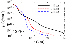
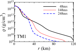
Figure 1: (Spherically-averaged) radial profiles of the rest-mass density at 48, 148, and 248 ms after core bounce. The left and right panel corresponds to SFHx and TM1, respectively.

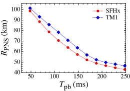
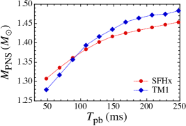
Figure 2: Time evolution of the PNS radius (left panel) and its gravitational mass (right panel) as a function of the postbounce time. The circles and diamonds corresponds to SFHx and TM1, respectively. The surface of the PNS is defined at a fiducial rest-mass density of $\rho_{s}=10^{10}$ g cm^-3.

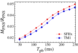
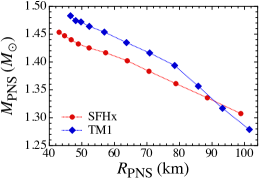
Figure 3: Left: Same as Fig. 2, but for the time evolution of the stellar compactness after bounce. Right: Sequences of the masses and radii of PNSs for SFHx and TM1. Note that the points at the left (smaller PNS radius) correspond to late postbounce phase, whereas the points at the right correspond to early phase (larger PNS radius).

The left panel of Fig. 3 shows the evolution of the “compactness” of the PNS that is defined by $M_{\rm PNS}/R_{\rm PNS}$ for SFHx (red line) and TM1 (blue line). As one would imagine, the compactness of the PNS is higher for SFHx compared to TM1 even after we consider the inaccuracy of $\sim 1\%$ in $M_{\rm PNS}$. The right panel of Fig. 3 depicts the time evolution of $M_{\rm PNS}$ as a function of $R_{\rm PNS}$. The PNS with the softer EOS (SFHx) evolves from larger to smaller PNS radius with bigger to smaller enclosed mass compared to the stiffer EOS (TM1). Depending on the stiffness of the EOSs, one can see that the evolution track in the $M_{\rm PNS}-R_{\rm PNS}$ plane differs significantly.

To extract the metric from the background models in a suitable form, we perform the following coordinate transformation. In the background models obtained by numerical relativity simulation (e.g., KKT2016 ), the line element is given as

$$ds^{2}=-\alpha^{2}dt^{2}+\gamma_{ij}(dx^{i}+\beta^{i}dt)(dx^{j}+\beta^{j}dt),$$ (1)

where $\alpha$, $\beta^{i}$, and $\gamma_{ij}$ are the lapse, shift vector, and three metric, respectively. If one assumes that the hydrodynamical background is static and spherically symmetric, the spacetime in the isotropic coordinates can also be written as

$$ds^{2}=-\frac{\left(1-\frac{M}{2\hat{r}}\right)^{2}}{\left(1+\frac{M}{2\hat{r}}\right)^{2}}dt^{2}+\left(1+\frac{M}{2\hat{r}}\right)^{4}(d\hat{r}^{2}+\hat{r}^{2}d\theta^{2}+\hat{r}^{2}\rm{sin}^{2}\theta d\phi^{2}),$$ (2)

where $\hat{r}$ and $M$ denote the isotropic radius $\hat{r}=\sqrt{x^{2}+y^{2}+z^{2}}$ and the enclosed gravitational mass, respectively. From Eqs. (1) and (2), one can easily check the validity of our static and spherically symmetric background assumption by comparing $\gamma_{\hat{r}\hat{r}}$ and $(1+M/2\hat{r})^{4}$ (see Appendix A for detail).

Next, we perform coordinate transformation from the isotropic, i.e. Eqs. (1) or (2), to the following spherically symmetric spacetime,

$$ds^{2}=-e^{2\Phi}dt^{2}+e^{2\Lambda}dr^{2}+r^{2}\left(d\theta^{2}+\sin^{2}\theta d\phi^{2}\right),$$ (3)

where $\Phi$ and $\Lambda$ are functions of only $r$. This metric is similar to the Schwarzschild metric and we apply the well-known conversion relation $r=\hat{r}(1+M/2\hat{r})^{2}$. In addition, $\Lambda$ is associated with the mass function $M$ in such a way that $e^{-2\Lambda}=1-2M/r$. With this metric form, the four-velocity of fluid element is given by $u^{\mu}=(e^{-\Phi},0,0,0)$.

III Perturbation equations for axial $w$-mode gravitational waves

On the PNS models mentioned in the previous section, we examine the oscillations and its spectra with the linear perturbation approach. In particular, when one focuses on axial type oscillations, the metric perturbation, $h_{\mu\nu}$, with the Regge-Wheeler gauge can be decomposed as

$$h_{\mu\nu}=\sum_{\ell=2}^{\infty}\sum_{m=-\ell}^{\ell}\left(\begin{array}[]{cccc}0&0&-h_{0,\ell m}{\sin^{-1}\theta}\partial_{\phi}&h_{0,\ell m}\sin\theta\,\partial_{\theta}\\ \ast&0&-h_{1,\ell m}{\sin^{-1}\theta}\partial_{\phi}&h_{1,\ell m}\sin\theta\,\partial_{\theta}\\ \ast&\ast&0&0\\ \ast&\ast&0&0\\ \end{array}\right)Y_{\ell m}\,,$$ (4)

where $Y_{\ell m}$ is the spherical harmonics with the angular indexes $\ell$ and $m$, noting that $h_{0,\ell m}$ and $h_{1,\ell m}$ are functions of $t$ and $r$ KS1999 . Additionally, the perturbation of the four-velocity is given by

$$\delta u^{\mu}=\sum_{\ell=2}^{\infty}\sum_{m=-\ell}^{\ell}\left(0,0,-\frac{\delta u_{\ell m}}{r^{2}\sin\theta}\partial_{\phi}Y_{\ell m},\frac{\delta u_{\ell m}}{r^{2}\sin\theta}\partial_{\theta}Y_{\ell m}\right),$$ (5)

while the perturbations of pressure and energy density should be zero for axial type oscillations.

The perturbation equation governing the axial type of GWs on the spherically symmetric background can be expressed as a single wave equation TC1967 ; CF1991 , such as

$$-\frac{\partial^{2}X_{\ell m}}{\partial t^{2}}+\frac{\partial^{2}X_{\ell m}}{\partial r_{*}^{2}}-e^{2\Phi}\left[\frac{\ell(\ell+1)}{r^{2}}-\frac{6m}{r^{3}}+4\pi(\varepsilon-p)\right]X_{\ell m}=0,$$ (6)

where $X_{\ell m}$ is related to the metric perturbation, $h_{1,\ell m}$, via $rX_{\ell m}=e^{\Phi-\Lambda}h_{1,\ell m}$, while $r_{*}$ is the tortoise coordinate defined as $r_{*}=r+2M\ln(r/2M-1)$. That is, $\partial_{r}=e^{\Lambda-\Phi}\partial_{r_{*}}$. The remaining variables, $h_{0,\ell m}$ and $\delta u_{\ell m}$, can be computed with $h_{1,\ell m}$ from the relations $\partial_{t}h_{0,\ell m}=e^{\Phi-\Lambda}X_{\ell m}+r\partial_{r_{*}}X_{\ell m}$ and $\delta u_{\ell m}=-e^{-\Phi}h_{0,\ell m}$. We remark that Eq. (6) outside the star reduces to the well-known Regge-Wheeler equation. Hereafter, we omit the index of $(\ell,m)$ for simplicity.

In fact, by solving this system one can obtain the specific oscillation spectra of GWs, i.e., the so-called $w$-modes wmode ; wmode1 . Replacing $X_{\ell m}$ in Eq. (6) with $X_{\ell m}(t,r)=X(r)\exp(i\omega t)$, one gets the perturbation equation with respect to the eigenvalue $\omega$,

$$X^{\prime\prime}+\left(\Phi^{\prime}-\Lambda^{\prime}\right)X^{\prime}+e^{2\Lambda}\left[\omega^{2}e^{-2\Phi}-\frac{\ell(\ell+1)}{r^{2}}+\frac{6m}{r^{3}}-4\pi(\varepsilon-p)\right]X=0.$$ (7)

By imposing appropriate boundary conditions, the problem to solve becomes the eigenvalue problem. The boundary conditions are the regularity condition at the stellar center and the outgoing wave condition at spatial infinity.

The eigenvalue $\omega$ becomes a complex number, because GWs carry out the oscillation energy, where the real and imaginary parts of $\omega$ correspond to the oscillation frequency ($f={\rm Re}(\omega)/2\pi$) and damping rate ($1/\tau={\rm Im}(\omega)$), respectively, where $\tau$ corresponds to the damping time of each mode. To determine such a complex frequency, we adopt the continuous fractional method proposed by Leaver Leaver .

IV Asteroseismology with $w$-modes

The spacetime modes ($w$-modes) have two families, i.e., $w_{\rm II}$ and “ordinary” $w$-modes wmode ; wmode1 . As shown in Appendix B, for cold NSs, a few $w_{\rm II}$-modes are excited, whose damping rate (${\rm Im}(\omega)$) is larger than its oscillation frequency (${\rm Re}(\omega)$). On the other hand, infinite number of $w$-modes can exist, which are referred to as $w_{1}$, $w_{2}$, $\cdots$, $w_{n}$-modes in order from the lowest oscillation frequency. So, in the similar way to cold NSs, we identify the spacetime modes with ${\rm Re}(\omega)$ larger than ${\rm Im}(\omega)$ as the “ordinary” $w$-modes for PNSs. Hereafter, the “ordinary” $w$-modes are called just as the $w$-modes.

In Fig. 4, we show the frequency and damping rate of the axial spacetime modes for the PNS models at the two postbounce times of $T_{\rm pb}=$ 108 ms (circles) and 248 ms (diamonds), where the left and right panels correspond to the results with SFHx and TM1 (EOS). In this figure, the open marks denote the $w_{\rm II}$-modes, while the solid marks denote the $w$-modes. Thus, the leftmost solid marks correspond to the $w_{1}$-mode (fundamental $w$-mode) for each PNS model. From this figure, one can observe that the damping rate of $w_{n}$-mode is almost constant independently of the index $n$, which is different behavior from the case of cold NSs as shown in Fig. 10. In fact, the damping rate of $w_{n}$-modes increase with the index $n$ for cold NSs. With respect to the $w_{1}$-mode (Fig. 5), we show the time evolution of the frequency ($f_{w_{1}}$) and damping time ($\tau_{w_{1}}$) as a function of postbounce time for SFHx and TM1, respectively. We remark that the damping time is the time with which the GW amplitude reduces by $1/e$. In the early phase of $w_{1}$-mode oscillations of PNSs, the frequency is only a few kHz, which is significantly smaller than that for cold NSs, while the damping time is around 0.1 ms, which is much larger than that for cold NSs. This is good news from the observational point of view. The direct detection of such a frequencies with the future (or even current) GW detectors might be possible, depending on the radiation energy of $w_{1}$-mode and the distance to a source object.

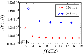
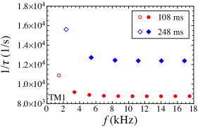
Figure 4: Frequency and damping rate of the axial spacetime modes for PNSs. The left and right panels correspond to the results for SFHx and TM1 EOSs, respectively, where the circles and diamonds are shown for the PNS models at 108 and 248 ms after core bounce. The open and solid marks correspond to the $w_{\rm II}$ and “ordinary” $w$-modes.

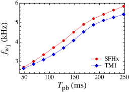
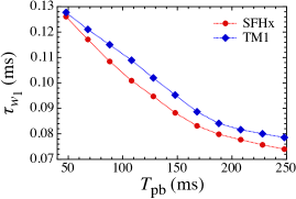
Figure 5: Evolutions of frequency $(f_{w_{1}})$ and damping time $(\tau_{w_{1}})$ for the $w_{1}$-mode. The circles and diamonds correspond to SFHx and TM1, respectively.

It is known that the frequency of $w_{1}$-mode for cold NSs can be characterized by the stellar compactness. That is, Andersson and Kokkotas have shown that for cold NSs the $w_{1}$-mode frequencies multiplied by the stellar radius are characterized by the stellar compactness independently of the EOS of neutron star matter AK1998 , such as

$$f_{w_{1}}^{\rm(NS)}\ {\rm(kHz)}\approx\left[20.92-9.14\left(\frac{M}{1.4M_{\odot}}\right)\left(\frac{R}{10\ {\rm km}}\right)^{-1}\right]\left(\frac{R}{10\ {\rm km}}\right)^{-1}.$$ (8)

This behavior comes from that the $w$-modes are oscillations of spacetime itself, which is almost independent from the matter oscillations. In the same way, the additional universal relation between the frequency of $f$-mode and stellar average density for cold NSs have been also derived AK1998 , such as

$$f_{f}^{\rm(NS)}\ {\rm(kHz)}\approx 0.78+1.635\left(\frac{M}{1.4M_{\odot}}\right)^{1/2}\left(\frac{R}{10\ {\rm km}}\right)^{-3/2}.$$ (9)

This means that, via the simultaneous observations of the frequencies of $f$- and $w_{1}$-modes, one can get two different information about the compact object, which enables us to constrain the mass and radius of source object. This is an original idea proposed by AK1998 to adopt the GW asteroseismology to the cold NSs. In this work, we revisit this in the context of the PNS, i.e., we will consider the possibility for obtaining the mass and radius of PNSs via the observations of the $f$- and $w_{1}$-modes GWs.

We find that the similar universal relation for $w_{1}$-mode can be held even for the PNSs. In Fig. 6, we show the $w_{1}$-mode frequencies multiplied by the radius as a function of the compactness, where the circles and diamonds correspond to the results for SFHx and TM1, respectively. As shown in Fig. 3, since the compactness increases with time, the left side in Fig. 6 corresponds to the early phase of PNSs. From this figure, we derive the fitting formula such as

$$f_{w_{1}}^{\rm(PNS)}\ {\rm(kHz)}\approx\left[27.99-12.02\left(\frac{M_{\rm PNS}}{1.4M_{\odot}}\right)\left(\frac{R_{\rm PNS}}{10\ {\rm km}}\right)^{-1}\right]\left(\frac{R_{\rm PNS}}{10\ {\rm km}}\right)^{-1}.$$ (10)

We remark that the $w_{1}$-mode frequencies for PNSs expected from this fitting formula are significantly different from those for cold NSs expected from Eq. (8), because the radius and mass of PNSs are different from those for cold NSs. We also remark that the scaling law for PNSs with using the mass and radius is the same as that for cold NSs, but the coefficients in the law are different. So, the coefficients in the scaling law would vary with time and eventually approach the values for cold NSs. This would suggest that long-term GW astroseismology and the GW detection could potentially bridge the gap of the two formulae evolving from a PNS phase into a cold NS phase.

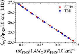
Figure 6: The $w_{1}$-mode frequencies multiplied by the normalized radius $f_{w_{1}}(R/10\ {\rm km})$ are shown as a function of normalized compactness $(M_{\rm PNS}/1.4M_{\odot})(R_{\rm PNS}/10\ {\rm km})^{-1}$, where the circles and diamonds denote the results for SFHx and TM1 EOSs, respectively. The dotted line is a fitting formula given by Eq. (10).

With respect to the $f$-mode on PNSs, we have derived the universal relation between the $f$-mode frequency and the average density of PNS independently of the progenitor models ST2016 . However, in order to consistently discuss the $f$-mode oscillations with the results of $w_{1}$-mode, we re-calculate by using the PNS models adopted in this paper with the same procedure as in ST2016 , i.e., with Cowling approximation neglecting the variation of entropy. Then, we get the time evolutions of $f$- and $p_{1}$-modes for SFHx and TM1 as shown in the left panel of Fig. 7. It should be noticed that even $p_{1}$-mode frequency might be possible to observe because the frequencies in the early phase of PNS are only a few hundred Hz. In the same way as shown in ST2016 , we also confirm that the frequencies of $f$-modes can be expressed as a linear function of the average density of PNS independently of the adopted EOS (see the right panel of Fig. 7), such as

$$f_{f}^{\rm(PNS)}\ {\rm(Hz)} \approx 14.48+4859\left(\frac{M_{\rm PNS}}{1.4M_{\odot}}\right)^{1/2}\left(\frac{R_{\rm PNS}}{10\ {\rm km}}\right)^{-3/2},$$ (11)

$$f_{p_{1}}^{\rm(PNS)}\ {\rm(Hz)} \approx 43.29+8602\left(\frac{M_{\rm PNS}}{1.4M_{\odot}}\right)^{1/2}\left(\frac{R_{\rm PNS}}{10\ {\rm km}}\right)^{-3/2},$$ (12)

where the coefficients in the linear fits are modified a little from the previous one because the surface density of the PNS models adopted in this paper is different from that in ST2016 . In practice, these linear fits are also shown in the middle and right panels of Fig. 7 with solid lines. We remark that the frequencies of the $f$- and $p_{1}$-modes are the same dependence on the properties of PNSs, i.e., one can get only the information about the average density of PNS even if one will simultaneously detect the $f$- and $p_{1}$-modes.

Consequently, one can obtain the information of two different properties, which are combinations of $M_{\rm PNS}$ and $R_{\rm PNS}$, via Eqs. (10) and (11) (or via Eqs. (10) and (12)), if one would simultaneously detect the $f$- and $w_{1}$-modes (or the $p_{1}$- and $w_{1}$-modes) in GWs from PNSs, which enables us to know the values of $M_{\rm PNS}$ and $R_{\rm PNS}$. Furthermore, unlike the GW asteroseismology for cold NSs, for PNSs one might get the sequence in $M_{\rm PNS}-R_{\rm PNS}$ plain as shown in Fig. 3 with the time evolution of the GW spectra from the PNS produced by just one supernova explosion, because $M_{\rm PNS}$ and $R_{\rm PNS}$ changes with time. Namely, in principle one would find the EOS via the detection of the GWs from just one supernova explosion.

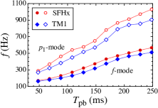
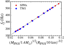
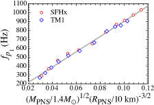
Figure 7: Evolutions of $f$- and $p_{1}$-modes in GWs from PNSs after core bounce are shown in the left panes. The solid and open marks correspond to the $f$- and $p_{1}$-modes, while the circles and diamonds are respectively the results for SFHx and TM1. The middle and right panels shows respectively the frequencies of the $f$- and $p_{1}$-modes as a function of average density of PNSs. The solid line denotes the linear fitting given by Eqs. (11) and (12).

Finally, we discuss the detectability of GWs from PNSs. In Refs. AK1996 ; AK1998 , the effective amplitude of $f$- and $w_{1}$-modes in GWs radiating from cold NSs are estimated, where the background stellar model should be static at least during the damping time. Since the damping time of $w_{1}$-mode from PNSs is typically $\tau_{w_{1}}\sim 0.1$ ms as shown in Fig. 5, which is shorter than the typical timescale of change of PNS properties, one might possible to adopt the estimation of effective amplitude for $w_{1}$-mode derived in AK1996 ; AK1998 even for PNSs. On the other hand, if one estimates the damping time of $f$-mode for PNSs in the same way as for cold NSs, such as $\tau_{f}\sim R_{\rm PNS}^{4}/M_{\rm PNS}^{3}$ AK1998 , $\tau_{f}$ becomes $\sim 1-50$ second, which is much larger than the typical timescale of change of PNS properties. Thus, it must be inappropriate to adopt the estimation of effective amplitude for $f$-mode derived in AK1996 ; AK1998 in the case of PNSs. Thus, here we only consider the detectability of $w_{1}$-mode in gravitational waves. Even so, we may deduce that the upper limit of the effective amplitude of the $f$-mode in gravitational waves from PNSs would be around $h\sim 10^{-21}$, assuming that the $f$-mode oscillations can be also captured as well as the other excited modes in the previous numerical simulations of core-collapse supernovae CDAF2013 ; KKT2016 ; Andresen16 .

For PNSs, we choose that the energy of $w_{1}$-mode in the gravitational waves, $E_{w_{1}}$, for each time step, and estimate the effective amplitude of such gravitational waves with the same formula as in AK1996 ; AK1998 . Thus, the effective amplitude is given by

$$h_{\rm eff}^{(w_{1})}\sim 7.7\times 10^{-23}\left(\frac{E_{w_{1}}}{10^{-10}\ M_{\odot}}\right)^{1/2}\left(\frac{4\ {\rm kHz}}{f_{w_{1}}}\right)^{1/2}\left(\frac{10\ {\rm kpc}}{D}\right),$$ (13)

where $D$ denotes the distance between the source and the Earth. We remark that the effective amplitude depends on the frequencies of $w_{1}$-mode, which change with time. Assuming the total radiation energy with $w_{1}$-mode in the gravitational waves from PNS ($E_{\rm T}^{(w_{1})}$), the energy for each time step ($E_{w_{1}}$) can be estimated as $E_{\rm T}^{(w_{1})}\approx E_{w_{1}}T_{w_{1}}/\tau_{w_{1}}$, where $T_{w_{1}}$ denotes the duration time of $w_{1}$-mode. In this paper, we simply assume that $T_{w_{1}}=250$ ms and $\tau_{w_{1}}=0.1$ ms. Since the total energy of $w_{1}$-mode in gravitational waves is also unknown, we consider five cases, i.e., $10^{-4}M_{\odot}$, $10^{-5}M_{\odot}$, $10^{-6}M_{\odot}$, $10^{-7}M_{\odot}$, and $10^{-8}M_{\odot}$, as the values of $E_{\rm T}^{(w_{1})}$. Then, the expected effective amplitude of $w_{1}$-mode in gravitational waves radiated from PNSs with SFHx EOS is shown in Fig. 8 together with the sensitivity curves of KAGRA, advanced LIGO, Einstein Telescope, and Cosmic Explorer aso13 ; CE ; CE2 . In this figure, the circles, squares, diamonds, triangles, and upside-down triangles denote for the cases with $E_{\rm T}^{(w_{1})}=10^{-4}M_{\odot}$, $10^{-5}M_{\odot}$, $10^{-6}M_{\odot}$, $10^{-7}M_{\odot}$, and $10^{-8}M_{\odot}$, respectively. The leftmost marks of the effective amplitude for each mode correspond to the PNS model at 48 ms after core bounce, and the effective amplitude decreases with time. From this figure, the radiation energy of $E_{\rm T}^{(w_{1})}=10^{-5}M_{\odot}$ seems to be marginal for the advanced LIGO.

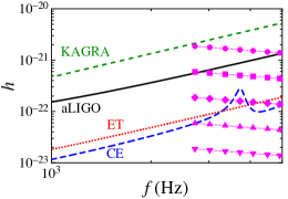
Figure 8: The effective amplitude of $w_{1}$-modes in gravitational waves radiated from the PNSs with SFHx EOS are shown together with the sensitivity curves of KAGRA, advanced LIGO (aLIGO), Einstein Telescope (ET), and Cosmic Explorer (CE). The circles, squares, diamonds, triangles, and upside-down triangles correspond to the results with $E_{\rm T}^{(w_{1})}=10^{-4}M_{\odot}$, $10^{-5}M_{\odot}$, $10^{-6}M_{\odot}$, $10^{-7}M_{\odot}$, and $10^{-8}M_{\odot}$, respectively.

V Conclusion

The GWs radiated from supernova explosions are one of the most promising sources. In this paper, we considered the GWs emitted from a PNS in the postbounce phase of core-collapse supernovae. In particular, we focused on the spacetime mode, the so-called $w$-mode. Regarding the background model, we used results from most recent 3D-GR models. Then, we calculated the complex frequencies on such PNS models, assuming that the PNS model on each time step is static spherically symmetry. The real and imaginary parts of complex frequency correspond to the oscillation frequency and the damping rate.

We have found that the damping rate of $w_{n}$-modes for PNSs is almost independent from the index $n$, although that for cold NSs increases with $n$. Moreover, in the similar way to the case for cold NSs, we found that the $w_{1}$-mode frequency multiplied by the PNS radius can be expressed as a linear function of the compactness of PNSs independently of EOSs. The $w_{1}$-mode frequency of PNSs just after the core-bounce is typically around a few kHz, which might be better from the observational point of view. Using such a universal relation for $w_{1}$-mode frequency together with another universal relation for $f$-mode, where the frequency can be expressed as a linear function of the square root of the average density of PNSs independently of the progenitor models, one can get two different properties constructed with the mass and radius of the PNS, if one would detect simultaneously the both modes. Therefore, one would determine the mass and radius of PNSs in principle on each time step, which would enable us to study the finite-temperature EOS that predominantly determines the PNS evolution.

Appendix A Validity of the static and spherically symmetric assumption for our 3D models

From Eqs. (1) and (2), one can check the validity of our static and spherically symmetric assumption by comparing $\gamma_{\hat{r}\hat{r}}$ and $(1+M/2\hat{r})^{4}$. In Fig. 9, we plot the gravitational mass $M$ (cross) and the effective mass $2\hat{r}({\gamma_{\hat{r}\hat{r}}}^{1/4}-1)$ (solid line) at representative post bounce times $T_{\rm pb}=48$, 148, and 248 ms. The inner mini panel is a magnified view where the solid lines and crosses deviate the most. For $M$, we simply adopt the following ADM mass

$$M = \int dx^{3}\left[\rho_{\rm H}\psi^{5}+\frac{\psi^{5}}{16\pi}\Bigl{(}\tilde{A}_{ij}\tilde{A}^{ij}-\frac{2}{3}K^{2}-{\gamma}^{ij}\tilde{R}_{ij}\Bigr{)}\right],$$ (14)

where $\rho_{\rm H}=\rho hW^{2}-P$, with $\rho$, $h$, $W$, and $P$ being the rest mass density, enthalpy, Lorentz factor, and pressure, respectively, and $\psi$, $\tilde{A}_{ij}$, $K$, and $\tilde{R}_{ij}$ are the conformal factor, tracefree part of the extrinsic curvature, trace of the extrinsic curvature, and the Ricci tensor with respect to $\tilde{\gamma}_{ij}={\gamma}_{ij}\psi^{-4}$, respectively. Because of the highly convective motion within the shock radius $\hat{r}\lesssim 100$ km, the effective gravitational mass calculated from $\gamma_{\hat{r}\hat{r}}$ does not match with $M$. The maximum deviation however is a few percent and we consider that it is sufficient to describe the background metric with $M$ instead of using simply $\gamma_{\hat{r}\hat{r}}$, since the effective gravitational mass at $\hat{r}\sim 30-$50 km (solid line in the mini panel) has a negative gradient. In any way, we confirm that the resultant $w$-mode frequencies and damping rates with the actual mass we adopted in text are almost the same as those with the effective mass determined from $\gamma_{\hat{r}\hat{r}}$. For example, the difference in the $w_{1}$-mode frequency at 248 ms between the results with actual and effective masses is only $0.23\%$ for SFHx and $0.14\%$ for TM1, while the difference in the $w_{1}$-mode damping rate at 248 ms is only $0.98\%$ for SFHx and $0.91\%$ for TM1.

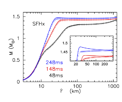
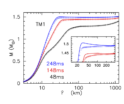
Figure 9: The effective (solid) and actual (cross) gravitational mass as a function of the isotropic radius $\hat{r}$ at 48, 148, and 248 msec after core bounce. The left and right panels correspond to the results with SFHx and TM1 EOSs, respectively.

Appendix B $w$-mode for cold neutron stars

For reference, in Fig. 10 we show the complex frequencies of $w$-mode oscillations from a cold neutron star with $1.5M_{\odot}$ constructed with the Shen EOS Shen . In this figure, the open circle corresponds to the $w_{\rm II}$-mode, while the solid circles are the $w$-modes. The $w$-modes are called as $w_{1}$, $w_{2}$, $\cdots$, $w_{n}$-modes from the lower frequencies. For the case of cold NSs, it is known that the damping rate of $w$-mode increases as the mode becomes higher-order oscillations wmode ; wmode1 , as shown in this figure.

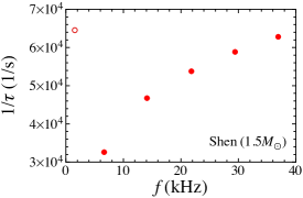
Figure 10: Typical frequency and damping rate of spacetime modes for a cold neutron star. This is a result for the neutron star with $1.5M_{\odot}$, which is constructed with the Shen EOS. The open and solid circles correspond to the $w_{\rm II}$ and “ordinary” $w$-modes, respectively.

References

- (1) B. P. Abbott et al. (LIGO Scientific Collaboration and Virgo Collaboration), Phys. Rev. Lett. 116, 061102 (2016).
- (2) B. P. Abbott et al. (LIGO Scientific Collaboration and Virgo Collaboration), Phys. Rev. Lett. 116, 241103 (2016).
- (3) S. Hild, A. Freise, M, Mantovani, M., et al. Classical and Quantum Gravity, 26, 025005 (2009).
- (4) Y. Aso, Y. Michimura, K. Somiya, K., et al. Phys. Rev. D, 88, 043007 (2013).
- (5) M. Punturo, H. Lück, & M. Beker, Advanced Interferometers and the Search for Gravitational Waves, 404, 333, (2014).
- (6) B. P. Abbott et al. (LIGO Scientific Collaboration and Virgo Collaboration), Class. Quantum Grav. 34, 044001 (2017).
- (7) B. S. Sathyaprakash and B. F. Schutz, Living Reviews in Relativity, 12, 2, (2009)
- (8) N. Andersson, Classical and Quantum Gravity, 20, R105, (2003)
- (9) K. Kotake, Comptes Rendus Physique 14, 318 (2013).
- (10) B. Müller, H. -T. Janka, and A. Marek, Astrophys. J. 766, 43 (2013).
- (11) P. Cerdá-Durán, N. DeBrye, M. A. Aloy, J. A. Font, and M. Obergaulinger, Astrophys. J. Lett. 779, L18 (2013).
- (12) T. Kuroda, K. Kotake, and T. Takiwaki, Astrophys. J. Lett. 829, L14 (2016).
- (13) C. D. Ott, E. Abdikamalov, P. Mösta, R. Haas, S. Drasco, E. P. O’Connor, C. Reisswig, C. A. Meakin, and E. Schnetter, Astrophys. J. 768, 115 (2013).
- (14) H. Andresen, B. Müller, E. Müller, and H.-T. Janka, Mon. Not. R. Astron. Soc. 468, 2032, (2017).
- (15) J. W. Murphy, C. D. Ott, and A. Burrows, Astrophys. J. 707, 1173 (2009).
- (16) K. N. Yakunin, A. Mezzacappa, P. Marronetti, S. Yoshida, S. W. Bruenn, W. R. Hix, E. J. Lentz, O. E. B. Messer, J. A. Harris, E. Endeve, J. M. Blondin, and E. J. Lingerfelt, Phys. Rev. D 92, 084040 (2015).
- (17) J. M. Blondin, A. Mezzacappa, and C. DeMarino, Astrophys. J. 584, 971 (2003).
- (18) T. Foglizzo, L. Scheck, and H.-T. Janka, Astrophys. J. 652, 1436 (2006).
- (19) E. O’Connor and C. D. Ott, Astrophys. J. 730, 70, (2011).
- (20) F. Hanke, B, Müller, A. Wongwathanarat, A. Marek, and H.-T. Janka, Astrophys. J. 770, 66 (2013).
- (21) K. Nakamura, T. Takiwaki, T. Kuroda, T, and K. Kotake, Publ. Astron. Soc. Japan, 67, 107, (2015).
- (22) K. D. Kokkotas and B. G. Schmidt, Living Rev. Relativ. 2, 2 1999.
- (23) A. W. Steiner and A. L. Watts, Phys. Rev. Lett. 103, 181101 (2009).
- (24) M. Gearheart, W. G. Newton, J. Hooker, and B. -A. Li, Mon. Not. R. Astron. Soc. 418, 2343 (2011).
- (25) H. Sotani, K. Nakazato, K. Iida, and K. Oyamatsu, Phys. Rev. Lett. 108, 201101 (2012).
- (26) H. Sotani, K. Nakazato, K. Iida, and K. Oyamatsu, Mon. Not. R. Astron. Soc. 428, L21 (2013).
- (27) H. Sotani, K. Nakazato, K. Iida, and K. Oyamatsu, Mon. Not. R. Astron. Soc. 434, 2060 (2013).
- (28) H. Sotani, K. Iida, and K. Oyamatsu, New Astron. 43, 80 (2016).
- (29) H. Sotani, K. Iida, and K. Oyamatsu, Mon. Not. R. Astron. Soc. 464, 3101 (2017).
- (30) N. Andersson and K. D. Kokkotas, Phys. Rev. Lett. 77, 4134 (1996).
- (31) N. Andersson and K. D. Kokkotas, Mon. Not. R. Astron. Soc. 299, 1059 (1998).
- (32) H. Sotani, K. Tominaga, and K. I. Maeda, Phys. Rev. D 65, 024010 (2001).
- (33) H. Sotani and T. Harada, Phys. Rev. D 68, 024019 (2003); H. Sotani, K. Kohri, and T. Harada, ibid. 69, 084008 (2004).
- (34) H. Sotani, N. Yasutake, T. Maruyama, and T. Tatsumi, Phys. Rev. D 83 024014 (2011).
- (35) A. Passamonti and N. Andersson, Mon. Not. R. Astron. Soc. 419, 638 (2012).
- (36) D. D. Doneva, E. Gaertig, K. D. Kokkotas, and C. Krüger, Phys. Rev. D 88 044052 (2013).
- (37) V. Ferrari, G. Miniutti, and J. A. Pons, Mon. Not. R. Astron. Soc. 342, 629 (2003).
- (38) J. Fuller, H. Klion, E. Abdikamalov, and C. D. Ott, Mon. Not. R. Astron. Soc. 450, 414 (2015).
- (39) H. Sotani and T. Takiwaki, Phys. Rev. D 94, 044043 (2016).
- (40) G. Camelio, A. Lovato, L. Gualtieri, O. Benhar, J. A. Pons, and V. Ferrari, arXiv:1704.01923.
- (41) H.-T. Janka, T. Melson, and A. Summa, Annual Review of Nuclear and Particle Science, 66, 341, (2016).
- (42) B. Müller, PASA, 33, e048, (2016).
- (43) K. Kotake, K. Sumiyoshi, S. Yamada. et al., Progress of Theoretical and Experimental Physics, 01A301, (2012).
- (44) K. D. Kokkotas and B. F. Schutz, Mon. Not. R. Astron. Soc. 255, 119 (1992).
- (45) M. Leins, H. -P. Nollert, and M. H. Soffel, Phys. Rev. D 48, 3467 (1993).
- (46) N. Andersson, Y. Kojima, and K. D. Kokkotas, Astrophys. J. 462, 855 (1996).
- (47) T. Kuroda, K. Kotake, and T. Takiwaki, Astrophys. 755, 11, (2012).
- (48) S. E. Woosley and T. A. Weaver, ApJS, 101, 181, (1995).
- (49) A. W. Steiner, M. Hempel, and T. Fischer, Astrophys. J. 774, 17 (2013).
- (50) M. Hempel and J. Schaffner-Bielich, Nucl. Phys. A 837, 210 (2010).
- (51) T. Fischer, M. Hempel, I. Sagert, Y. Suwa, and J. Schaffner-Bielich, Euro. Phys. J. A 50, 46 (2014).
- (52) A. W. Steiner, J. M. Lattimer, and E. F. Brown, Astrophys. J. 722, 33 (2010).
- (53) M. B. Tsang, et al., Phys. Rev. C 86, 015803 (2012).
- (54) P. B. Demorest, T. Pennucci, S. M. Ransom, M. S. E. Roberts, and J. W. T. Hessels, Nature 467, 1081 (2010).
- (55) Antoniadis, J., Freire, P. C. C., Wex, N., et al. 2013, Science, 340, 448
- (56) T. Takiwaki, K. Kotake, and Y. Suwa, Astrophys. J, 786, 83, (2014).
- (57) K. S. Thorne and A. Campolattaro, Astrophys. J. 149, 591 (1967).
- (58) S. Chandrasekhar and V. Ferrari, Proc. R. Soc. A 432, 247 (1991).
- (59) E. W. Leaver, Proc. R. Soc. London A402, 285 (1985).
- (60) T. Regimbau, M. Evans, N. Christensen, E. Katsavounidis, B. Sathyaprakash, S. Vitale, Phys. Rev. Lett. 118, 151105 (2017).
- (61) H. Shen, H. Toki, K. Oyamatsu, and K. Sumiyoshi, Nucl. Phys. A 637, 435 (1998).