One-dimensional Bose gas dynamics: breather relaxation

Abstract

One-dimensional Bose gases are a useful testing-ground for quantum dynamics in many-body theory. They allow experimental tests of many-body theory predictions in an exponentially complex quantum system. Here we calculate the dynamics of a higher-order soliton in the mesoscopic case of $N=10^{3}-10^{4}$ particles, giving predictions for quantum soliton breather relaxation. These quantum predictions use a truncated Wigner approximation, which is a $1/N$ expansion, in a regime where other exactly known predictions are recovered to high accuracy. Such dynamical calculations are testable in forthcoming BEC experiments.

Techniques for observing near lossless quantum dynamics have led to quantitative tests of quantum field dynamics in photonic systems Rosenbluh and Shelby (1991); Drummond et al. (1993); Heersink et al. (2005); Corney et al. (2006). Improvements in ultra-cold quantum gas experiments mean that these experiments can now also compare first principles calculations of many-body quantum dynamics with observations Egorov et al. (2011). The 1D Bose gas, with its well-understood conservation laws Thacker (1981) and exact solutions Lieb and Liniger (1963); McGuire (1964) is an excellent testing ground for these ideas. Second-order correlations in thermal equilibrium with repulsive interactions have been predicted Gangardt and Shlyapnikov (2003); Kheruntsyan et al. (2003, 2005); Yurovsky et al. (2008) and verified experimentally Laburthe Tolra et al. (2004); Kinoshita et al. (2005). In these systems, there is evidence of steady-states that do not have a Gibbs structure Langen et al. (2015); Rigol et al. (2007). Attractive matter-wave solitons have also been experimentally observed Khaykovich et al. (2002); Strecker et al. (2002); Medley et al. (2014); McDonald et al. (2014); Nguyen et al. (2014, 2017).

Here we show that the dynamical stability of higher-order matter-wave solitons prepared by quenching is experimentally testable. Fragmentation and damping of breathing oscillations Weiss and Carr (2016); Yurovsky et al. (2017) are predicted to persist even up to a mean particle number of $N=1000$. These calculations use the truncated Wigner approximation, which is a $1/N$ expansion Graham (1973); Drummond and Hardman (1993); Steel et al. (1998). Known conserved quantities are replicated with high accuracy. This is a regime accessible to current BEC experiments Yurovsky et al. (2017); Everitt et al. (2017); Nguyen et al. (2017). We show that direct experimental tests of predictions for soliton fragmentation and center-of-mass dynamics are possible in an exponentially complex regime where exact calculation is extremely difficult.

Fragmentation causes a decay in oscillation that is predicted to happen gradually, without the abrupt changes after a short evolution time found by variational methods Streltsov et al. (2008). Such methods are known to disagree with exact COM spreading results Cosme et al. (2016), which means that they violate Galilean invariance Tao (2006). We show that this is because the number of dissociation channels is much larger than the number of variational modes used in such calculations. The oscillation decay found here is slower than predicted at very small particle number Weiss and Carr (2016), and also less pronounced than the predicted fragmentation at small $N$ obtained from exact analysis Yurovsky et al. (2017). However, this difference is qualitatively consistent with the scaling we find with $N$: where fragmentation and breather relaxation are reduced as $N$ increases.

Here we investigate the dynamics of a higher-order soliton or breather. In this case, even more dramatic effects can occur due to quantum fragmentation. Due to the enormous state-space, direct calculation with exact eigenstates is not practical in the regime of experimental interest, with $1000$ particles or more.

This has been the topic of several publications. The first Streltsov et al. (2008) used a multi-configurational time-dependent Hartree method for bosons (MCTDHB) approach with $N=1000$ and two spatial modes, predicting a sudden break-up into a pair of equal size fragments. This calculation was recently shown to be not fully converged, violating known quantum center-of-mass (COM) expansion physics Cosme et al. (2016). Our results confirm this earlier analysis. The predictions obtained here are completely different, with no evidence of a sudden breakup after a fixed evolution time.

Other approaches have used either exact methods Yurovsky et al. (2017), or matrix product states Weiss and Carr (2016). These were limited in number to $N<20$. Here we investigate larger particle numbers, i.e., $N=10^{3}-10^{4}$, and large numbers of independent modes, of order $10^{5}$. This is an experimentally realistic regime. Our calculations preserve all local conservation laws and (nearly) exact COM dynamics, giving results that are both quantitatively and qualitatively different to earlier variational studies.

In one dimensional optical or atomic waveguides, a similar Hamiltonian applies to either massive atomic Bose-Einstein condensate (BEC) experiments or to photonic experiments, where dispersion gives rise to an effective mass. If the bosons are confined to a single transverse mode, one obtains an 1D Bose gas theory, valid for low energies:

$$\hat{H}_{\mathrm{1D}}= \frac{\hbar^{2}}{2m}\int\hat{\Psi}_{\mathrm{1D}}^{\dagger}H_{1}\hat{\Psi}_{\mathrm{1D}}dr_{3}$$

$$+\frac{g_{\mathrm{1D}}}{2}\int\left(\hat{\Psi}_{\mathrm{1D}}^{\dagger}\right)^{2}\hat{\Psi}_{\mathrm{1D}}^{2}dr_{3}\,.$$ (1)

Here, $\bm{r}$ is the spatial coordinate, with a one-dimensional confinement so the dynamics occur in the $r_{3}$ direction. The mass is $m$, and for an atomic Bose gas in a parabolic trap one has:

$$H_{1} =-\hbar^{2}\partial_{3}^{2}/2m+m\omega_{3}^{2}r_{3}^{2}/2$$

$$g_{\mathrm{1D}} =2\hbar\omega_{\perp}a\,,$$ (2)

where $a$ is the three-dimensional S-wave scattering length, and the effective transverse trapping frequency of: $\omega_{\perp}=\sqrt{\omega_{1}\omega_{2}}$. If the system is photonic or polaritonic, as in a fibre optical experiment Drummond and Carter (1987); Drummond et al. (1993); Drummond and Hardman (1993), the relevant parameters come from the dispersion and optical nonlinearity properties of the fiber.

This can be transformed to dimensionless form by choosing a length scale $r_{0}$ and time scale $t_{0}$ such that $r_{0}^{2}=\hbar t_{0}/2m$. Distance is scaled to so that $z=r_{3}/r_{0}$, and time is scaled to give a dimensionless time $\tau=t/t_{0}$. The resulting Hamiltonian, in the form introduced by Lieb and Liniger Lieb and Liniger (1963), with a dimensionless wave-function $\hat{\psi}=\sqrt{r_{0}}\hat{\Psi}_{\mathrm{1D}}$, is:

$$\hat{H}=\int dz\left[\hat{\psi}_{,z}^{\dagger}(z)\hat{\psi}_{,z}(z)+C\left(\hat{\psi}^{\dagger}(z)\right)^{2}\hat{\psi}^{2}(z)\right].$$ (3)

We use a subscript to indicate a derivative, so that:

$$\hat{\psi}_{,z}(z)\equiv\partial_{z}\hat{\psi}(z)\equiv\frac{\partial}{\partial z}\hat{\psi}(z)\,.$$ (4)

The following relationships exist between the physical and dimensionless units in the case of a trapped Bose-Einstein condensate Olshanii (1998); Kheruntsyan et al. (2005): $\hat{H}=\hat{H}_{1}/E_{0}$, $E_{0}=\hbar/t_{0}=\hbar^{2}/2mr_{0}^{2}$ and $C=mg_{\mathrm{1D}}r_{0}/\hbar^{2}=2m\omega_{\perp}r_{0}a/\hbar$. A convenient procedure for solitons is to simply define $r_{0}$ as the characteristic initial dimension, so that $C$ is of the order of the inverse particle number $N$.

The corresponding dynamical equation is known as the one-dimensional quantum nonlinear Schrodinger equation. It also describes quantum photonic propagation in one-dimensional optical fibers Carter et al. (1987), under similar conditions of tight transverse confinement. Thus, an almost identical picture holds for 1D photonic systems Carter et al. (1987); Drummond and Carter (1987), except for additional Raman-Brillouin coupling to phonons, owing to the use of dielectric waveguides Gordon (1986); Carter and Drummond (1991). This earlier work used phase-space techniques that originate in the work of Wigner Wigner (1932) and Glauber Glauber (1963). Such predictions have been experimentally verified Rosenbluh and Shelby (1991); Drummond and Carter (1987); Corney et al. (2008). In both the photonic and atomic experiments, there are additional dissipative couplings due to linear and nonlinear losses and phase noise, leading to additional corrections. For simplicity, dissipation is ignored here, which limits the applicable interaction time.

The initial quantum states of experimental photonic pulses or BECs typically has a shot-to-shot randomness in the state preparation that results in experimental number fluctuations. It is common to have at least a Poissonian number variance Chuu et al. (2005) when the atom numbers are larger than $10^{3}$. Accordingly, we assume Poissonian number fluctuations in the calculations given here, in order to represent typical initial quantum density matrices. The Wigner distribution $W\left[\psi\right]$ over Wigner fields $\psi$ exists for any quantum state Wigner (1932); Hillery et al. (1984). It is not always positive definite. The usual operator time-evolution equation

$$\frac{d\hat{\psi}}{dt}=-i\left[\hat{H},\hat{\psi}\right],$$ (5)

where the Hamiltonian $\hat{H}$ is defined by Eq. (3), can be transformed Moyal (1949) into a differential equation for $W\left[\psi\right]$, typically with third or higher order derivatives. After truncation of third order derivatives Graham (1973), which are the highest order terms in a $1/N$ expansion for $N$ particles, one obtains a second order Fokker-Plank equation for $W\left[\psi\right]$. This is an approximate functional differential equation for a probability distribution over Wigner fields.

When the evolution is unitary, this results in a partial differential equation for phase-space variables using well-known procedures Steel et al. (1998); Opanchuk and Drummond (2013); Drummond and Hardman (1993). The resulting equation for the Wigner field $\psi$, is:

$$\frac{d\psi}{dt}=i\nabla^{2}\psi-2iC\psi\left(|\psi^{2}|-1/\Delta z\right),$$ (6)

where $\Delta z$ is the lattice spacing or inverse momentum cutoff. Quantum noise is present in the initial conditions. We start from a state with Poissonian number distribution, which is equivalent to a coherent state:

$$\hat{\rho}\left(t=0\right)=|\alpha\left(z\right)\rangle\langle\alpha\left(z\right)|,$$ (7)

where $|\alpha\left(z\right)|^{2}=n\left(z\right)$. In the Wigner representation this is exactly represented by an ensemble of fields $\psi\left(z\right)$ with initial quantum noise $\eta_{k}$, with

$$\psi\left(z\right)=\sqrt{n\left(z\right)}+\frac{1}{\sqrt{2}}\sum_{k}\frac{1}{\sqrt{L}}\eta_{k}e^{ikz}.$$ (8)

Here $\eta_{k}$ are complex random numbers correlated as $\langle\eta_{k}\eta_{k^{\prime}}^{*}\rangle=\delta_{kk^{\prime}}$, $\langle\eta_{k}\eta_{k^{\prime}}\rangle=0$. The functional integration over the Wigner distribution is performed by generating multiple random initial states and using them to seed independent integrations of the PDE. This results in a large number, $N_{\mathrm{s}}$, of independent field modes — each evolving in time with equal probability.

The Wigner phase-space method generates a direct representation of symmetrically ordered quantum observables. To obtain the usual normally-ordered quantum observables, one must transform the results of a Wigner calculation from a symmetrically ordered to a normally ordered form. This also removes the divergence of symmetrically-ordered observables at large momentum cutoff. The expectation values of symmetrically ordered operator expressions can be obtained by integrating this equation over multiple independent trajectories to produce a set of values $\psi^{(j)}$ and averaging over a corresponding function of these values.

There is an approximate equality between symmetrically ordered quantum averages and Wigner averages, where the $N$-dependent truncation error depends on the evaluated operator Kinsler et al. (1993); Kinsler (1996):

$$\left\langle\left\{\hat{O}\left(\hat{\psi},\hat{\psi}^{\dagger}\right)\right\}\right\rangle\approx\left\langle\left\{\hat{O}\right\}\right\rangle_{W}=\langle O\rangle_{W}.$$ (9)

We consider a quantum dynamical experiment where an initial state is prepared and then evolved in time. The initial state is a Poissonian mixture of uncorrelated particles with mean value $N=10^{3}-10^{4}$ in a localized spatial mode. The equivalent coherent state has the classical soliton shape that occurs with some small initial coupling of $C_{i}=-2/N$, with $r_{0}$ as the characteristic initial size, so that in dimensionless units, $\alpha(z)=\sqrt{N/2}\,\mathrm{sech}(z)$.

This corresponds to an ultra-cold atomic Bose gas experiment, with a BEC initially trapped in a localized state with no interactions. At time $t=0$, the interaction Hamiltonian is turned on to a larger value of $C_{f}=-8/N$, allowing particles to interact and forming a breather, a higher-order oscillating soliton. The resulting density profile, $\left\langle\hat{n}\left(z\right)\right\rangle=\left\langle\hat{\psi}^{\dagger}(z)\hat{\psi}(z)\right\rangle$, is shown in Fig. 1 for $N=1000$ and in Fig. 2 for $N=10000$. The result of the initial condition is that a high-order soliton or breather is formed Wai et al. (1986), with a characteristic period of $\tau_{b}=\pi/4$. Our numerical results show characteristic breathing oscillations such that the mean breather amplitude decays with time.

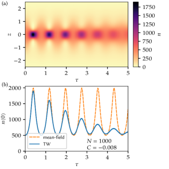
Figure 1: Density near the centre of the simulation area (a) and at $z=0$ (b) over time. Simulation with $N=10^{3}$, $C=-8\times 10^{-3}$, $M=512$, $L=20$, $10^{5}$ trajectories, $10^{5}$ time steps. The area between the simulation curves (solid blue lines) denotes the estimated sampling error. The result of the mean-field simulation (dashed orange lines) are shown for comparison. The time-step errors are smaller than the line thickness and are not shown on the graph.

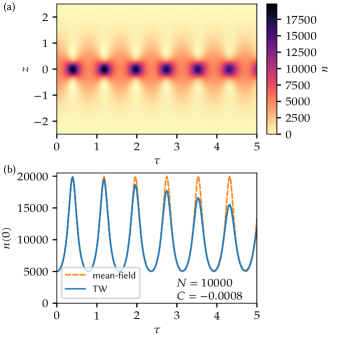
Figure 2: Density near the centre of the simulation area (a) and at $z=0$ (b) over time. Simulation with $N=10^{4}$, $C=-8\times 10^{-4}$, other properties as in Fig. 1.

This simulation is similar to related experimental proposals of first creating a fundamental soliton at weak coupling, then suddenly increasing the coupling strength. The coupling change would be caused by either a pulse entering a fiber in a photonic experiment, or else a change in a tunable Feshbach resonance in an atomic system. A number of different theoretical methods Streltsov et al. (2008); Weiss and Carr (2016); Yurovsky et al. (2017) have been used to analyze this type of proposed experiment, making it of topical interest. The present protocol employs a localized non-interacting BEC as the initial state, following earlier proposals Streltsov et al. (2008); Cosme et al. (2016). The timescales and numbers used are within the general parameter range achievable with current ⁷Li Nguyen et al. (2017) and ⁸⁵Rb Everitt et al. (2017) ultra-cold atomic physics experiments.

The simulation is sensitive to the selected spatial and momentum grids. The spatial grid must be symmetrical around 0 and have a point at $z=0$, or else the decay happens on a faster scale, since there is insufficient lattice resolution for spatial convergence. The momentum grid should ideally be symmetrical around 0, which can be achieved by using a pair of position- and momentum-dependent coefficients applied before and after the Fourier transform. If this condition is not satisfied, the unbalanced high-momentum components of the noise lead to numerical errors. A finite lattice was used with periodic boundary conditions at $z=\pm L/2$. Results were obtained using a public domain stochastic partial differential equation code Kiesewetter et al. (2016) with a fourth-order Runge-Kutta interaction picture algorithm Caradoc-Davies (2000), then cross-checked with a larger number of samples using an open source graphical processor unit (GPU) code.

The initial density matrix used here is a random phase mixture of coherent states. This is exactly equivalent to a Poissonian mixture of initial pure number states in a single spatial mode, chosen as $u=\mathrm{sech}\left(z\right)/\sqrt{2}$, similar to previous investigations Streltsov et al. (2008); Cosme et al. (2016). Since the measurements phase-independent, only a single phase in the mixture is calculated. Averaging over phases would produce identical results in every input phase.In the present examples, the initial boson number is $N=N\pm\sqrt{N}$, where $N=10^{3}-10^{4}$. The number standard deviation is $\pm\sqrt{N}$, or $\pm 1\%-3.2\%$, which is typical for these types of experiment.

Convergence tests were carried out with the four exact conservation laws, $\hat{N}$, $\hat{P}$, $\hat{H}$, $\hat{H}_{3}$ Davies (1990), and with exact COM expansion predictions Kohn (1961); Vaughan et al. (2007). All agreed with the predicted conserved behavior, apart from small errors of size $N^{-3/2}$. The comparison with these tests will be reported in detail elsewhere. Truncated Wigner methods can have a growing truncation error with time Sinatra et al. (2002); Deuar and Drummond (2007); however, earlier variational results were not able to satisfy these tests Cosme et al. (2016). The main issue is whether the breather behaves classically, or whether the oscillations are damped owing to quantum fragmentation of the higher-order soliton. This problem is extremely challenging in quantum many-body theory, as it involves exponentially many eigenstates. As can be seen by the results given here, in the TW approximation the oscillations are predicted to decay gradually, without sudden fragmentation as predicted using variational methods Streltsov et al. (2008).

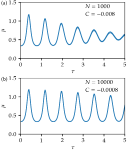
Figure 3: Correlation $\mu$ over time. Simulation with $N=10^{3}$, $C=-8\times 10^{-3}$ (a) and $N=10^{4}$, $C=-8\times 10^{-4}$ (b), $M=512$, $L=20$, $10^{5}$ trajectories, $10^{5}$ time steps. The area between the simulation curves (solid blue lines) denotes the estimated sampling error. The time-step errors are smaller than the line thickness and are not shown on the graph.

Since the center-of mass position is known to spread, one may expect that the on-axis density plotted in Fig. 1 and Fig. 2 might decay purely due to the quantum uncertainty in the final position. Therefore, in Fig. 3, we introduce the dimensionless Glauber second order correlation function, $G^{(2)}\left(z_{1},z_{2}\right)=\left\langle\hat{\psi}^{\dagger}\left(z_{1}\right)\hat{\psi}^{\dagger}\left(z_{2}\right)\hat{\psi}\left(z_{2}\right)\hat{\psi}\left(z_{1}\right)\right\rangle$, and investigate the integrated correlation:

$$\mu=\int G^{(2)}\left(z,z\right)dz/N^{2}.$$ (10)

This integrated correlation function measures the “peakedness” of a spatial distribution, in a way that is independent of the location of the peak. This also decays, although not as strongly as the on-axis density. We conclude that the breather appears to gradually radiate or fragment due to quantum effects with increasing similarity to mean field behaviour as $N\rightarrow\infty$. This is confirmed by an eigenvalue analysis of the first order correlation function, $G^{(1)}\left(z_{1},z_{2}\right)=\left\langle\hat{\psi}^{\dagger}\left(z_{1}\right)\hat{\psi}\left(z_{2}\right)\right\rangle$. The definition of a Bose condensate is that it has a macroscopic occupation Penrose and Onsager (1956)of a single eigenmode of $G^{(1)}$. The transition to a partially fragmented BEC is illustrated in Fig. 4, which shows that six modes dynamically evolve to $>1\%$ occupation by $\tau=5$. This cannot be treated accurately by variational calculations with fewer modes Cosme et al. (2016).

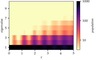
Figure 4: Eigenvalues of the correlation function $G^{(1)}$ over time. Simulation with $N=10^{3}$, $C=-8\times 10^{-3}$ $M=512$, $L=20$, $10^{3}$ trajectories, $10^{5}$ time steps. The graph shows increasing fragmentation with time.

In summary, our results predict continuous quantum fragmentation of higher-order soliton breathers at particle numbers of $N=1000$, with results closer to mean field predictions at $N=10000$. This is readily testable in BEC experiments.