On the Convergence Properties of a $K$-step Averaging Stochastic Gradient Descent Algorithm for Nonconvex Optimization

Abstract

We adopt and analyze a synchronous K-step averaging stochastic gradient descent algorithm which we call K-AVG for solving large scale machine learning problems. We establish the convergence results of K-AVG for nonconvex objectives. Our analysis of K-AVG applies to many existing variants of synchronous SGD. We explain why the K-step delay is necessary and leads to better performance than traditional parallel stochastic gradient descent which is equivalent to K-AVG with $K=1$. We also show that K-AVG scales better with the number of learners than asynchronous stochastic gradient descent (ASGD). Another advantage of K-AVG over ASGD is that it allows larger stepsizes and facilitates faster convergence. On a cluster of $128$ GPUs, K-AVG is faster than ASGD implementations and achieves better accuracies and faster convergence for training with the CIFAR-10 dataset.

1 Introduction

Parallel and distributed processing have been adopted for stochastic optimization to solve large-scale machine learning problems. Efficient parallelization is critical to accelerating long running deep-learning applications. Derived from stochastic gradient descent (SGD), parallel solvers such as synchronous SGD (e.g., Zinkevich et al. (2010) Dekel et al. (2012)) and Asynchronous SGD (ASGD) (e.g., see Dean et al. (2012); Recht et al. (2011)), have been proposed.

Beginning with the seminal paper Robbins and Monro (1951), the convergence properties of SGD and its variants have been extensively studied for the past 50 years (e.g. see Robbins and Siegmund (1971); Bottou (1998); Nemirovski et al. (2009); Shamir and Zhang (2013); Ghadimi and Lan (2013)). The asymptotic optimal convergence rate of SGD was proved by Chung (1954) and Sacks (1958) to be $O(1/N)$ with twice continuously differentiable and strongly convex objectives. $N$ is the number of samples processed. The iteration complexity is $O(1/\sqrt{N})$ for general convex (see Nemirovski et al. (2009)) and nonconvex (see Ghadimi and Lan (2013)) problems. Regarding parallel variants of SGD, Dekel et al. (2012) extend these results to the setting of synchronous SGD with $P$ learners and show that it has convergence rate of $O(1/\sqrt{NP})$ for non-convex objectives, with $N$ being the number of samples processed by each learner. Hogwild! is a lockfree implementation of ASGD, and Recht et al. (2011) prove its convergence for strongly convex problems with theoretical linear speedup over SGD. Downpour is another ASGD implementation with resilience against machine failures Dean et al. (2012). Lian et al. (2015) show that as long as the gradient staleness is bounded by the number of learners, ASGD converges for nonconvex problems. Due to its asynchronous nature that reduces communication cost, ASGD receives much attention in many recent studies.

Although ASGD has the same asymptotic convergence rate as SGD when the staleness of gradient update is bounded, the learning rate assumed for proving ASGD convergence are usually too small for practical purposes. It is also difficult for an ASGD implementation to control the staleness in gradient updates as it is influenced by the relative processing speed of learners and their positions in the communication network. Furthermore, the parameter server presents performance challenges on platforms with many GPUs. On such platforms, a single parameter server oftentimes does not serve the aggregation requests fast enough. A sharded server alleviates the aggregation bottleneck but introduces inconsistencies for parameters distributed on multiple shards. Communication between the parameter server (typically on CPUs) and the learners (on GPUs) is likely to remain a bottleneck in future systems.

We adopt a distributed, bulk-synchronous SGD algorithm that allows delayed gradient aggregation to effectively minimize the communication overhead. We call this algorithm K-step average SGD (K-AVG). Instead of using a parameter server, the learners in K-AVG compute the average of their copies of parameters at regular intervals through global reduction. Rather than relying on asynchrony that reduces communication overhead but has adverse impact on practical convergence, the communication interval $K$ is a parameter in K-AVG. The communication time is amortized among the data samples processed within each interval. On current and emerging computer platforms that support high bandwidth direct communication among GPUs (e.g., GPU-direct), global reduction does not involve CPUs and avoids multiple costly copies through the software layers. Similar averaging approaches have been proposed in the literature, see Hazan and Kale (2014); Johnson and Zhang (2013); Smith et al. (2016); Zhang et al. (2016); Loshchilov and Hutter (2016); Chen et al. (2016); Wang et al. (2017). However, their convergence behavior is not well understood analytically for nonconvex objectives, and it is unclear how they compare with ASGD approaches. This is the part where our major contribution goes to.

We study the convergence behavior of K-AVG and the impact of the number of processors $P$ on convergence. As the abundance of data is critical to the success of most machine learning tasks, training employs increasingly more learners. We show that K-AVG scales better than ASGD with $P$ and K-AVG allows larger stepsizes than ASGD for the same $P$. We also analyze the impact of $K$ on convergence. Since with $K=1$ K-AVG becomes hard-sync SGD, and with larger $K$ K-AVG can stimulate averaging after an epoch or many epochs, our analysis can be applied to many existing variants of synchronous SGD. Finding the optimal length of delay $K_{opt}$ for convergence is of high importance to practitioners. Contrary to popular belief, $K_{opt}$ is oftentimes not $1$ and can be very large for many applications. Thus K-AVG is a good fit for large-scale distributed training as communication may not need to be very frequent for optimal convergence. Our analysis of convergence of K-AVG provides guidelines practitioners to explicitly balance the decrease of communication time and the increase of iterations through an appropriately chosen $K$.

Using an image recognition benchmark, we demonstrate the nice convergence properties of K-AVG in comparison to two popular ASGD implementations: Downpour Dean et al. (2012) and EAMSGD Zhang et al. (2015). In EAMSGD, global gradient aggregation among learners simulates an elastic force that links the parameters they compute with a center variable stored by the parameter server. In both Downpour and EAMSGD, updates to the central parameter server can also have a K-step delay. On our target platform, when $K$ is small, K-AVG significantly reduces the communication time in comparison to Downpour and EAMSGD while achieving similar training and test accuracies. The training time reduction is up to 50%. When $K$ is large, K-AVG achieves much better training and test accuracies than Downpour and EAMSGD after the same amount of data samples are processed. For example, with 128 GPUs, K-AVG is up to about $7$ and $2$-$6$ times faster than Downpour and EAMSGD respectively, and achieves significantly better accuracy.

This rest of the paper is organized as follows: In section 2, we introduce the standard assumptions in optimization theory needed to analyze SGD methods and frequently used notations throughout the paper; In section 3, we formally introduce the K-AVG algorithm, and prove its standard convergence results with fixed and diminishing stepsize. Based on the convergence result, we analyze the scalability of K-AVG and investigate the optimal choice of $K$; In section 4, we present our experimental results to validate our analysis.

2 Preliminaries and notations

In this section, we introduce some standard assumptions used in the analysis of convex and non-convex optimization algorithms and key notations frequently used throughout this paper. We use $\|\cdot\|_{2}$ to denote the $\ell_{2}$ norm of a vector in $\mathbb{R}^{d}$; $\langle\cdot\rangle$ to denote the general inner product in $\mathbb{R}^{d}$. For the key parameters we use:

• $P$ denotes the number of processors;

• $K$ denotes the length of the delay;

• $B_{n}$, $\bar{B}$, or $B$ denotes the size of mini-batch for $n$-th update;

• $\gamma_{n}$, $\bar{\gamma}$, or $\gamma$ denotes the step size for $n$-th update;

• $\xi^{j}_{k,s}$ denotes the i.i.d. realizations of a random variable $\xi$ generated by the algorithm on different processors and in different iterations, especially, $j=1,...,N$, $k=1,...,K$, and $s=1,...,B$.

We study the following optimization problem:

$$\min\limits_{\mathbf{w}\in\mathcal{X}}F(\mathbf{w})$$ (2.1)

where objective function $F:\mathbb{R}^{m}\rightarrow\mathbb{R}$ is continuously differentiable but not necessarily convex over $\mathcal{X}$, and $\mathcal{X}\subset\mathbb{R}^{m}$ is a nonempty open subset. Since our analysis is in a very general setting, $F$ can be understood as both the expected risk $F(\mathbf{w})=\mathbb{E}f(\mathbf{w};\xi)$ or the empirical risk $F(\mathbf{w})=n^{-1}\sum_{i=1}^{n}f_{i}(\mathbf{w})$. As our approach for analysis is built upon smooth objectives, we introduce the following assumptions which are standard and fundamental.

Assumption 1.

The objective function $F:\mathbb{R}^{d}\rightarrow\mathbb{R}$ is continuously differentiable and the gradient function of $F$ is Lipschitz continuous with Lipschitz constant $L>0$, i.e.

$$\big{\|}\nabla F(\mathbf{w})-\nabla F(\widetilde{\mathbf{w}})\big{\|}_{2}\leq L\big{\|}\mathbf{w}-\widetilde{\mathbf{w}}\big{\|}_{2}$$

for all $\mathbf{w}$, $\widetilde{\mathbf{w}}\in\mathbb{R}^{d}$.

This assumption is essential to convergence analysis of our algorithm as well as most gradient based ones. Under such an assumption, the gradient of $F$ serves as a good indicator for how far to move to decrease $F$.

Assumption 2.

The sequence of iterates $\{\mathbf{w}_{j}\}$ is contained in an open set over which $F$ is bounded below by a scalar $F^{*}$.

Assumption 2 requires that objective function to be bounded from below, which guarantees the problem we study is well defined.

Assumption 3.

For any fixed parameter $\mathbf{w}$, the stochastic gradient $\nabla F(\mathbf{w};\xi)$ is an unbiased estimator of the true gradient corresponding to the parameter $\mathbf{w}$, namely,

$$\mathbb{E}_{\xi}\nabla F(\mathbf{w};\xi)=\nabla F(\mathbf{w}).$$

One should notice that the unbiasedness assumption here can be replaced by a weaker version which is called the First Limit Assumption see Bottou et al. (2016) that can still be applied to our analysis. For simplicity, we just assume that the stochastic gradient is an unbiased estimator of the true one.

Assumption 4.

There exist scalars $M\geq 0$ such that,

$$\mathbb{E}_{\xi}\big{\|}\nabla F(\mathbf{w};\xi)\big{\|}_{2}^{2}-\big{\|}\mathbb{E}_{\xi}\nabla F(\mathbf{w};\xi)\big{\|}_{2}^{2}\leq M.$$

Assumption 4 characterizes the variance (second order moments) of the stochastic gradients.

Since all results in this paper are based on the four assumptions above, we present them with no further mention in the following literature.

3 Main results

We present the distributed K-AVG algorithm as follows:

initialize $\widetilde{\mathbf{w}}_{1}$;

for $n=1,...,N$ do

       Processor $P_{j}$, $j=1,\dots,P$ do concurrently:

       set $\mathbf{w}_{n}^{j}=\widetilde{\mathbf{w}}_{n}$ ;

       for $k=1,...,K$ do

            

            randomly sample a mini-batch of size $B_{n}$ and update:

$$\mathbf{w}_{n+k}^{j}=\mathbf{w}_{n+k-1}^{j}-\frac{\gamma_{n}}{B_{n}}\sum\limits_{s=1}^{B_{n}}\nabla F(\mathbf{w}_{n+k-1}^{j};\xi_{k,s}^{j})$$

       end for

      Synchronize $\widetilde{\mathbf{w}}_{n+1}=\frac{1}{P}\sum\limits_{j=1}^{P}\mathbf{w}_{n+K}^{j}$;

      

end for

Algorithm 1 K-step average stochastic gradient descent algorithm

Note that traditional parallel SGD algorithm is equivalent to K-AVG with $K=1$, as synchronization is required after each local update. However, K-AVG relaxes this requirement and allows for $K$ individual updates before synchronization. Thus, K-AVG is a more general synchronous algorithm that contains parallel SGD. Surprisingly, as we show both analytically (section 3.4) and experimentally (section 4.2), more frequent synchronization does not always result in faster convergence for nonconvex objectives.

3.1 Convergence of K-AVG

In the following theorem, we prove an upper bound on the expected average squared gradient norms, which serve as a metric to measure the convergence rate for nonconvex objectives.

Theorem 3.1.

(Nonconvex objective, fixed stepsize, and fixed batch size) Suppose that Algorithm 1 is run with a fixed stepsize $\gamma_{n}=\bar{\gamma}$, a fixed batch size $B_{n}=\bar{B}$ satisfying

$$1\geq\frac{L^{2}\bar{\gamma}^{2}(K+1)(K-2)}{2}+L\bar{\gamma}K,~{}~{}~{}and~{}~{}~{}1-\delta\geq L^{2}\bar{\gamma}^{2}$$ (3.1)

with some constant $0<\delta<1$. Then the expected average squared gradient norms of $F$ satisfy the following bounds for all $N\in\mathbb{N}$:

$$\frac{1}{N}\mathbb{E}\sum\limits_{j=1}^{N}\big{\|}\nabla F(\widetilde{\mathbf{w}}_{j})\big{\|}_{2}^{2}\leq\Big{[}\frac{2(F(\widetilde{\mathbf{w}}_{1})-F^{*})}{N(K-1+\delta)\bar{\gamma}}+\frac{LK\bar{\gamma}M}{\bar{B}(K-1+\delta)}\Big{(}\frac{K}{P}+\frac{L(2K-1)(K-1)\bar{\gamma}}{6}\Big{)}\Big{]},$$ (3.2)

The proof of Theorem 3.1 can be found in section 6.1. An immediate observation from (3.2) is that the expected average squared gradient norms of $F$ converges to some nonzero constant as $N\rightarrow\infty$. The first term $\frac{2(F(\widetilde{\mathbf{w}}_{1})-F^{*})}{N(K-1+\delta)\bar{\gamma}}$ reflects the distance from initial weight to the solution. It eventually goes to zero as the number of iterations goes to infinity. The second term $\frac{LK\bar{\gamma}M}{\bar{B}(K-1+\delta)}\Big{(}\frac{K}{P}+\frac{L(2K-1)(K-1)\bar{\gamma}}{6}\Big{)}$ is not affected by the iteration number. Compared with sequential SGD (see section 4.3 in Bottou et al. (2016)), this term is scaled by the batch size $1/\bar{B}$, and $1/P$ or $\frac{L(2K-1)(K-1)\bar{\gamma}}{6}$, which means larger batch size and smaller stepsize, more learners or more frequent averaging tend to reduce this term. Mini-batch method as a variance reduction technique explains the appearance of $\bar{B}$. Parallelization of this algorithm contributes to the scaling factor $1/P$. However, when $P$ is large enough to make $\frac{L(2K-1)(K-1)\bar{\gamma}}{6}$ dominates $K/P$, the effect of parallelization is not ideal as one may expect.

The rates of convergence (also referred as iteration complexity) after $N$ step updates are established in the following corollary which originates from Theorem 3.1.

Corollary 3.1.

Under the condition of Theorem 3.1, take

$$\bar{\gamma}=\sqrt{\frac{(F(\widetilde{\mathbf{w}}_{1})-F^{*})\bar{B}P}{LMK^{2}N}}$$ (3.3)

Then for any

$$N\geq\frac{(F(\widetilde{\mathbf{w}}_{1})-F^{*})L\bar{B}P}{M}\Big{(}\frac{P^{2}}{K^{2}}\bigvee 1\Big{)},$$

the following bound is achieved

$$\mathbb{E}\frac{1}{N}\sum\limits_{n=1}^{N}\big{\|}\nabla F(\widetilde{\mathbf{w}}_{n})\big{\|}_{2}^{2}\leq\Big{(}\frac{4K}{K-1+\delta}\Big{)}\sqrt{\frac{(F(\widetilde{\mathbf{w}}_{1})-F^{*})LM}{\bar{B}P}}*\frac{1}{\sqrt{N}}.$$ (3.4)

The proof of Corollary 3.1 can be found in section 6.3. Condition (3.3) and bound (3.4) imply when the number of updates $N$ is large enough, K-AVG eventually achieves a similar rate of convergence as classical SGD method for nonconvex objectives. Indeed, the rate of convergence of classical SGD methods is $N^{-1/2}$ after $N$ samples processed. Note that $N$ updates in K-AVG means that $N*K*B*P$ samples have been processed. Taking a closer look at bound in (3.4), the right hand side is of the order $O((N*B*P)^{-1/2})$. K-AVG loses a factor of $1/\sqrt{K}$ as a result of communication saving. However, this doesn’t mean that the smaller $K$ the better. Since there is an extra multiplicative factor $\frac{4K}{K-1+\delta}$ which is monotone decreasing with respect to $K$. We will have a more detailed discussion on the choice of $K$ in section 3.4.

Deploying diminishing stepsizes and/or dynamic batch sizes makes the expected average squared gradient norms converge to zero for non-convex optimization. In the following theorem, we establish the convergence result under such conditions.

Theorem 3.2.

(Nonconvex objective, diminishing step size, and growing batch size) Suppose that Algorithm 1 is run with diminishing step size $\gamma_{j}$, and growing batch size $B_{j}$ satisfying

$$1\geq\frac{L^{2}\bar{\gamma}_{j}^{2}(K+1)(K-2)}{2}+L\bar{\gamma}_{j}K,~{}~{}~{}~{}and~{}1-\delta\geq L^{2}\gamma_{j}^{2}$$ (3.5)

with some constant $0<\delta<1$. Then the weighted average squared gradient norms satisfies

$$\mathbb{E}\sum\limits_{j=1}^{N}\frac{\gamma_{j}}{\sum_{j=1}^{N}\gamma_{j}}\big{\|}\nabla F(\widetilde{\mathbf{w}}_{j})\big{\|}^{2}_{2}$$ (3.6)

$$\leq\frac{2(F(\widetilde{\mathbf{w}}_{1})-F^{*})}{(K-1+\delta)\sum_{j=1}^{N}\gamma_{j}}+\sum\limits_{j=1}^{N}\frac{LK\gamma_{j}^{2}M}{B_{j}(K-1+\delta)\sum_{j=1}^{N}\gamma_{j}}\Big{(}\frac{K}{P}+\frac{L(2K-1)(K-1)\gamma_{j}}{6}\Big{)}$$

Especially, if

$$\lim\limits_{N\rightarrow\infty}\sum\limits_{j=1}^{N}\gamma_{j}=\infty,~{}~{}\lim\limits_{N\rightarrow\infty}\sum\limits_{j=1}^{N}\frac{K\gamma_{j}^{2}}{PB_{j}}<\infty,~{}~{}\lim\limits_{N\rightarrow\infty}\sum\limits_{j=1}^{N}\gamma_{j}^{3}<\infty,$$ (3.7)

Then

$$\mathbb{E}\sum\limits_{j=1}^{N}\frac{\gamma_{j}}{\sum_{j=1}^{N}\gamma_{j}}\big{\|}\nabla F(\widetilde{\mathbf{w}}_{j})\big{\|}^{2}_{2}\rightarrow 0,~{}as~{}N\rightarrow\infty.$$

The proof of Theorem 3.2 can be found in section 6.2. As we can see, by adopting a diminishing sequence of stepsizes instead of a fixed one, the expected average squared gradient norms of K-AVG converges to $0$ instead of a nonzero constant.

3.2 K-AVG allows for larger stepsize than ASGD

Compared with the classical stepsize schedule for both sequential SGD (proposed by Robbins and Monro (1951)) and ASGD:

$$\sum\limits_{j=1}^{\infty}\gamma_{j}=\infty,~{}\sum\limits_{j=1}^{\infty}\gamma_{j}^{2}<\infty;$$

the stepsize schedule proposed in (3.7) turns out to allow larger choices of $\gamma_{j}$. On one hand, $\sum_{j=1}^{\infty}\gamma^{3}_{j}<\infty$ itself is a much more relaxed constrain compared with $\sum_{j=1}^{\infty}\gamma^{2}_{j}<\infty$. On the other hand, as a byproduct of parallelization, when $P$ is large, $\sum_{j=1}^{\infty}\gamma^{2}_{j}/B_{j}P$ also allows larger choice of $\gamma_{j}$. Intuitively, averaging acts as a variance reduction and leads to relaxation of larger stepsize constrain. In our experiments (section 4.1), larger stepsizes work well in K-AVG but can result in divergence in popular ASGD implementations.

3.3 Scalability comparison of K-AVG against ASGD

We analyze the bound on expected average squared gradient norms in (3.2) to show K-AVG algorithm scales better with $P$ than ASGD. We first establish the following theorem on the scalability of K-AVG.

Theorem 3.3.

Under the condition of Theorem 3.1, K-AVG scales better than ASGD.

Proof.

In ASGD, one key parameter is the maximum staleness, generally assumed to be upper bounded by the number of processors, i.e. $P$ in K-AVG. With fixed stepsize, the expected average gradient norms is (see also Lian et al. (2015), Theorem 3) is

$$\mathbb{E}\frac{1}{N}\sum\limits_{n=1}^{N}\big{\|}\nabla F(\widetilde{\mathbf{w}}_{n})\big{\|}_{2}^{2}\leq\Big{[}\frac{C_{0}(F(\widetilde{\mathbf{w}}_{1})-F^{*})}{N\bar{\gamma}}+\frac{C_{1}L^{2}\bar{\gamma}^{2}M^{2}P}{2\bar{B}}\Big{]}.$$ (3.8)

where $C_{0}$ and $C_{1}$ are constants independent of $P$.

Compared with the bound in (3.2),

$$\frac{1}{N}\mathbb{E}\sum\limits_{j=1}^{N}\big{\|}\nabla F(\widetilde{\mathbf{w}}_{j})\big{\|}_{2}^{2}\leq\Big{[}\frac{2(F(\widetilde{\mathbf{w}}_{1})-F^{*})}{N(K-1+\delta)\bar{\gamma}}+\frac{LK\bar{\gamma}M}{\bar{B}(K-1+\delta)}\Big{(}\frac{K}{P}+\frac{L(2K-1)(K-1)\bar{\gamma}}{6}\Big{)}\Big{]}$$

$P$ serves as a scaling factor in the denominator, which implies K-AVG scales better than asynchronization. ∎

The comparison of practical scalability between K-AVG and ASGD implementations is shown in section 4.1.

3.4 Optimal $K$ for convergence is not always $1$

Unlike convex optimization problems where all learners converge to the same optimum, different learners may converge to different local optimums in nonconvex case. As a consequence, the frequency of averaging for nonconvex problems may be different from that of convex cases intuitively. Zhang et al. (2016) expressed the same concern, their experimental results showed that periodic averaging tends to improve the solution quality. Contrary to popular belief that more frequent averaging i.e. smaller $K$ speeds up convergence, we show that the optimal frequency $K$ for convergence is not always $1$. We consider the case that the amount of samples processed $N*K$ is constant, which means that the computational time remains as a constant given a fixed number of processors. If every other parameter stays the same, larger $K$ means longer delay and fewer updates of global parameter $\widetilde{\mathbf{w}}_{n}$. The following theorem discusses the impact and optimal choice of $K$ in K-AVG under such an assumption.

Theorem 3.4.

Let $S=N*K$ be a constant. Suppose that Algorithm 1 is run with a fixed stepsize $\gamma_{n}=\bar{\gamma}$, a fixed batch size $B_{n}=\bar{B}$ satisfying

$$1\geq\frac{L^{2}\bar{\gamma}^{2}(K+1)(K-2)}{2}+L\bar{\gamma}K,~{}~{}~{}1-\delta\geq L^{2}\bar{\gamma}^{2}$$

with some constant $0<\delta<1$. If

$$\frac{(1-\delta)(F(\widetilde{\mathbf{w}}_{1})-F^{*})}{S\bar{\gamma}\delta}>\frac{(3\delta-1)L\bar{\gamma}M}{2\delta P\bar{B}}+\frac{L^{2}\bar{\gamma}^{2}M}{3\bar{B}}.$$ (3.9)

Then the optimal choice of $K$ is greater than $1$.

Proof.

Under the assumption $S=N*K$, we can rewrite the bound (3.2) as

$$\frac{1}{N}\mathbb{E}\sum\limits_{j=1}^{N}\big{\|}\nabla F(\widetilde{\mathbf{w}}_{j})\big{\|}_{2}^{2}\leq\Big{[}\frac{2(F(\widetilde{\mathbf{w}}_{1})-F^{*})K}{S(K-1+\delta)\bar{\gamma}}+\frac{LK\bar{\gamma}M}{\bar{B}(K-1+\delta)}\Big{(}\frac{K}{P}+\frac{L(2K-1)(K-1)\bar{\gamma}}{6}\Big{)}\Big{]}.$$ (3.10)

To move on, we set

$$B(K):=\Big{(}\alpha+\beta K+\eta(2K-1)(K-1)\Big{)}\Big{(}\frac{K}{K-1+\delta}\Big{)},$$

where

$$\alpha=\frac{2(F(\widetilde{\mathbf{w}}_{1})-F^{*})}{S\bar{\gamma}},~{}\beta=\frac{L\bar{\gamma}M}{P\bar{B}},~{}\eta=\frac{L^{2}\bar{\gamma}^{2}M}{6\bar{B}}.$$

To minimize the right hand side of (3.10), it is equivalent to solve the following integer program

$$K^{*}=\operatorname{argmin}\limits_{K\in\mathbb{N}^{*}}B(K),$$

which can be very hard. Meanwhile, one should notice that $K^{*}$ depends on some unknown quantities such as $L$, $M$ and $(F(\widetilde{\mathbf{w}}_{1})-F^{*})$. Instead, we investigate the monotonicity of $B(K)$. It is easy to check that $\Big{(}\alpha+\beta K+\eta(2K-1)(K-1)\Big{)}$ is monotone increasing for all $K\geq 1$, and $\Big{(}\frac{K}{K-1+\delta}\Big{)}$ is monotone decreasing for $K\geq 1$. Thus, there exists a unique $K^{*}$. Then a sufficient condition for $K^{*}>1$ is that $B(2)<B(1)$, which implies

$$\frac{1-\delta}{2\delta}\alpha>\frac{3\delta-1}{2\delta}\beta+3\eta.$$

∎

The meaning of Theorem 3.4 is that it indicates when it comes to nonconvex optimization, more frequent averaging is not necessary. The sufficient condition (3.9) implies that larger value of $\big{(}F(\widetilde{\mathbf{w}}_{1})-F^{*}\big{)}$ requires larger $K$ thus longer delay to decrease the bound in (3.10). The intuition is that if the initial weight is too far away from $F^{*}$, then less frequent synchronizations can lead to faster convergence rate. Less frequent averaging implies higher variance in general. It is quite reasonable to think that if it is still far away from the solution, a stochastic gradient direction with larger variance may be preferred.

As we have already mentioned in the proof, optimal value $K^{*}$ depends on quantities such as $L$, $M$, and $(F(\widetilde{\mathbf{w}}_{1})-F^{*})$ which are unknown to us in practice. Therefore, to obtain a concrete $K^{*}$ in practice is not so realistic. Note that when $K^{*}>1$ doesn’t necessarily mean that $K^{*}$ is very close to $1$. In our experiments (see section 4), $K^{*}$ can be as large as $16$ or $32$ in some situation.

4 Experiments

We conduct experiments to validate our analysis on the scalability of K-AVG vs. ASGD implementations, the optimal delay in averaging ( optimal value of $K$), the convergence comparison with the sequential algorithm, i.e., SGD, and the comparison of the learning rates allowed with ASGD.

In our application gradient descent is implemented with Torch, and the communication is implemented using CUDA-aware openMPI 2.0 through the mpiT library. All implementations use the cuDNN library for forward propagation and backward propagation. Our experiments are done on a cluster of 32 Minsky nodes interconnected with Infiniband. Each node is an IBM S822LC system containing 2 Power8 CPUs with 10 cores each, and 4 NVIDIA Tesla P100 GPUs.

We experiment with the CIFAR-10 Krizhevsky and Hinton (2009) data set using the vgg and nin models. CIFAR-10 contains $50,000$ training images and $10,000$ test images, each associated with $1$ out of $10$ possible labels.

4.1 Comparison with ASGD

Theorem 3.3 shows that the convergence bound of K-AVG is not affected much by the scaling of $P$ but rather by $K$. On the contrary, the convergence bound of ASGD increases linearly with $P$. Thus we expect poorer convergence behavior of ASGD implementations at large $P$ in comparison with K-AVG.

Figures 2 and  2 compare the performance of K-AVG with two ASGD implementations, Downpour and EAMSGD, for two neural networks, vgg Simonyan and Zisserman (2014) and nin Lin et al. (2013), respectively. We use $P=8,16,32,64$ and $128$ learners, and show the test accuracies. All implementations use the same initial learning rate ($\gamma_{0}=1$) and learning rate adaptation schedule (reduce $\gamma$ by half after 50 epochs). The batch size is fixed at $\bar{B}=16$. We run for 600 epochs with $K=16$ for K-AVG.

In both figures, K-AVG always achieves better test accuracy than Downpour and EAMSGD. The test accuracies for Downpour and EAMSGD decreases as $P$ increases (the effect is more pronounced for vgg). When $P$ reaches 128, the accuracies of Downpour and EAMSGD both degrade to around 10%, i.e, random guess. The ASGD implementations do not converge with $\gamma_{0}=1$ at $P=128$.

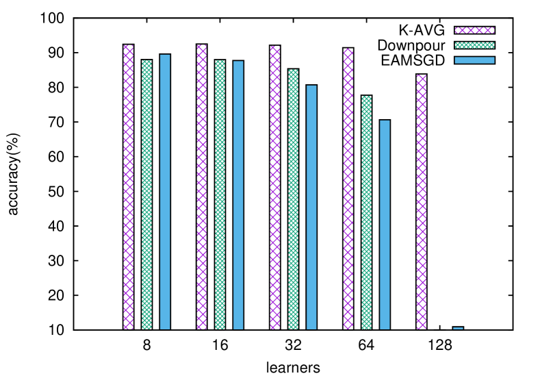
Figure 1: Scaling with vgg

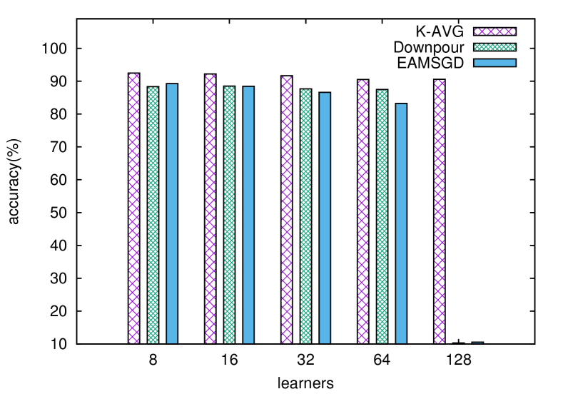
Figure 2: Scaling with nin

When we set the initial learning rate $\gamma_{0}=0.1$, Downpour achieves around 80% and 87% test accuracies for vgg and nin, respectively; EAMSGD still does not converge.

K-AVG achieves better test accuracy than ASGD implementations, and in our experiment it is also faster. We measure wall-clock times for all implementations after 600 epochs. Naturally for K-AVG, $K$ impacts the ratio of communication vs. computation. We still use $K=16$.

Figures 4 and 4 show the speedups of K-AVG over Downpour and EAMSGD, with vgg and nin, respectively. In Figure 4, when $P=8$, the ASGD implementations are slightly faster than K-AVG. As $P$ increases, the speedup increases. When $P=128$, the speedups are around 2.5 and 2.6 over Downpour and EAMSGD, respectively. Similar behavior is observed in Figure 4 for nin.

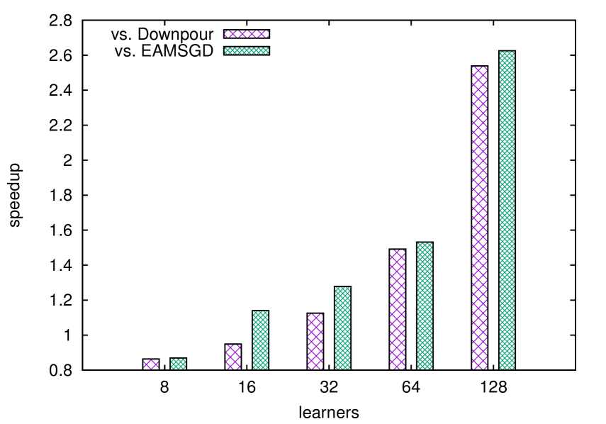
Figure 3: Speedup of K-AVG over ASGD implementations with vgg

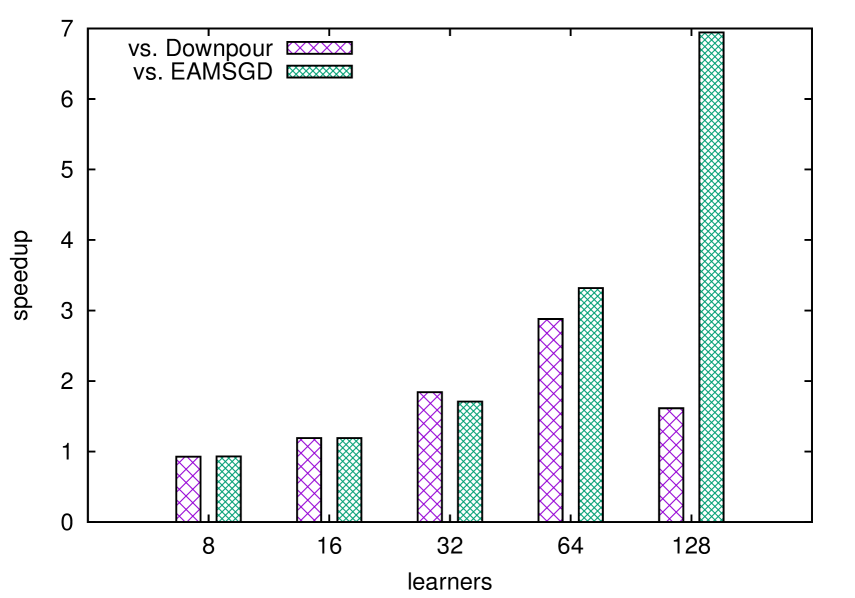
Figure 4: Speedup of K-AVG over ASGD implementations with nin

4.2 The optimal delay in averaging for K-AVG

For K-AVG, $K$ regulates its behavior. From the execution time perspective, larger $K$ results in fewer communications to process a given number of data samples. From the convergence perspective, smaller $K$ reduces the variances among learners. In the extreme case where $K=1$, K-AVG is equivalent to synchronous parallelization of SGD. People tend to think that smaller $K$ results in faster convergence in terms of number of data samples processed. As discussed in Section 3.4, there are scenarios where $K_{opt}$ is not 1.

We evaluate the convergence behavior of K-AVG with different $K$ values for vgg and nin. We experiment with $K=1,2,4,16,32$, and $64$. Figures 6 and 6 show the test accuracies achieved after 600 epochs for $P=8,16,32,64$, and $128$, for vgg and nin, respectively. Again we use the initial $\gamma_{0}$=1, and after every 50 epochs, $\gamma$ is reduced by half. The batch size is fixed as $\bar{B}=32$.

In Figure 6, strikingly, none of the experiments show the optimal value of $K$ for K-AVG is 1. $K_{opt}$ ranges from 32 (when $P=8$) farthest away from 1, to 2 (when $P=64$), closest to 1. In this set of experiments, as $P$ increases, $K_{opt}$ tends to decrease. Also with smaller $P$, K-AVG is more forgiving in terms of the choices of $K$. For example, when $P=8$, test accuracies for different $K$ are similar. With larger $P$, however, choosing a $K$ that is too large has severe punishing consequences. For example, when $P=128$, $K_{opt}=4$, and the test accuracy degrades rapidly with the increase of $K$ beyond 4.

In Figure 6, almost all experiments show $K_{opt}$=1. The exception is with $p=8$, and the accuracy is slightly higher (by 0.27%) at $K=8$ than $K=1$. Again we see for small $p$ the choices of $K$ is not critical, while for large $p$ the degradation in accuracy is rapid with the increase of $K$ beyond $K_{opt}$.

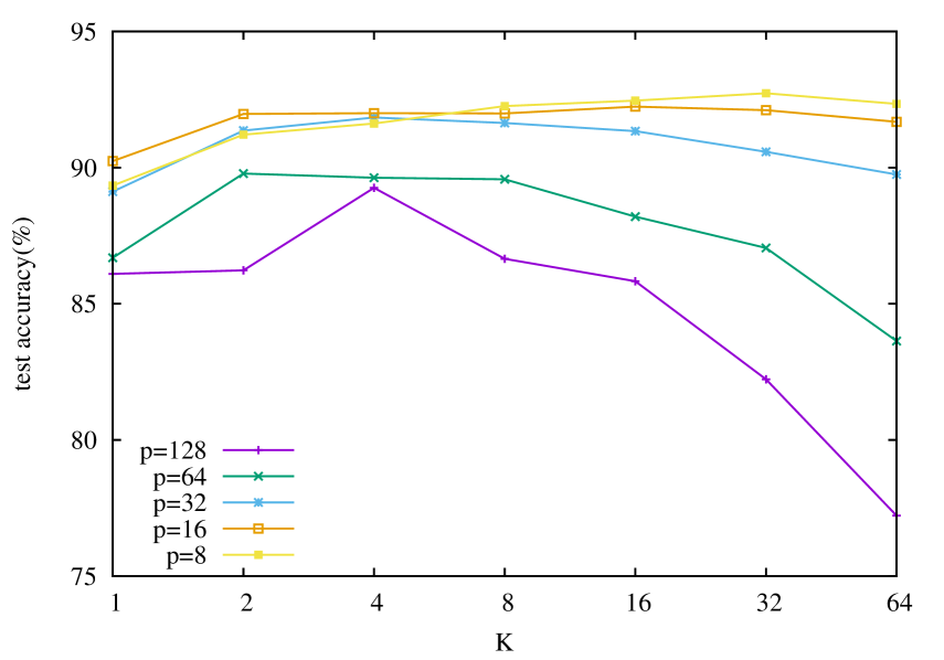
Figure 5: Test accuracy with different $K$

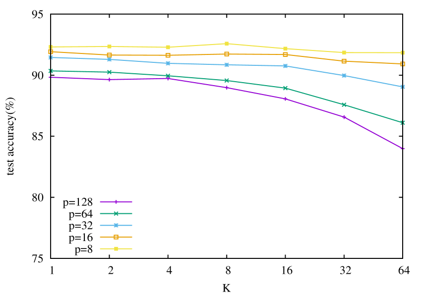
Figure 6: Test accuracy with different $K$

Since in our experiments the same hyper-parameters are used for vgg and nin, it is likely that the Lipschitz constant $L$ largely determines the differences in $K_{opt}$ between the two cases.

4.3 Convergence comparison with SGD

We compare the performance of K-AVG against the sequential implementation, that is, SGD. We evaluate the test accuracies achieved and the wall clock time used.

Figure 8 shows the accuracy gap between K-AVG and SGD. With $8$ and $16$ learners, K-AVG is slightly worse than sequential SGD for vgg but better than nin. K-AVG and SGD achieve comparable accuracies with 32 learners. As the number of learners reaches 64 and 128, significant accuracy degradation, up to 8.8% is observed for vgg. Interestingly, the accuracy degradation for nin is still within 1.3% with 128 learners.

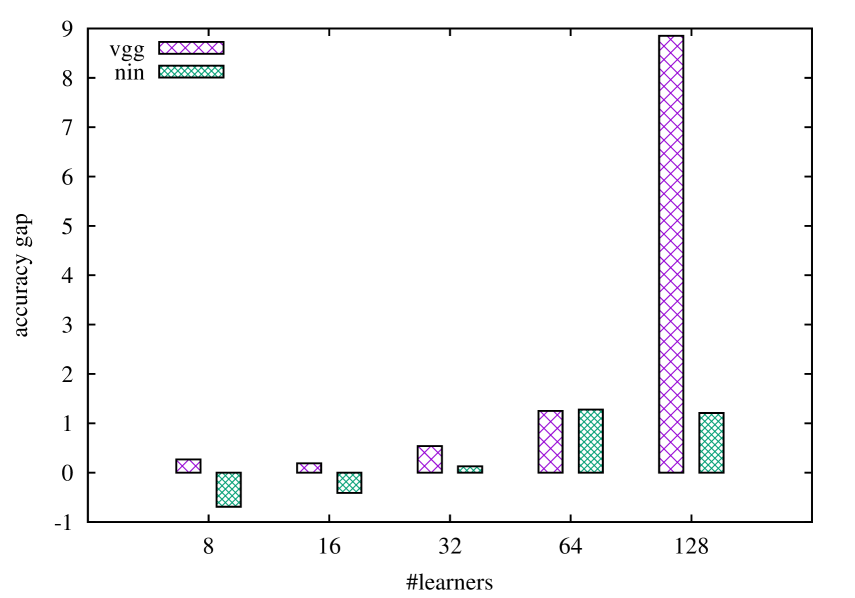
Figure 7: Accuracy gap

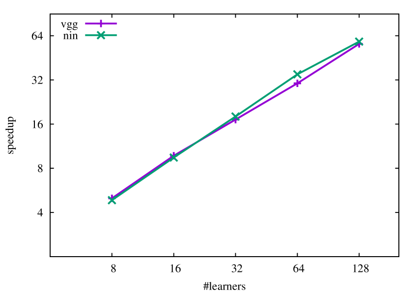
Figure 8: Epoch time speedup

Figure 8 shows the epoch time speedup of K-AVG against SGD with 8, 16, 32, 64, and 128 learners. With 8 learners, the speedups for vgg and nin are 4.9, and 4.8, respectively. With 128 learners, the speedups for vgg and nin are 56.3 and 58.3, respectively. Since twice as many epochs are run for K-AVG in comparison to SGD, the wallclock time speedups are half of these numbers. This means linear speedup is achieved.

5 Conclusion

In this paper, we adopt and analyze K-AVG for solving large scale machine learning problems with nonconvex objectives. We establish the convergence results of K-AVG under both fixed and diminishing stepsize, and show that with a properly chosen sequence of stepsizes, K-AVG achieves similar convergence rate consistent with its sequential counterpart. We show that K-AVG scales better than ASGD with properly chosen $K$ when $P$ is large. K-AVG allows larger stepsizes that still guarantees convergence while ASGD may fail to converge. Contrary to popular belief, we show that the length of delay to average learning parameters among parallel learners is not necessarily to be $1$. Although, a proper choice of $K_{opt}$ remains unknown, we analytically explain the dependence of $K_{opt}$ on other parameters which we hope can serve as a users’ guide in practical implementations.

6 Proofs

6.1 Proof of Theorem 3.1

Proof.

We denote $\widetilde{\mathbf{w}}_{\alpha}$ as the $\alpha$-th global update in K-AVG, and denote $\mathbf{w}^{j}_{\alpha+t}$ as $t$-th local update on processor $j$. The $(\alpha+1)$-th global average can be written as

$$\widetilde{\mathbf{w}}_{\alpha+1}=\frac{1}{P}\sum\limits_{j=1}^{P}\mathbf{w}_{\alpha+K}^{j}=\frac{1}{P}\sum\limits_{j=1}^{P}\Big{[}\mathbf{w}_{\alpha}^{j}-\sum\limits_{t=0}^{K-1}\frac{\gamma_{t}}{B}\sum\limits_{s=1}^{B}\nabla F(\mathbf{w}_{\alpha+t}^{j};\xi_{t,s}^{j})\Big{]},$$

according to our algorithm, the random variables $\xi_{t,s}^{j}$ are i.i.d. for all $t=0,...,K-1$, $s=1,...,B$, and $j=1,...,P$.

$$F(\widetilde{\mathbf{w}}_{\alpha+1})-F(\widetilde{\mathbf{w}}_{\alpha}) \leq\Big{\langle}\nabla F(\widetilde{\mathbf{w}}_{\alpha}),\widetilde{\mathbf{w}}_{\alpha+1}-\widetilde{\mathbf{w}}_{\alpha}\Big{\rangle}+\frac{L}{2}\big{\|}\widetilde{\mathbf{w}}_{\alpha+1}-\widetilde{\mathbf{w}}_{\alpha}\big{\|}_{2}^{2}$$ (6.1)

$$\leq-\Big{\langle}\nabla F(\widetilde{\mathbf{w}}_{\alpha}),\frac{1}{P}\sum\limits_{j=1}^{P}\sum\limits_{t=0}^{K-1}\frac{\gamma_{t}}{B}\sum\limits_{s=1}^{B}\nabla F(\mathbf{w}_{\alpha+t}^{j};\xi_{t,s}^{j})\Big{\rangle}$$ (6.2)

$$+\frac{L}{2}\Big{\|}\frac{1}{P}\sum\limits_{j=1}^{P}\sum\limits_{t=0}^{K-1}\frac{\gamma_{t}}{B}\sum\limits_{s=1}^{B}\nabla F(\mathbf{w}_{\alpha+t}^{j};\xi_{t,s}^{j})\Big{\|}_{2}^{2}.$$ (6.3)

Under the assumption that a constant stepsize is implemented within each inner parallel step, i.e. $\gamma_{t}=\gamma$, for $t=0,...,K-1$, one can immediately simplify the above inequality as

$$F(\widetilde{\mathbf{w}}_{\alpha+1})-F(\widetilde{\mathbf{w}}_{\alpha}) \leq-\frac{\gamma}{PB}\sum\limits_{j=1}^{P}\sum\limits_{t=0}^{K-1}\sum\limits_{s=1}^{B}\Big{\langle}\nabla F(\widetilde{\mathbf{w}}_{\alpha}),\nabla F(\mathbf{w}_{\alpha+t}^{j};\xi_{t,s}^{j})\Big{\rangle}$$ (6.4)

$$+\frac{L\gamma^{2}}{2P^{2}B^{2}}\Big{\|}\sum\limits_{j=1}^{P}\sum\limits_{t=0}^{K-1}\sum\limits_{s=1}^{B}\nabla F(\mathbf{w}_{\alpha+t}^{j};\xi_{t,s}^{j})\Big{\|}_{2}^{2}.$$ (6.5)

The goal here is to investigate the expectation of $F(\widetilde{\mathbf{w}}_{\alpha+1})-F(\widetilde{\mathbf{w}}_{\alpha})$ over all random variables $\xi_{t,s}^{j}$. Under the unbiased estimation Assumption 3, by taking the overall expectation we can immediately get

$$\mathbb{E}\frac{1}{B}\sum\limits_{s=1}^{B}\nabla F(\mathbf{w}_{\alpha+t}^{j};\xi_{t,s}^{j})=\mathbb{E}\Big{[}\frac{1}{B}\sum\limits_{s=1}^{B}\mathbb{E}_{\xi^{j}_{t,s}}\nabla F(\mathbf{w}_{\alpha+t}^{j};\xi_{t,s}^{j}|\mathbf{w}_{\alpha+t}^{j})\Big{]}=\mathbb{E}\nabla F(\mathbf{w}_{\alpha+t}^{j}).$$

for fixed $j$ and $t$. Here we abuse the expectation notation $\mathbb{E}$ a little bit. Throughout this proof, $\mathbb{E}$ always means taking the overall expectation. We will frequently use the above iterative conditional expectation trick in the following analysis. As a result, we can drop the summation over $s$ due to an averaging factor $B$ in the dominator of (6.4). Next, we show how to get rid of the summation over $j$. Recall that $\mathbf{w}^{j}_{\alpha+1}=\widetilde{\mathbf{w}}_{\alpha}-\frac{\gamma}{B}\sum_{s=1}^{B}\nabla F(\widetilde{\mathbf{w}}_{\alpha};\xi^{j}_{0,s})$. Obviously, $\mathbf{w}_{\alpha+1}^{j}$, $j=1,...,P$ are i.i.d. for fixed $\widetilde{\mathbf{w}}_{\alpha}$ because $\xi_{0,s}^{j}$, $j=1,...,P$, $s=1,...,B$ are i.i.d. Similarly, $\mathbf{w}^{j}_{\alpha+2}=\mathbf{w}^{j}_{\alpha+1}-\frac{\gamma}{B}\sum_{s=1}^{B}\nabla F(\mathbf{w}^{j}_{\alpha+1};\xi^{j}_{1,s})$, $j=1,...,P$ are i.i.d. due to the fact that $\mathbf{w}_{\alpha+1}^{j}$’s are i.i.d., $\xi_{1,s}^{j}$’s are i.i.d., and $\mathbf{w}_{\alpha+1}^{j}$’s are independent from $\xi_{1,s}^{j}$’s. By induction, one can easily show that for each fixed $t$, $\mathbf{w}_{\alpha+t}^{j}$, $j=1,...,P$ are i.i.d. Thus for each fixed $t$

$$\frac{1}{P}\sum\limits_{j=1}^{P}\mathbb{E}\nabla F(\mathbf{w}_{\alpha+t}^{j})=\mathbb{E}\nabla F(\mathbf{w}_{\alpha+t}^{j}).$$

We can therefore get rid of the summation over $j$ as well in (6.4). By taking the overall expectation on both sides of (6.4) and (6.5), we have

$$\mathbb{E}F(\widetilde{\mathbf{w}}_{\alpha+1})-F(\widetilde{\mathbf{w}}_{\alpha}) \leq-\gamma\sum\limits_{t=0}^{K-1}\mathbb{E}\Big{\langle}\nabla F(\widetilde{\mathbf{w}}_{\alpha}),\nabla F(\mathbf{w}_{\alpha+t}^{j})\Big{\rangle}$$ (6.6)

$$+\frac{L\gamma^{2}}{2P^{2}B^{2}}\mathbb{E}\Big{\|}\sum\limits_{j=1}^{P}\sum\limits_{t=0}^{K-1}\sum\limits_{s=1}^{B}\nabla F(\mathbf{w}_{\alpha+t}^{j};\xi_{t,s}^{j})\Big{\|}_{2}^{2}.$$ (6.7)

We are going to bound (6.6) and (6.7) respectively. Obviously (we treat $\widetilde{\mathbf{w}}_{\alpha}$ as a constant vector at this moment),

$$-\gamma\sum\limits_{t=0}^{K-1}\mathbb{E}\Big{\langle}\nabla F(\widetilde{\mathbf{w}}_{\alpha}),\nabla F(\mathbf{w}_{\alpha+t}^{j})\Big{\rangle} =-\frac{\gamma}{2}\sum\limits_{t=0}^{K-1}\Big{(}\big{\|}\nabla F(\widetilde{\mathbf{w}}_{\alpha})\big{\|}_{2}^{2}+\mathbb{E}\big{\|}\nabla F(\mathbf{w}_{\alpha+t}^{j})\big{\|}_{2}^{2}\Big{)}$$ (6.8)

$$+\frac{\gamma}{2}\sum\limits_{t=0}^{K-1}\mathbb{E}\big{\|}\nabla F(\mathbf{w}_{\alpha+t}^{j})-\nabla F(\widetilde{\mathbf{w}}_{\alpha})\big{\|}_{2}^{2}$$

$$\leq-\frac{(K+1)\gamma}{2}\big{\|}\nabla F(\widetilde{\mathbf{w}}_{\alpha})\big{\|}_{2}^{2}-\frac{\gamma}{2}\sum\limits_{t=1}^{K-1}\mathbb{E}\big{\|}\nabla F(\mathbf{w}_{\alpha+t}^{j})\big{\|}_{2}^{2}$$

$$+\frac{L^{2}\gamma}{2}\sum\limits_{t=1}^{K-1}\mathbb{E}\big{\|}\mathbf{w}_{\alpha+t}^{j}-\widetilde{\mathbf{w}}_{\alpha}\big{\|}_{2}^{2},$$

where we used the fact that $\widetilde{\mathbf{w}}_{\alpha}^{j}=\widetilde{\mathbf{w}}_{\alpha}$, for $j=1,...,P$ for the last term and the assumption that gradient $\nabla F$ is Lipschitz continuous. Note that

$$\mathbb{E}\big{\|}\mathbf{w}_{\alpha+t}^{j}-\widetilde{\mathbf{w}}_{\alpha}\big{\|}_{2}^{2} =\frac{\gamma^{2}}{B^{2}}\mathbb{E}\big{\|}\sum\limits_{i=0}^{t-1}\sum\limits_{s=1}^{B}\nabla F(\mathbf{w}_{\alpha+i}^{j};\xi_{i,s}^{j})\big{\|}_{2}^{2}\leq\frac{t\gamma^{2}}{B^{2}}\mathbb{E}\sum\limits_{i=0}^{t-1}\big{\|}\sum\limits_{s=1}^{B}\nabla F(\mathbf{w}_{\alpha+i}^{j};\xi_{i,s}^{j})\big{\|}_{2}^{2}$$

$$=\frac{t\gamma^{2}}{B^{2}}\mathbb{E}\sum\limits_{i=0}^{t-1}\big{\|}\sum\limits_{s=1}^{B}\big{(}\nabla F(\mathbf{w}_{\alpha+i}^{j};\xi_{i,s}^{j})-\nabla F(\mathbf{w}_{\alpha+i}^{j})+\nabla F(\mathbf{w}_{\alpha+i}^{j})\big{)}\big{\|}_{2}^{2}$$

$$=\frac{t\gamma^{2}}{B^{2}}\mathbb{E}\sum\limits_{i=0}^{t-1}\big{\|}\sum\limits_{s=1}^{B}\big{(}\nabla F(\mathbf{w}_{\alpha+i}^{j};\xi_{i,s}^{j})-\nabla F(\mathbf{w}_{\alpha+i}^{j})\big{)}\big{\|}_{2}^{2}+t\gamma^{2}\mathbb{E}\sum\limits_{i=0}^{t-1}\big{\|}\nabla F(\mathbf{w}_{\alpha+i}^{j})\big{)}\big{\|}_{2}^{2}$$

$$+\frac{t\gamma^{2}}{B^{2}}2\mathbb{E}\sum\limits_{i=0}^{t-1}\mathbb{E}_{\xi_{i,*}}^{j}\Big{\langle}\sum\limits_{s=1}^{B}\big{(}\nabla F(\mathbf{w}_{\alpha+i}^{j};\xi_{i,s}^{j})-\nabla F(\mathbf{w}_{\alpha+i}^{j})\big{)},B\nabla F(\mathbf{w}_{\alpha+i}^{j})\Big{\rangle}$$

$$=\frac{t\gamma^{2}}{B^{2}}\mathbb{E}\sum\limits_{i=0}^{t-1}\sum\limits_{s=1}^{B}\big{\|}\nabla F(\mathbf{w}_{\alpha+i}^{j};\xi_{i,s}^{j})-\nabla F(\mathbf{w}_{\alpha+i}^{j})\big{\|}_{2}^{2}+t\gamma^{2}\mathbb{E}\sum\limits_{i=0}^{t-1}\big{\|}\nabla F(\mathbf{w}_{\alpha+i}^{j})\big{\|}_{2}^{2}$$

$$\leq\frac{t^{2}\gamma^{2}M}{B}+t\gamma^{2}\mathbb{E}\sum\limits_{i=0}^{t-1}\big{\|}\nabla F(\mathbf{w}_{\alpha+i}^{j})\big{\|}_{2}^{2}$$

where the first inequality is due to Cauchy-Schwartz inequality, the last equity is due to Assumption 3 and the last inequality is due to Assumption 4. We plug the above inequality back into (6.8) and get

$$-\gamma\sum\limits_{t=0}^{K-1}\mathbb{E}\Big{\langle}\nabla F(\widetilde{\mathbf{w}}_{\alpha}),\nabla F(\mathbf{w}_{\alpha+t}^{j})\Big{\rangle} \leq-\frac{(K+1)\gamma}{2}\Big{(}1-\frac{L^{2}\gamma^{2}K(K-1)}{2(K+1)}\Big{)}\big{\|}\nabla F(\widetilde{\mathbf{w}}_{\alpha})\big{\|}_{2}^{2}$$ (6.9)

$$-\frac{\gamma}{2}\Big{(}1-\frac{L^{2}\gamma^{2}(K+1)(K-2)}{2}\Big{)}\sum\limits_{t=1}^{K-1}\mathbb{E}\big{\|}\nabla F(\mathbf{w}_{\alpha+t}^{j})\big{\|}_{2}^{2}$$

$$+\frac{L^{2}\gamma^{3}M(2K-1)K(K-1)}{12B}$$

On the other hand, to bound (6.7), we can apply the similar analysis,

$$\frac{L\gamma^{2}}{2P^{2}B^{2}}\mathbb{E}\Big{\|}\sum\limits_{j=1}^{P}\sum\limits_{t=0}^{K-1}\sum\limits_{s=1}^{B}\nabla F(\mathbf{w}_{\alpha+t}^{j};\xi_{t,s}^{j})\Big{\|}_{2}^{2}$$ (6.10)

$$\leq\frac{LK\gamma^{2}}{2P^{2}B^{2}}\mathbb{E}\sum\limits_{t=0}^{K-1}\Big{\|}\sum\limits_{j=1}^{P}\sum\limits_{s=1}^{B}\nabla F(\mathbf{w}_{\alpha+t}^{j};\xi_{t,s}^{j})\Big{\|}_{2}^{2}$$

$$\leq\frac{LK\gamma^{2}}{2P^{2}B^{2}}\mathbb{E}\sum\limits_{t=0}^{K-1}\Big{\|}\sum\limits_{j=1}^{P}\sum\limits_{s=1}^{B}\Big{(}\nabla F(\mathbf{w}_{\alpha+t}^{j};\xi_{t,s}^{j})-\nabla F(\mathbf{w}_{\alpha+t}^{j})+\nabla F(\mathbf{w}_{\alpha+t}^{j})\Big{)}\Big{\|}_{2}^{2}$$

$$\leq\frac{LK^{2}\gamma^{2}M}{2PB}+\frac{LK\gamma^{2}}{2}\sum\limits_{t=0}^{K-1}\mathbb{E}\Big{\|}\nabla F(\mathbf{w}_{\alpha+t}^{j})\Big{\|}_{2}^{2}$$

$$\leq\frac{LK^{2}\gamma^{2}M}{2PB}+\frac{LK\gamma^{2}}{2}\sum\limits_{t=0}^{K-1}\mathbb{E}\Big{\|}\nabla F(\mathbf{w}_{\alpha+t}^{j})\Big{\|}_{2}^{2}.$$

Combine the results in (6.9) and (6.10), we have

$$\mathbb{E}F(\widetilde{\mathbf{w}}_{\alpha+1})-F(\widetilde{\mathbf{w}}_{\alpha}) \leq-\frac{(K+1)\gamma}{2}\Big{(}1-\frac{L^{2}\gamma^{2}K(K-1)}{2(K+1)}-\frac{L\gamma K}{(K+1)}\Big{)}\big{\|}\nabla F(\widetilde{\mathbf{w}}_{\alpha})\big{\|}_{2}^{2}$$

$$-\frac{\gamma}{2}\Big{(}1-\frac{L^{2}\gamma^{2}(K+1)(K-2)}{2}-L\gamma K\Big{)}\sum\limits_{t=1}^{K-1}\mathbb{E}\Big{\|}\nabla F(\mathbf{w}_{\alpha+t}^{j})\Big{\|}_{2}^{2}$$

$$+\frac{L^{2}\gamma^{3}M(2K-1)K(K-1)}{12B}+\frac{LK^{2}\gamma^{2}M}{2PB}$$

Under the condition $1\geq\frac{L^{2}\gamma^{2}(K+1)(K-2)}{2}+L\gamma K$, the second term on the right hand side can be discarded. This condition also implies that

$$\frac{(K+1)\gamma}{2}\Big{(}1-\frac{L^{2}\gamma^{2}K(K-1)}{2(K+1)}-\frac{L\gamma K}{(K+1)}\Big{)}\geq\frac{\gamma(K-L^{2}\gamma^{2})}{2}.$$

Then, together with the condition $1-\delta\geq L^{2}\gamma^{2}$ for some $0<\delta<1$, we have

$$\mathbb{E}F(\widetilde{\mathbf{w}}_{\alpha+1})-F(\widetilde{\mathbf{w}}_{\alpha})\leq-\frac{(K-1+\delta)\gamma}{2}\big{\|}\nabla F(\widetilde{\mathbf{w}}_{\alpha})\big{\|}_{2}^{2}+\frac{L\gamma^{2}KM}{2B}\Big{(}\frac{K}{P}+\frac{L(2K-1)(K-1)\gamma}{6}\Big{)}.$$

If we allow both batch size and step size to change after each averaging step, by taking the summation we have

$$\mathbb{E}F(\widetilde{\mathbf{w}}_{N})-F(\widetilde{\mathbf{w}}_{1})\leq\sum\limits_{j=1}^{N}-\frac{(K-1+\delta)\gamma_{j}}{2}\big{\|}\nabla F(\widetilde{\mathbf{w}}_{\alpha})\big{\|}_{2}^{2}+\frac{L\gamma_{j}^{2}KM}{2B_{j}}\Big{(}\frac{K}{P}+\frac{L(2K-1)(K-1)\gamma_{j}}{6}\Big{)}.$$

Under Assumption 2, we have

$$F^{*}-F(\widetilde{\mathbf{w}}_{1})\leq F(\widetilde{\mathbf{w}}_{n})-F(\widetilde{\mathbf{w}}_{1}),$$ (6.11)

Combining both, we can immediately get the following bound

$$\mathbb{E}\sum\limits_{j=1}^{N}\gamma_{j}\big{\|}\nabla F(\widetilde{\mathbf{w}}_{j})\big{\|}_{2}^{2}\leq\frac{2(F(\widetilde{\mathbf{w}}_{1})-F^{*})}{K-1+\delta}+\sum\limits_{j=1}^{N}\frac{L\gamma_{j}^{2}KM}{(K-1+\delta)B_{j}}\Big{(}\frac{K}{P}+\frac{L(2K-1)(K-1)\gamma_{j}}{6}\Big{)}.$$ (6.12)

If we employ a constant step size and batch size, we get the bound on the expected average squared gradient norms of $F$ as following:

$$\frac{1}{N}\mathbb{E}\sum\limits_{j=1}^{N}\big{\|}\nabla F(\widetilde{\mathbf{w}}_{j})\big{\|}_{2}^{2}\leq\Big{[}\frac{2(F(\widetilde{\mathbf{w}}_{1})-F^{*})}{N(K-1+\delta)\bar{\gamma}}+\frac{LK\bar{\gamma}M}{\bar{B}(K-1+\delta)}\Big{(}\frac{K}{P}+\frac{L(2K-1)(K-1)\bar{\gamma}}{6}\Big{)}\Big{]},$$

which completes the proof. ∎

6.2 Proof of Theorem 3.2

Proof.

If we use a diminishing step size $\gamma_{j}$ and growing batch size $B_{j}$, Thus, from (6.12), we divide both sides with $\sum_{j=1}^{N}\gamma_{j}$, we have

$$\mathbb{E}\sum\limits_{j=1}^{N}\frac{\gamma_{j}}{\sum_{j=1}^{N}\gamma_{j}}\big{\|}\nabla F(\widetilde{\mathbf{w}}_{j})\big{\|}_{2}^{2}$$

$$\leq\frac{2(F(\widetilde{\mathbf{w}}_{1})-F^{*})}{(K-1+\delta)\sum_{j=1}^{N}\gamma_{j}}+\sum\limits_{j=1}^{N}\frac{LK\gamma_{j}^{2}M}{B_{j}\sum_{j=1}^{N}\gamma_{j}(K-1+\delta)}\Big{(}\frac{K}{P}+\frac{L(2K-1)(K-1)\gamma_{j}}{6}\Big{)}.$$

If the following restriction of step size is satisfied,

$$\lim\limits_{N\rightarrow\infty}\sum\limits_{j=1}^{N}\gamma_{j}=\infty,~{}~{}\lim\limits_{N\rightarrow\infty}\sum\limits_{j=1}^{N}\frac{K\gamma_{j}^{2}}{PB_{j}}<\infty,~{}~{}\lim\limits_{N\rightarrow\infty}\sum\limits_{j=1}^{N}\gamma_{j}^{3}\leq\infty,$$

it immediately implies the convergence of $\mathbb{E}\sum_{j=1}^{N}\frac{\gamma_{j}}{\sum_{j=1}^{N}\gamma_{j}}\big{\|}\nabla F(\widetilde{\mathbf{w}}_{j})\big{\|}_{2}^{2}$ when $N\rightarrow\infty$. ∎

6.3 Proof of Corollary 3.1

Proof.

At first, we assume that $K/P>L(2K-1)(K-1)\bar{\gamma}/6$. Then we can rewrite the bound (3.2) as

$$\frac{1}{N}\mathbb{E}\sum\limits_{j=1}^{N}\big{\|}\nabla F(\widetilde{\mathbf{w}}_{j})\big{\|}_{2}^{2}\leq\Big{[}\frac{2(F(\widetilde{\mathbf{w}}_{1})-F^{*})}{N(K-1+\delta)\bar{\gamma}}+\frac{2LK^{2}\bar{\gamma}M}{P\bar{B}(K-1+\delta)}\Big{]}$$

Set

$$f(\bar{\gamma})=\frac{2(F(\widetilde{\mathbf{w}}_{1})-F^{*})}{N(K-1+\delta)\bar{\gamma}}+\frac{2LK^{2}\bar{\gamma}M}{P\bar{B}(K-1+\delta)}.$$

By taking $f^{\prime}=0$, one immediately get

$$\bar{\gamma}_{1}=\sqrt{\frac{(F(\widetilde{\mathbf{w}}_{1})-F^{*})\bar{B}P}{K^{2}LM}}*\frac{1}{\sqrt{N}}.$$

and

$$f(\bar{\gamma}_{1})=\sqrt{\frac{(F(\widetilde{\mathbf{w}}_{1})-F^{*})LM}{\bar{B}P}}*\frac{4K}{(K-1+\delta)\sqrt{N}}.$$

By plugging in the value of $\bar{\gamma}_{1}$, $K/P>L(2K-1)(K-1)\bar{\gamma}/6$ implies that

$$N>\frac{(F(\widetilde{\mathbf{w}}_{1})-F^{*})LBP^{3}(2K-1)(K-1)}{6K^{4}M}.$$

At last, we need to check condition (3.1) is hold. It is sufficient to set

$$N>\frac{L(F(\widetilde{\mathbf{w}}_{1})-F^{*})\bar{B}P}{M}.$$

This completes the proof of Corollary 3.1. ∎

References

- Bottou [1998] Léon Bottou. Online learning and stochastic approximations. On-line learning in neural networks, 17(9):142, 1998.
- Bottou et al. [2016] Léon Bottou, Frank E Curtis, and Jorge Nocedal. Optimization methods for large-scale machine learning. arXiv preprint arXiv:1606.04838, 2016.
- Chen et al. [2016] Jianmin Chen, Xinghao Pan, Rajat Monga, Samy Bengio, and Rafal Jozefowicz. Revisiting distributed synchronous sgd. arXiv preprint arXiv:1604.00981, 2016.
- Chung [1954] Kai Lai Chung. On a stochastic approximation method. The Annals of Mathematical Statistics, pages 463–483, 1954.
- Dean et al. [2012] Jeffrey Dean, Greg Corrado, Rajat Monga, Kai Chen, Matthieu Devin, Mark Mao, Andrew Senior, Paul Tucker, Ke Yang, Quoc V Le, et al. Large scale distributed deep networks. In Advances in neural information processing systems, pages 1223–1231, 2012.
- Dekel et al. [2012] Ofer Dekel, Ran Gilad-Bachrach, Ohad Shamir, and Lin Xiao. Optimal distributed online prediction using mini-batches. Journal of Machine Learning Research, 13(Jan):165–202, 2012.
- Ghadimi and Lan [2013] Saeed Ghadimi and Guanghui Lan. Stochastic first-and zeroth-order methods for nonconvex stochastic programming. SIAM Journal on Optimization, 23(4):2341–2368, 2013.
- Hazan and Kale [2014] Elad Hazan and Satyen Kale. Beyond the regret minimization barrier: optimal algorithms for stochastic strongly-convex optimization. The Journal of Machine Learning Research, 15(1):2489–2512, 2014.
- Johnson and Zhang [2013] Rie Johnson and Tong Zhang. Accelerating stochastic gradient descent using predictive variance reduction. In Advances in neural information processing systems, pages 315–323, 2013.
- Krizhevsky and Hinton [2009] Alex Krizhevsky and Geoffrey Hinton. Learning multiple layers of features from tiny images. 2009.
- Lian et al. [2015] Xiangru Lian, Yijun Huang, Yuncheng Li, and Ji Liu. Asynchronous parallel stochastic gradient for nonconvex optimization. In Advances in Neural Information Processing Systems, pages 2737–2745, 2015.
- Lin et al. [2013] Min Lin, Qiang Chen, and Shuicheng Yan. Network in network. arXiv preprint arXiv:1312.4400, 2013.
- Loshchilov and Hutter [2016] Ilya Loshchilov and Frank Hutter. Sgdr: stochastic gradient descent with restarts. Learning, 10:3, 2016.
- Nemirovski et al. [2009] Arkadi Nemirovski, Anatoli Juditsky, Guanghui Lan, and Alexander Shapiro. Robust stochastic approximation approach to stochastic programming. SIAM Journal on optimization, 19(4):1574–1609, 2009.
- Recht et al. [2011] Benjamin Recht, Christopher Re, Stephen Wright, and Feng Niu. Hogwild: A lock-free approach to parallelizing stochastic gradient descent. In Advances in neural information processing systems, pages 693–701, 2011.
- Robbins and Monro [1951] Herbert Robbins and Sutton Monro. A stochastic approximation method. The annals of mathematical statistics, pages 400–407, 1951.
- Robbins and Siegmund [1971] Herbert Robbins and David Siegmund. A convergence theorem for non negative almost supermartingales and some applications. In Optimizing methods in statistics, pages 233–257. Elsevier, 1971.
- Sacks [1958] Jerome Sacks. Asymptotic distribution of stochastic approximation procedures. The Annals of Mathematical Statistics, 29(2):373–405, 1958.
- Shamir and Zhang [2013] Ohad Shamir and Tong Zhang. Stochastic gradient descent for non-smooth optimization: Convergence results and optimal averaging schemes. In International Conference on Machine Learning, pages 71–79, 2013.
- Simonyan and Zisserman [2014] Karen Simonyan and Andrew Zisserman. Very deep convolutional networks for large-scale image recognition. arXiv preprint arXiv:1409.1556, 2014.
- Smith et al. [2016] Virginia Smith, Simone Forte, Chenxin Ma, Martin Takác, Michael I Jordan, and Martin Jaggi. Cocoa: A general framework for communication-efficient distributed optimization. arXiv preprint arXiv:1611.02189, 2016.
- Wang et al. [2017] Jialei Wang, Weiran Wang, and Nathan Srebro. Memory and communication efficient distributed stochastic optimization with minibatch prox. arXiv preprint arXiv:1702.06269, 2017.
- Zhang et al. [2016] Jian Zhang, Christopher De Sa, Ioannis Mitliagkas, and Christopher Ré. Parallel sgd: When does averaging help? arXiv preprint arXiv:1606.07365, 2016.
- Zhang et al. [2015] Sixin Zhang, Anna E Choromanska, and Yann LeCun. Deep learning with elastic averaging sgd. In Advances in Neural Information Processing Systems, pages 685–693, 2015.
- Zinkevich et al. [2010] Martin Zinkevich, Markus Weimer, Lihong Li, and Alex J Smola. Parallelized stochastic gradient descent. In Advances in neural information processing systems, pages 2595–2603, 2010.