Sensor Transformation Attention Networks

Abstract

Recent work on encoder-decoder models for sequence-to-sequence mapping has shown that integrating both temporal and spatial attention mechanisms into neural networks increases the performance of the system substantially. In this work, we report on the application of an attentional signal not on temporal and spatial regions of the input, but instead as a method of switching among inputs themselves. We evaluate the particular role of attentional switching in the presence of dynamic noise in the sensors, and demonstrate how the attentional signal responds dynamically to changing noise levels in the environment to achieve increased performance on both audio and visual tasks in three commonly-used datasets: TIDIGITS, Wall Street Journal, and GRID. Moreover, the proposed sensor transformation network architecture naturally introduces a number of advantages that merit exploration, including ease of adding new sensors to existing architectures, attentional interpretability, and increased robustness in a variety of noisy environments not seen during training. Finally, we demonstrate that the sensor selection attention mechanism of a model trained only on the small TIDIGITS dataset can be transferred directly to a pre-existing larger network trained on the Wall Street Journal dataset, maintaining functionality of switching between sensors to yield a dramatic reduction of error in the presence of noise.

1 Introduction and Motivation

Attentional mechanisms have shown improved performance as part of the encoder-decoder based sequence-to-sequence framework for applications such as image captioning [19], speech recognition [3], and machine translation [2, 18]. Dynamic and shifting attention, for example, on salient attributes within an image aids in image captioning as demonstrated by the state-of-art results on multiple benchmark datasets [19]. Similarly, an attention-based recurrent sequence generator network can replace the Hidden Markov Model (HMM) typically used in a large vocabulary continuous speech recognition systems, allowing an HMM-free RNN-based network to be trained for end-to-end speech recognition [3].

While attentional mechanisms have been applied to both spatial and temporal features, this work introduces a sensor-selection attention method. Drawing on inspiration from neuroscience [7], we introduce a general sensor transformation attention network (STAN) architecture that supports multi-modal and/or multi-sensor input where each input sensor receives its own attention layer and transformation layers. It uses an attentional mechanism that can more robustly process data in the presence of noise, allows network reuse, and prevents large increases in parameters as more sensory modalities are added. The output of the attentional signal can itself be interpreted easily from this network architecture.

Furthermore, we also introduce a method of training STAN models with random walk noise. First, this enables the model to dynamically focus its attention on the sensors with more informative input or lower noise level. Second, this noise type is designed to help the attention mechanism of the model generalize to noise statistics not seen during training. Finally, we show that the sensor selection attention mechanism of a STAN model trained on a smaller dataset can be transferred to a network previously trained on a larger, different dataset.

Our architecture can be seen as a generalization of many existing network types [10, 11, 19]; this work aims to extract general properties of networks types that process temporal sequences with numerous and possibly redundant sensory modalities. The network can be extended easily to multiple sensors because of its inherently modular organization, and therefore is attractive for tasks requiring multi-modal and multi-sensor integration.

2 Sensor Transformation Attention Network

We introduce the STANs in Figure 1 as a general network architecture that can be described with five elementary building blocks: (1) input sensors, (2) transformation layers, (3) attention layers, (4) a single sensor merge layer and (5) a stack of classification layers.

Formally, we introduce a pool of $N$ sensors $s_{i}$ with $i=1,...,N$ where each sensor provides a feature vector $f_{i}$. The transformation layers transform the feature vectors $f_{i}$ to the transformed feature vectors $t_{i}$. If no transformation layers are used, we maintain the identity $f_{i}=t_{i}$. The attention layers compute a scalar attention score $z_{i}$ for their corresponding input $t_{i}$. The sensor merge layers compute attention weights $a_{i}$ by performing a softmax operation over all attention scores $z_{i}$ (Equation 1). Each transformed feature vector $t_{i}$ is then scaled by the corresponding attention weight $a_{i}$ and merged by an adding operation (Equation 2). The resulting merged transformed feature vector $t_{\text{merged}}$ is then presented to the classification layers for classification.

$$a_{i}(z)=\frac{\exp(z_{i})}{\sum\limits_{k=1}^{N}\exp(z_{k})}$$ (1)

$$t_{\text{merged}}=\sum\limits_{i=1}^{N}a_{i}\cdot t_{i}$$ (2)

The focus of this work is sequence-to-sequence mapping on time-series in which the attention values are computed on a per-frame basis. This allows the STAN architecture to dynamically adjust to compensate for changes in signal quality due to noise, sensor failure, or informativeness. As the attentional layer is required to study the dynamics of the input stream to determine signal quality, gated recurrent units[4] are employed as a natural choice. The transformation layers heavily depend on the input modality, with GRUs being a good choice for audio features and convolutional neural networks[14, 13] well adapted for images.

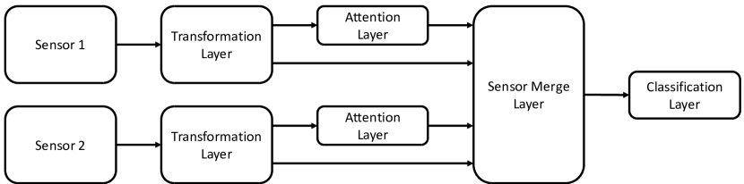
Figure 1: STAN model architecture.

3 Random Walk Noise Training

To enable the network model to be robust against a wide variety of noise types, we introduce the random walk noise model below. The noise model aims to have an approximately uniform coverage of noise level over a range $[0,\sigma_{max})$ and no settle-in time that could introduce a sequence length dependence on the noise. The standard deviation of the noise $\sigma$ for an input sequence of $t$ timesteps can be calculated thusly:

$$\begin{split}\sigma(t)=\phi\left(\underbrace{\sigma_{0}+\sum\nolimits_{i=1}^{t}\operatorname{sgn}(s_{i})n_{i}}_{a},\quad\sigma_{max}\right),\\ \sigma_{0}\sim\mathcal{U}(0,\sigma_{max}/2),\quad s_{i}\sim\mathcal{U}(-1,1)\quad n_{i}\sim\Gamma(k,\theta)\end{split}$$ (3)

with $\sigma_{0}$ drawn uniformly over the range $[0,\sigma_{max}/2)$ and $n_{i}$ drawn from a gamma distribution with shape $k$ and scale $\theta$. The signum function extracts positive and negative signs from $s_{i}$ with equal probability. A parameter search during our experiments yielded $\sigma_{max}=3$, $k=0.8$ and $\theta=0.2$ as an appropriate set of parameters. We define the reflection function $\phi(a,\sigma_{max})$ as

$$\phi(a,\sigma_{max})=\sigma_{max}-\Big{\lvert}\bmod(a,2\sigma_{max})-\sigma_{max}\Big{\rvert}$$ (4)

where $\bmod(a,2\sigma_{max})=a-2\sigma_{max}\lfloor a/2\sigma_{max}\rfloor$ maintains the values within the desired range $(0,2\sigma_{max})$ and the subsequent shift and magnitude operations map the values to the range $[0,\sigma_{max})$ while avoiding discontinuities. Finally the input data $x$ at feature index $k$ and time index $t$ is mixed with the noise sampled from a normal distribution as follows:

$$x_{k,t}=x_{k,t}+n_{k,t},\qquad n_{k,t}\sim\mathcal{N}(0,\sigma^{2}(t))$$ (5)

The reflection function $\phi(a,\sigma_{max})$ performs similarly to the $\bmod$ operator, but at the edges, produces a continuous reflection about the edge instead of a discontinuous wrap. Therefore, this forms a constrained random walk, limited by $\sigma_{max}$, which will become the standard deviation of normally distributed random noise added to the input $x$ at feature index $k$ and time point $t$. This noise model generates sequences that provide a useful training ground to tune the attention mechanism of STAN models, as the noise level varies over time and allows periods of low noise (high attention desired) and high noise (low attention desired). An example for video frames is shown in Figure 2.

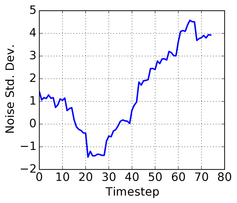
(a)

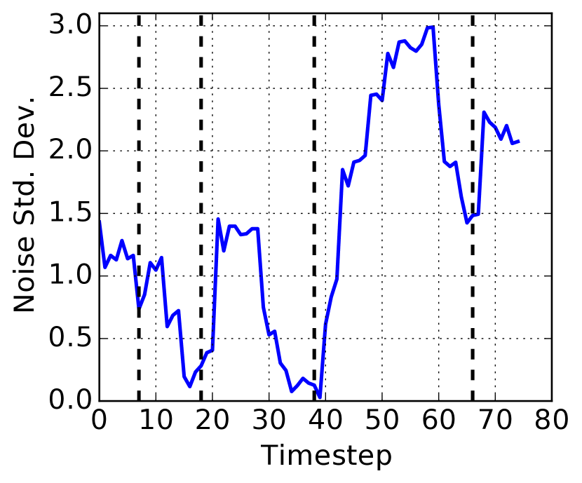
(b)

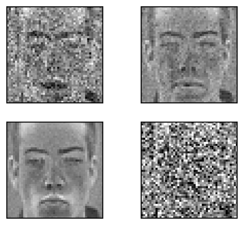
(c)

Figure 2: Depiction of the random walk noise added during training. In (a), the cumulative sum of a sequence of random variables forms a random walk. In (b), the random walk becomes bounded after applying the reflection operator $\phi$ in Eq. 4. On the four sub-panels in (c), a visualization of the noise drawn at each time point. Each panel depicts a video frame from the GRID corpus, zero mean and unit variance normalized, mixed with a Gaussian noise source whose standard deviation corresponds to a vertical dotted line in (b).

4 Experiments

This section presents experiments that show the performance of STANs in environments with dynamically changing noise levels and tested on three commonly-used datasets, namely TIDIGITS, Wall Street Journal and GRID.

4.1 Noise Experiments

Dataset

Table 1: Models used for evaluation on TIDIGITS.

Name	Architecture	Sensors	Transformation Layers	Attention Layers	Classification Layers	Parameters
Single Audio	Baseline	1 Audio	Identity	None	(150,100) GRU	162262
Double Audio STAN	STAN	2 Audio	Identity	(20) GRU	(150,100) GRU	169544
Triple Audio STAN	STAN	3 Audio	Identity	(20) GRU	(150,100) GRU	173185
Double Audio Concat	Concatenation	2 Audio	Identity	None	(150,100) GRU	179812
Triple Audio Concat	Concatenation	3 Audio	Identity	None	(150,100) GRU	197362

The TIDIGITS dataset [15] was used as an initial evaluation task to demonstrate the response of the attentional signal to different levels of noise in multiple sensors. The dataset consists of 11 spoken digits (‘oh’, ‘zero’ and ‘1’ to ‘9’) in sequences of 1 to 7 digits in length, e.g ‘1-3-7’ or ‘5-4-9-9-8’. The dataset is partitioned into a training set of 8623 samples and a test set of 8700 samples. The raw audio data was converted to 39-dimensional Mel-frequency cepstral coefficients [6] features (12 Mel spaced filter banks, energy term, first and second order delta features). A frame size of 25ms and a frame shift of 10ms were applied during feature extraction. The features are zero-mean and unit-variance normalized on the whole dataset. The sequence error rate (SER) is used as a performance metric. It is defined as the number of entirely correct sequence transcriptions $C$ over the number of all sequences $A$: SER [%] = $\frac{C}{A}$.

Models

A total of five models were evaluated, with a summary given in Table 1. The classification stage is the same two-layer unidirectional (150,100) GRU network followed by an affine transform to 12 classes (blank label + vocabulary) for all models. The baseline model consists of a single audio sensor that is directly connected to the classification stage. Two models make use of the STAN architecture with two or three sensors. The attention modules consist of (20) GRUs and their output is converted to one scalar attention score per frame by an affine transform. In order to evaluate the potential benefit of STAN architectures, they are compared against two simpler sensor concatenation models. Those two have either two or three sensors, whose input is concatenated and presented directly to the classification network. In these models, the transformation layers were simply the identity function as the task is sufficiently simple to not require their use. The number of parameters is approximately equal for all models and depends only on the number of input sensors.

Training

The connected digit sequences allow for a sequence-to-sequence mapping task. In order to automatically learn the alignments between speech frames and label sequences, the Connectionist Temporal Classification (CTC) [8] objective was adopted. All models were trained with the ADAM optimizer [12] for a maximum of 100 epochs, with early stopping preventing overfitting. Every model was trained on a noisy training set corrupted by random walk noise as detailed in section 3. Each sensor received a unique, independently drawn noise signal per training sample. The noise level of the random walks varied between $[0,3\sigma]$.

Results

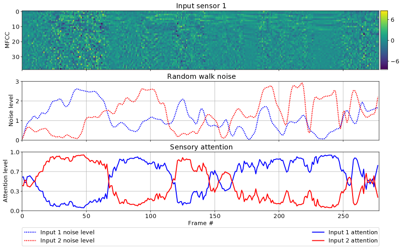
Figure 3: Attention response to random walk noise conditions of a double audio STAN model trained on TIDIGITS. The figure shows the MFCC features with noise of sensor 1 (top), the noise levels applied to both sensors (middle) and the attention values for both sensor (bottom). The STAN model shows the desired negative correlation between noise level and attention for sensors.

Two key results emerge from this initial experiment: first, the attention mechanism generalizes across a variety of noise types; and, secondly, STAN models outperform, in error rate, merely concatenating input feature together. To demonstrate, Figure 3 shows the attention response of a Double Audio STAN model with two audio sensors in response to random walk noise. A sample from the test set was corrupted by random walk with a noise level in the range $[0,3\sigma]$. The model shows the desired negative correlation between noise level and attention: when the noise level for a sensor goes up, the attention paid to the same sensor goes down. As the noise levels interleave over time, the attention mechanism is able to switch between sensors by a delay of 1-5 frames. Furthermore, without additional training, the same model is evaluated against novel noise types in Figure 4. The attention modules successfully focus their attention on the sensor with the lowest noise level under a variety of noise conditions. In situations where the noise level of both sensors is low, such as seen in the noise burst or sinusoidal noise cases, the attention settles in an equilibrium between both sensors.

To determine whether the attention across sensors actually improves performance, the STAN models are evaluated against a baseline single sensor model and concatenation models under both clean and noisy conditions. With the clean testset, all available sensors are presented the same clean signal. With the noisy testset, each sensors data is corrupted by unique random walk noise with a standard deviation in the range $[0,3\sigma]$. The results are reported in Figure 5(a). All models achieve comparably low SER around $3\%$ on the clean test set, despite training on noisy conditions, implying the STAN architecture does not have negative implications for clean signals. On the noisy test set, the STAN models with two and three sensors perform best. The STAN models lower the SER by 66.8% (single vs. double sensors) and 75% (single vs. triple sensors) through additional inputs. The STAN models dramatically outperform the concatenation models with an equivalent number of sensors, achieving around half the SER, suggesting concatenation models had difficulties in prioritizing signal sources with lower noise levels.

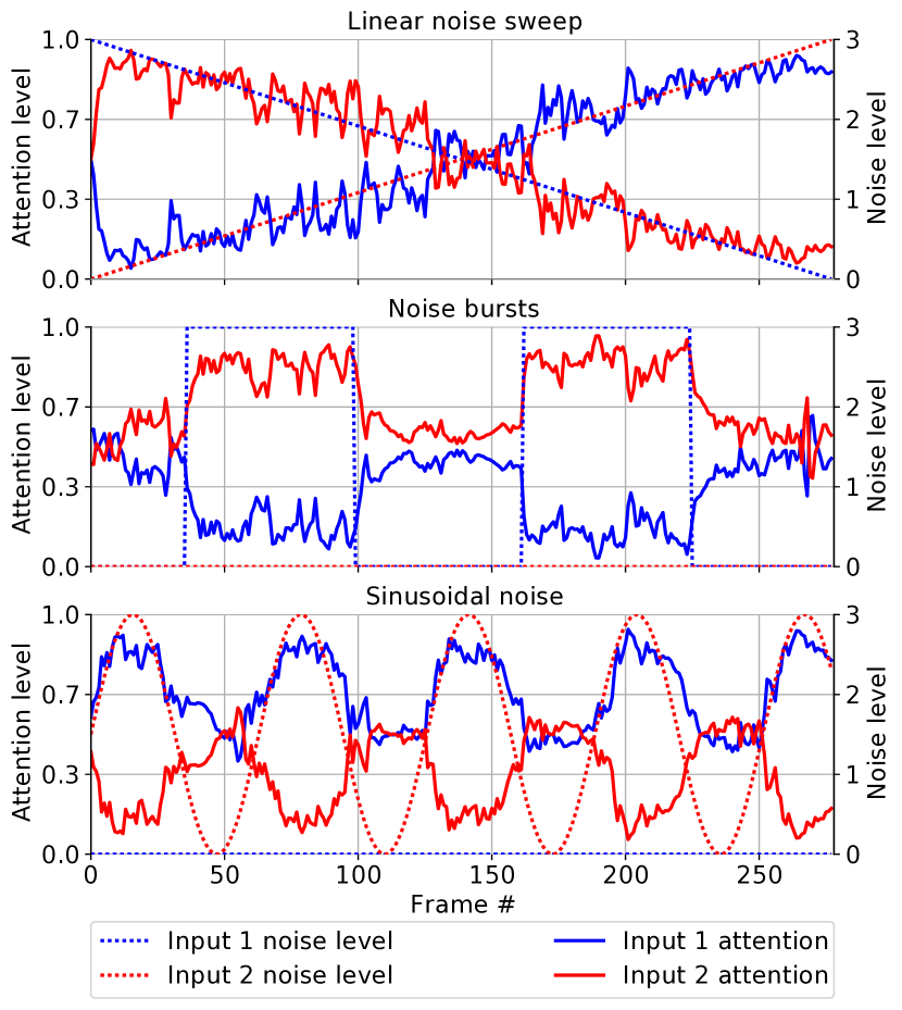
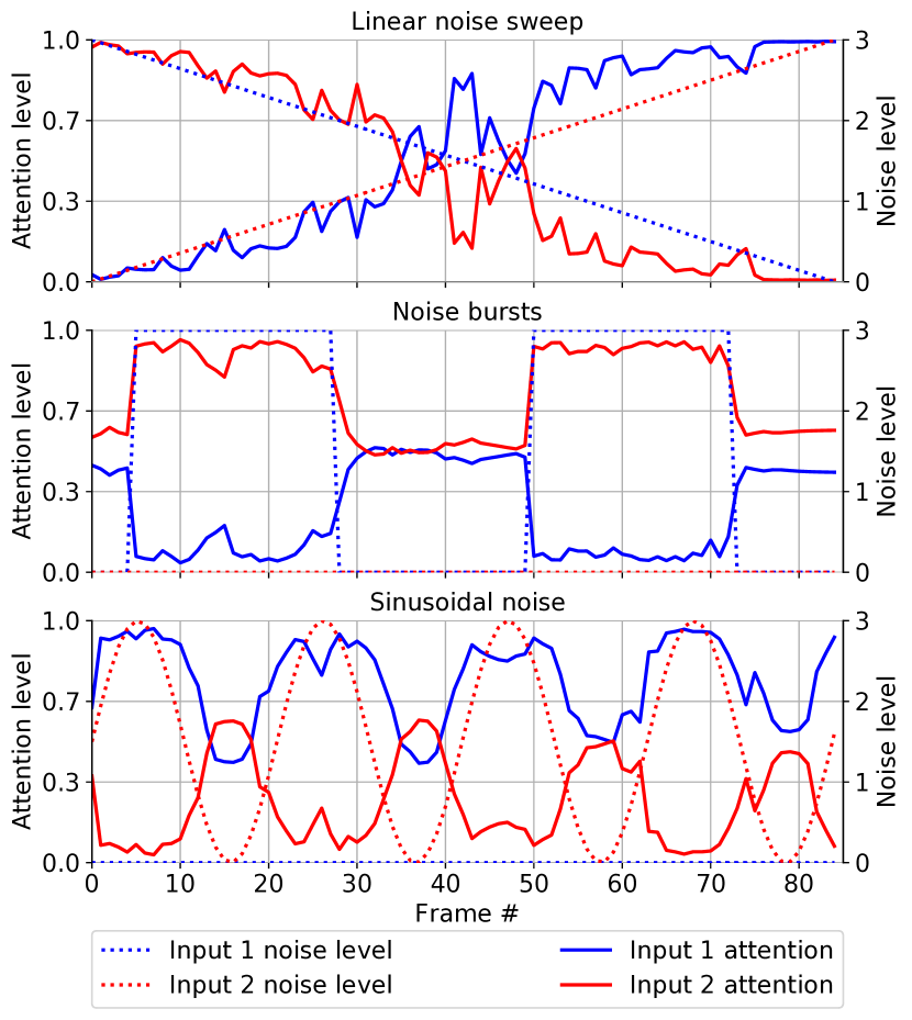
Figure 4: Attention response to various noise conditions of a double sensor STAN model trained on audio (TIDIGITS, left side) and video (GRID, right side). Three noise responses are shown: linear noise sweeps on both sensors (top), noise bursts on sensor 1 (middle) and sinusoidal noise on sensor 2 (bottom). Though these noise conditions were not seen during training, both STAN models show the desired negative correlation between noise level and sensor attention.

4.2 Transfer of Sensor Selection Attention Mechanism to WSJ Corpus

Dataset

This experiment demonstrates the possibility to train a STAN model on a small dataset (TIDIGITS) and transfer the sensor selection attention mechanism to a non-STAN model that was independently trained on a much bigger dataset ( Wall Street Journal (WSJ)). The WSJ database consists of read speech from the Wall Street Journal. Following standard methodology [16], the 81 hour subset ‘si284’ was used as training set (37416 sentences), the subset ‘dev93’ as development set (513 sentences) and the ‘eval92’ (330 sentences) subset was used as test set.

For both datasets, the raw audio data is converted to 123 dimensional filterbank features (40 filterbanks, 1 energy term and first and second order delta features). During feature extraction, the same frame size of 25ms and frame shift of 10ms were used on both datasets, resulting in longer frame sequences on WSJ. The features were generated by pre-processing routines from EESEN [16]. Each feature dimension is zero-mean and unit-variance normalized.

Models

The TIDIGITS-STAN model uses two audio sensors that provide filterbank features, identity transformation layers and 60 GRUs per attention layer followed by an learned outer product transform to a single attention score per frame. The classification stage on top of the sensor merge layer is built of a unidirectional two-layer (150, 100) GRU network followed by an affine transform to 12 classes. The TIDIGITS-STAN model uses 267k parameters, with the classification stage accounting for 200k parameters (75%).

The WSJ-baseline model is a non STAN model that is trained independently and consists of 8.5M parameters. It is built of 4 layers of bidirectional long short-term memorys [9] units with 320 units in each direction, followed by an affine transformation that maps the last layers output to the 59 output labels (blank label + characters). The WSJ-baseline model maps filterbank feature sequences to character sequences. Similar architectures can be found in literature [16]. We build a WSJ-STAN model by the following recipe: first, the TIDIGITS-STAN model is trained. Second, we train the WSJ-baseline model. Third, we replace the classification stage of our TIDIGITS-STAN model with the WSJ-baseline model. The result of this replacement process is the WSJ-STAN model, on which no retraining is performed. The standard performance metric on WSJ is the word error rate (WER), which is defined as following: WER [%] = $\frac{S+D+I}{N}$, with word level substitutions $S$, deletions $D$, insertions $I$ and the number of words in the reference $N$.

Training

Both TIDIGITS and WSJ allow for a sequence-to-sequence mapping task. In order to automatically learn the alignments between speech frames and label sequences, the CTC [8] objective was adopted. The models were trained with the ADAM optimizer [12] for a maximum of 100 epochs, with early stopping preventing overfitting. The TIDIGITS-STAN model was trained on TIDIGITS training set which was corrupted by random walk noise as detailed in section 3. Each sensor received a unique, independently drawn noise signal per training sample again in the range $[0,3\sigma]$. The WSJ-baseline model was trained on the WSJ ‘train-si84’ training set, which contained clean speech only.

Results

The WSJ-baseline model and the WSJ-STAN model are evaluated on the ‘eval92’ test set from the WSJ corpus. In Table 2 we report the WER after decoding the network output with a trigram language model based on Weighted Finite State Transducers [17], see [16] for details. For the clean speech test, the same clean signal is used as input for both sensors of the WSJ-STAN model, it should thus be equivalent to the baseline model in the clean test case. This is confirmed as the both the WSJ-baseline and the WSJ-STAN models achieve the same 8.4% WER on clean speech, which is close to state-of-the art with comparable setups [16]. In the noisy tests, the input features are overlaid with random walk noise with a noise level of up to $3\sigma$. There, the WSJ-STAN model achieves 26.1% WER, while the WSJ-baseline model has over double the error rate at 53.5% WER. This result demonstrates clearly that the STAN architecture can generalize its sensor selection attention mechanism to different datasets and different classification stages. It is notable that even though the average number of frames per sample in the WSJ ‘eval92’ test set (760) is approximately 4.6X larger than that of the TIDIGITS test set (175), the attention mechanism still functions well.

Table 2: Evaluation results on the WSJ corpus: WER in [%] after decoding

Model	WSJ-baseline	WSJ-STAN
Clean test set	8.4	8.4
Noisy test set	53.5	26.1

4.3 Correct Fusion from Multiple Sensors on Grid

Dataset

The GRID [5] corpus is used for perceptual studies of speech processing. There are 1000 sentences spoken by each of the 34 speakers. The GRID word vocabulary contains four commands (‘bin’, ‘lay’, ‘place’, ‘set’), four colors (‘blue’, ‘green’, ‘red’, ‘white’), four prepositions (‘at’, ‘by’, ‘in’, ‘with’), 25 letters (‘A’-‘Z’ except ‘W’), ten digits (‘0’-‘9’) and four adverbs (‘again’, ‘now’, ‘please’, ‘soon’), resulting in 51 classes. There are 24339 training samples and 2661 test samples, consisting of both audio and video data. The raw audio data was converted to 39-dimensional MFCCs features (12 Mel spaced filter banks, energy term, first and second order delta features). During feature extraction, a frame size of 60ms and a frame shift of 40ms were applied to match the frame rate. The video frames are converted to grey level frames. Both audio and video data are normalized to zero-mean and unit-variance on the whole dataset. As for TIDIGITS, the SER is used as a performance metric.

Training

The video and audio sequences of the GRID database allow for a sequence-to-sequence mapping task. In order to automatically learn the alignments between speech frames, video frames and label sequences, the CTC [8] objective was adopted. The output labels consisted of 52 classes (vocabulary size + blank label). All models were trained with the ADAM optimizer [12] for a maximum of 100 epochs, with early stopping preventing overfitting. Every model was trained on a noisy training set corrupted by random walk noise as detailed in section 3. Each sensor received a unique, independently drawn noise signal per training sample. The noise level of the random walks varied in the range $[0,3\sigma]$.

Table 3: Models used for evaluation on GRID.

Name	Architecture	Sensors	Transformation Layers	Attention Layers	Classification Layers	Parameters
Single Audio	Baseline	1 Audio	(50) Dense	None	(200,200) BI-GRU	1030012
Double Audio STAN	STAN	2 Audio	(50) Dense	(20) GRU	(200,200) BI-GRU	1056654
Triple Audio STAN	STAN	3 Audio	(50) Dense	(20) GRU	(200,200) BI-GRU	1062955
Double Audio Concat	Concatenation	2 Audio	(50) Dense	None	(200,200) BI-GRU	1108052
Triple Audio Concat	Concatenation	3 Audio	(50) Dense	None	(200,200) BI-GRU	1170052
Single Video	Baseline	1 Video	CNN	None	(200,200) BI-GRU	1061126
Double Video STAN	STAN	2 Video	CNN	(150) GRU	(200,200) BI-GRU	1087562

Models

A total of seven models were evaluated: five models that use audio input only and two model that use video input only. A summary is given in Table 3. All models use a two-layer bidirectional GRU network with (200, 200) units in each direction followed by an affine transform to 52 classes (blank label + vocabulary) for the classification stage. The audio-only models consist of a baseline single sensor model, two STAN models with either two or three sensors and two concatenation models with two or three sensors. Every audio sensor makes use of a (50) unit non-flattening dense layer with a $tanh$ non linearity for feature transformation. For the STAN models, the attention layers operate on the transformed features and use 20 GRUs per sensor. Their output is converted to one scalar attention score per frame by an affine transform. The video-only models use a CNN for feature transformation: three convolutional layers of 5x5x8 (5x5 filter size, 8 features), each followed by a 2x2 max pooling layer. The output is flattened and presented to classification layer. The double video STAN model uses attention layers with 150 GRUs per sensor.

Results

The seven previously described models are compared by their SER on the GRID test set. The testing is carried out on a clean variant and a noise corrupted variant of the test set. With the clean test set, all sensors of the same modality are presented with the same clean signal. With the noisy test set, each sensor’s data is corrupted by unique random walk noise with a noise level in the range $[0,3\sigma]$. The results are reported in Figure 5(b). All of the audio-only models achieve comparably low SER around $5\%$ on the clean test set, even though they were trained on noisy conditions, echoing the results found for TIDIGITS. On the noisy test set, the audio STAN models are able to outperform their concatenation counterparts by 13% (two sensors) and 17% (three sensors). Adding more sensors to the STAN models relatively lowers the SER by 48% (single vs. double audio sensors) and 58% (single vs. triple audio sensors).

The video-only baseline model achieves a performs worse than the single audio-only model on both clean and noisy test conditions. However, the STAN model is still able to improve the SER scores. The sensor selection attention mechanism also works on video data, as depicted in Figure 4. In order to successfully train the STAN model for video data, the attentional and transformation layer weights are shared across both sensors.

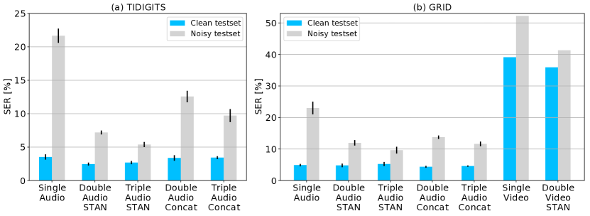
Figure 5: SER scores on (a) TIDIGITS and (b) GRID datasets for clean and noisy testsets. The audio scores represent the mean of 5 weight initializations, while the video scores are based on a single weight initialization. The SER is a tough error measure that penalizes the slightest error in a sequence transcription. Our GRID video models achieve a 90.5% (Single Video) and 91.5% (Double Video STAN) label-wise accuracy on clean video. These results compare with state-of-the-art [1] without data augmentation or architecture specialization.

5 Discussion

The Sensor Transformation Attention Network architecture has a number of interesting advantages that merit further analysis. By equipping each sensory modality with a mechanism for distinguishing meaningful features of interest, networks can learn how to select, transform, and interpret their sensory stimuli. First, and by design, STANs exhibit remarkable robustness to noise sources. By challenging these networks during training with dynamic and persistent noise sources, the networks learn to rapidly isolate modalities corrupted by noise sources. We further show that this results in even better performance than maintaining the full high-dimensional space created by concatenating all inputs together. The sensor selection attention mechanism shows remarkable generalization properties: we demonstrated that it can be trained on a small dataset and be reused on a much bigger dataset that demands a much more powerful classification stage.

This architecture also permits investigation of common latent representations reused between sensors and modalities. Similar to the “interlingua” mentioned in machine translation work [18], perhaps the transformation layer allows sensors to map their inputs to a common, fused semantic space that simplifies classification. As has been pointed out in a variety of other studies, attention is a powerful mechanism to aid in network interpretability [19]. Here, attention is used to select among sensors, but this could easily be extended to e.g., foveated representations of the environment, allowing very precise analysis of determining the causality of neural network decisions. Future work could also investigate the inherent informativeness of the attentional signal itself to determine e.g., the direction of approach of an ambulance in a multi-audio setup.

References

- [1] Y. M. Assael, B. Shillingford, S. Whiteson, and N. de Freitas. Lipnet: Sentence-level lipreading. arXiv preprint arXiv:1611.01599, 2016.
- [2] D. Bahdanau, K. Cho, and Y. Bengio. Neural machine translation by jointly learning to align and translate. arXiv preprint arXiv:1409.0473, 2014.
- [3] D. Bahdanau, J. Chorowski, D. Serdyuk, P. Brakel, and Y. Bengio. End-to-end attention-based large vocabulary speech recognition. In 2016 IEEE International Conference on Acoustics, Speech and Signal Processing (ICASSP), pages 4945–4949, 2016.
- [4] J. Chung, C. Gulcehre, K. Cho, and Y. Bengio. Empirical evaluation of gated recurrent neural networks on sequence modeling. arXiv preprint arXiv:1412.3555, 2014.
- [5] M. Cooke, J. Barker, S. Cunningham, and X. Shao. An audio-visual corpus for speech perception and automatic speech recognition. The Journal of the Acoustical Society of America, 120(5):2421–2424, 2006.
- [6] S. Davis and P. Mermelstein. Comparison of parametric representations for monosyllabic word recognition in continuously spoken sentences. IEEE transactions on acoustics, speech, and signal processing, 28(4):357–366, 1980.
- [7] R. Desimone and J. Duncan. Neural mechanisms of selective visual attention. Annual review of neuroscience, 18(1):193–222, 1995.
- [8] A. Graves, S. Fernández, F. Gomez, and J. Schmidhuber. Connectionist temporal classification: labelling unsegmented sequence data with recurrent neural networks. In Proceedings of the 23rd International Conference on Machine learning, pages 369–376. ACM, 2006.
- [9] S. Hochreiter and J. Schmidhuber. Long short-term memory. Neural Computation, 9(8):1735–1780, 1997.
- [10] C. Hori, T. Hori, T.-Y. Lee, K. Sumi, J. R. Hershey, and T. K. Marks. Attention-based multimodal fusion for video description. arXiv preprint arXiv:1701.03126, 2017.
- [11] S. Kim and I. Lane. Recurrent models for auditory attention in multi-microphone distant speech recognition. Interspeech 2016, pages 3838–3842, 2016.
- [12] D. Kingma and J. Ba. Adam: A method for stochastic optimization. arXiv preprint arXiv:1412.6980, 2014.
- [13] A. Krizhevsky, I. Sutskever, and G. E. Hinton. Imagenet classification with deep convolutional neural networks. In Proc. of NIPS, pages 1097–1105, 2012.
- [14] Y. LeCun, L. Bottou, Y. Bengio, and P. Haffner. Gradient-based learning applied to document recognition. Proceedings of the IEEE, 86(11):2278–2324, 1998.
- [15] R. G. Leonard and G. Doddington. TIDIGITS speech corpus. Texas Instruments, Inc, 1993.
- [16] Y. Miao, M. Gowayyed, and F. Metze. EESEN: End-to-end speech recognition using deep RNN models and WFST-based decoding. In 2015 IEEE Workshop on Automatic Speech Recognition and Understanding (ASRU), pages 167–174, 2015.
- [17] M. Mohri, F. Pereira, and M. Riley. Speech recognition with weighted finite-state transducers. In Springer Handbook of Speech Processing, pages 559–584. Springer, 2008.
- [18] Y. Wu, M. Schuster, Z. Chen, Q. V. Le, M. Norouzi, W. Macherey, M. Krikun, Y. Cao, Q. Gao, K. Macherey, et al. Google’s neural machine translation system: Bridging the gap between human and machine translation. arXiv preprint arXiv:1609.08144, 2016.
- [19] K. Xu, J. Ba, R. Kiros, K. Cho, A. Courville, R. Salakhutdinov, R. Zemel, and Y. Bengio. Show, attend and tell: Neural image caption generation with visual attention. In Proc. of the 32nd International Conference on Machine Learning, volume 37, 2015.