Stability for implicit-explicit schemes for non-equilibrium kinetic systems
in weighted spaces with symmetrization

Abstract

We consider kinetic systems, and prove their stability working in weighted spaces in which the systems are symmetric. We prove stability for various explicit and implicit semi-discrete and fully discrete schemes. The applications include advective and diffusive transport coupled to the accumulation of immobile components governed by non-equilibrium relationships. We also discuss extensions to nonlinear relationships and multiple species.

Keyword: stability for systems, kinetic models, non-equilibrium, adsorption, symmetrization, implicit schemes, explicit schemes

1 Introduction

In this paper we transform and analyze semi-implicit numerical schemes for an evolution system

$$(\phi u)_{t}+v_{t}+\nabla\cdot(qu)-\nabla\cdot(\phi d\nabla u)=f,$$ (1a)

$$v_{t}=\alpha(g(u)-v)$$ (1b)

which arises in a variety of important applications, e.g., transport in porous media with adsorption. Here $\alpha>0$ and $g(\cdot)$ is monotone, with details below. The positive coefficient $\phi$ is the porosity.

For this system there is no maximum principle, and if $f=0$, there is not even a natural conservation or stability principle in the natural norms of $(u,v)$. Further, the analysis of the simple finite discretization schemes with well known truncation errors, even when $g$ is linear, has to deal with nonnormality, and is unnecessarily complex, even when $g(\cdot)$ is linear.

The transformation we propose involves symmetrization, rescaling, and a change of variables. Equivalently, we work in weighted spaces. We exploit the symmetrization to prove strong stability of the problem and of the associated numerical schemes, from which the natural error estimates follow. For fully implicit schemes the framework of m-accretive operators reduces the stability analysis to the verification that the operator is m-accretive. However, for implicit-explicit schemes this is not sufficient, and we draw upon Fourier analysis.

Overview

For the linear case when $g(u)=cu$, with $c>0$, the abstract form of (1) has the structure of a linear kinetic system

$$U^{\prime}+V^{\prime}+LU = F$$ (2a)

$$V^{\prime}+\alpha(V-cU) = 0,$$ (2b)

with the unknowns $U,V:(0,T]\to H\times H$, where $H$ is an appropriate Hilbert space to be defined, and the source term$F:[0,\infty)\in H$ is given. The linear transport operator $L$ is defined in the sequel, and we will require for $L$ to be m-accretive to get strong stability.

Our main technical objective is to study the stability of (2) and of one–step implicit and implicit-explicit discrete schemes for (2)

$$\frac{U^{n}-U^{n-1}}{\tau}+\frac{V^{n}-V^{n-1}}{\tau}+LU^{n*} = F^{n}$$ (3a)

$$\frac{V^{n}-V^{n-1}}{\tau}+\alpha(V^{n}-cU^{n}) = 0.$$ (3b)

which is solved at every time step $n=1,2,\ldots$ for the approximations $U^{n},V^{n}$ to $u(\cdot,t_{n}),v(\cdot,t_{n})$. Here $F^{n}\approx F(t_{n})$. This one-step scheme is fully implicit if $n*=n$. Other schemes arise for $n*\neq n$. The analysis of (3) involves consideration of spatial discretization as well as of time discretization. Our technique of symmetrization allows to demonstrate strong stability of the schemes in a weighted space, even though the original system (2) has nonnormal operators.

Extensions of (2) to nonlinear systems and to systems with multiple components will be also discussed.

Motivation and context

The problem (1) comes from applications in subsurface modeling such as the transport of contaminant undergoing adsorption, or coalbed methane reservoir simulation, but cover also a variety of other applications. In those problems (1) represents the conservation of mass of some chemical component, with $u$ denoting the mobile concentration, and $v$ representing the immobile component, while $g(\cdot)$ a general monotone (increasing) function. We provide details on the applications in Section 2.

Numerical analysis of (1) with non-equilibrium kinetics was given in [1] for diffusion only, with focus on non-Lipschitz $g(\cdot)$ important for liquid adsorption. In [2] Lagrangian techniques for advection with non-equilibrium adsorption and in [3] the Lagrangian transport combined with Galerkin approximation to diffusion were analyzed. In addition, in a sequence of papers devoted to the scalar conservation laws with relaxation terms [4] a problem similar to (4a) but without diffusion is studied, and convergence order of $O(\sqrt{h})$ is established. In turn, in [5] we studied the stability of schemes for a single equation analogue of (4a) without diffusion and where $v$ was eliminated, and in [6] we extended the analysis to cover the linear case with diffusion. Furthermore, previous results on stability of schemes of (2) for the case of initial equilibrium were shown in [7, 5, 6].

Our approach in this paper provides a unified framework for the analysis of a variety of explicit and implicit finite difference schemes for the non-equilibrium advection-diffusion problems. In particular, it establishes strong stability as well as optimal error estimates of order $O(h)$ or $O(h^{2})$.

Outline

In Section 2 we motivate the study of (2), provide examples of $L$, and provide literature review. In Section 3 we describe the main idea of symmetrization in the abstract setting leading to the stability of the numerical schemes. In Section 4 we provide concrete examples of fully discrete schemes for (2) and evaluate their stability, and in Section 5 we illustrate the theory with numerical examples, and convergence studies. We close in Section 6, where we outline extensions to the nonlinear and multi-species case, and discuss future work.

Notation and assumptions

Throughout the paper we assume that $c>0,\alpha>0$; otherwise, the system is decoupled and trivial. $I$ always denotes the identity operator or matrix, as is clear from the content.

With the original variables in (1) denoted by $u(x,t)$ and $v(x,t)$, we consider the vectors $U(t)=u(\cdot,t)=\left(u(x,t)\right)_{x}\in H$. Each $U(t),V(t)$ lives in a Hilbert space $H$, with the inner product denoted by $\langle\cdot,\cdot\rangle_{H}$; we drop the subscript $H$ when it does not lead to a confusion. The domain of an operator $L$ is denoted by $D(L)$, and the time derivative $U^{\prime}(t)$ or $\frac{dU}{dt}(t)$ generalizes the partial derivative $\frac{\partial}{\partial t}$, and is defined in an appropriate abstract setting, such as that developed in [8].

The vector $W=W(t)=[U(t),V(t)]^{T}$ lives in $H\times H$, which is endowed either with the natural or weighted inner product, with details below. We also consider new variables $\tilde{W}$ in appropriate spaces. The (matrices of) operators on $W$ or $\tilde{W}$ in the product space $H\times H$ are denoted similarly to those on $H$. In particular, for $L:D(L)\subset H\to H$ we define $\mathcal{L}=\left[\begin{array}[]{cc}L&0\\ 0&0\end{array}\right]$ on $D(\mathcal{L})=D(L)\times H\subset H\times H$. We define $\mathcal{A}$, $\mathcal{D}$ analogously.

In discrete schemes, we consider uniform time stepping $t_{n}=n\tau$ with $n=0,1,\ldots$, and time step $\tau$. For fully discrete schemes, we denote the spatial grid parameter by $h$ and consider finite dimensional analogues of the operators such as $L_{h}$ for $L$. For the unknown $u(x,t)$ we denote by $u^{n}(x)\approx u(x,t_{n})$ its semi-discrete in time approximation, by $U^{n}\in H$ the collection $(u^{n}(x))_{x}\in H$. In turn, $U_{h}(t)=(u_{j}(t))_{j}\in H_{h}$ where $u_{j}(t)\approx u(x_{j},t)$ is the semi-discrete in space approximation, in a discrete (usually finite dimensional) subspace $H_{h}\subsetneq H$ of dimension dependent on $h$. Finally, fully discrete approximations $U_{h}^{n}\approx U_{h}(t_{n})$. Most of our results are formulated on $H$, and are shown to apply on $H_{h}$.

2 Motivation and literature review

In this section we develop the applications which motivate (2) and provide details on its abstract setup, in particular on the properties of $L$ as they follow for the special cases of (1) under assumed boundary conditions. Our presentation of the model follows the literature on coalbed methane adsorption [9, 10, 11] where (1) arises directly, and finite volumes are used; see also our expository work in [12]. In Section 2.3 we discuss a particular direction in which (2) is reduced to a single equation; this is discussed in [5] under initial equilibrium assumption.

2.1 Applications

In porous media, the model of transport with adsorption (1) describes the evolution of the concentration of a chemical. Consider an open bounded region of flow $\Omega\in\mathbf{R}^{k},k=1,2,3$, in which the volumetric flux $q$, with $\nabla\cdot q=0$, is given; assume also the porosity $\phi(x)>0$ and the (uniformly positive definite) diffusion coefficient $d$ are known. If the chemical is adsorbed in the porous medium, the mass conservation must include also the rate of change of the adsorbed immobile amount denoted by $v$. The mass conservation of the chemical being transported by advection $Au=\nabla\cdot(qu)$ and diffusion–dispersoon $Du=-\nabla\cdot(d\nabla u)$ , with adsorption term, is

$$(\phi u)_{t}+v_{t}+Au+Du=f,\;\;\;x\in\Omega,\;\ t>0$$ (4a)

and it remains to specify the relation of $$v u$$ to .

The equilibrium relationship $v=g(u)$ which can be used to complete (4a) assumes that the time scale of transport is much slower than that of the adsorption. In turn, the non-equilibrium or kinetic model

$$v_{t}+\alpha(v-g(u))=0$$ (4b)

allows to treat the time scales of adsorption and of transport on par with each other, with $\alpha>0$ denoting the rate of the process. As $\alpha\to\infty$, it is expected that (4b) has solutions close to the equilibrium. The linear relationship $g(u)=cu$, with $c>0$ is what is assumed throughout most of this paper.

For well-posedness, we require appropriate boundary conditions on $u$ as well as initial conditions for both $u$ and $v$.

2.1.1 Abstract setting

In the abstract form, the model (4a) and (4b), upon absorbing nonessential constants in the definitions of $u$, are written as (2), in which $L=D+A$ is the abstract diffusion-advection transport operator, and where (2) is posed as a Cauchy problem in an appropriate function space.

Consider $L:D(L)\to H$ in a Hilbert space $H$, with domain $D(L)$. We recall that $L$ is accretive if $\langle LU,U\rangle\geq 0$ for any $U\in D(L)$. Additionally, $L$ is m-accretive if $I+L$ is onto $H$ that is, for any $F\in H$ the problem $U+LU=F$ is solvable (from accretiveness there follows the uniqueness of the solution).

For an m-accretive $L$, the following results are well known; see, e.g., [8], (Sec.I.4). The dynamics of $U^{\prime}(t)+LU=0,U(0)\in H$ is governed by a linear contraction semigroup, so that, in particular, $U(t)\in D(L)$. If $L$ is self-adjoint, additional regularity and convergence properties follow. The nonhomomogeneous case of $U^{\prime}(t)+LU=F$ requires that $F\in(C^{1}[0,\infty),H)$. See, e.g. [8], (Prop.4.1) and [13], (Cor. 3.B).

For the applications of (1) described in Sec. 2.1 we consider $H=L^{2}(\Omega)$ with the inner product $\langle\psi,\xi\rangle=\int_{\Omega}\psi\xi$. In the case of periodic boundary conditions, without loss of generality, one can use $\Omega=(0,1)^{k}$, but we only analyze $k=1$ case. We will recall the standard abstract results for $Au=-d\nabla^{2}u+\nabla\cdot(qu)$, with weak rather than the classical (partial) derivatives. The definition of $L$ and $D(L)$ accounts for the boundary conditions. For details on this abstract setup see [13], (Ex. IV.2., p108) and [8], (Prop. I. 4.2, p21). For periodic case, see [13], (Ex IV.1, p107)), and for advection see [13], (Example IV.1).

Remark 1

(i) Let $L=D$, with $d>0$, and with homogeneous Dirichlet boundary conditions imposed. We have $D(L)=H_{0}^{1}(\Omega)\cap H^{2}(\Omega)$, and $L$ is m-accretive self-adjoint. (ii) As in (i), but with homogenous Neumann conditions, $D(L)=H^{2}(\Omega)$, $L$ is m-accretive, and self-adjoint. (iii) As in (i), with periodic boundary conditions, e.g.. when $\Omega=(0,1)$ we have $D(L)=\{\psi\in H^{2}(\Omega),\psi(0)=\psi(1),\psi^{\prime}(0)=\psi^{\prime}(1)\}$. The operator $L$ is m-accretive and self-adjoint. (iv) Case $L=A$, with properly posed conditions on the inflow boundary, or with periodic boundary conditions, e.g., for $\Omega=(0,1)$, $D(L)=\{\psi\in H^{1}(\Omega):\psi(0)=\psi(1)\}$; The operator $D$ is m-accretive but not selfadjoint. (v) Case $L=A+D$, and $d>0$, $q\neq 0$. With periodic b.c., $D(L)$ is as in (iii), and $L$ is m-accretive but not selfadjoint.

2.2 Related models and previous work

In models of transport with gas adsorption, (4b) allows to account for subscale diffusion accompanying the overall transport; see [14, 15]. More general models in which $\alpha$ is a monotone operator can be used, e.g., to model hysteresis in adsorption [16] or non-equilibrium phase transitions [17]. Further, non-equilibrium relation (4b) is used to model transport in media with multiscale character, such as in the classical Warren-Root and Barenblatt models of double porosity [18, 19]; see also modeling and analysis in [20, 21, 22], and numerical analysis in [7, 23].

In previous work for nonlinear $g(\cdot)$ [3] proved a-priori error estimates for Lagrangian-Galerkin methods for (1), and in [1] the analysis is for diffusion only. Our paper handles the advection and diffusion problem together for linear $g(\cdot)$, and handles the analysis as well as implicit and explicit numerical schemes in the same framework.

2.3 Nonlocal formulation in $u$ under the initial equilibrium assumption

One can reformulate the coupled kinetic system (2a) as a single equation with nonlocal in time terms. Recall Volterra convolution integral term defined by $\beta\ast U=\int_{0}^{t}\beta(t-s)U(s)ds$. We solve (2b) for $V(t)$ in terms of $U(t)$ and substitute to (2a) to give the following Volterra integro-differential equation

$$U^{\prime}+\alpha U^{\prime}\ast\beta+AU=F+\beta(t)(V(0)-cU(0)),$$ (5a)

solved for $$U \beta(t)=\alpha e^{-\alpha t} V U$$, where . The variable can be recovered from by

$$V(t)=e^{-\alpha t}V(0)+\int_{0}^{t}\alpha cU(s)e^{-\alpha(t-s)}ds.$$ (5b)

Now we see that the second term on the right hand side of (5a) acts like a source/sink term decreasing with $t$, and it vanishes under the assumption of initial equilibrium

$$V(0)-cU(0)=0.$$ (6)

The one-way coupling in (5) focuses the attention on $U$ while keeping track of the memory effects expressed by $U^{\prime}\ast\beta$.

The effect of memory terms isolated from the source term can be studied if (6) is assumed. This approach was followed in [7, 5, 6]. Strong stability of $u$ for the numerical schemes was proven for $L=D$ in [7], and for linear or nonlinear advection operator $L=A$ in [5], where we exploited the positivity of the kernel $\beta$. Even though we did not prove it, the numerical results suggested that a maximum principle holds for $U$.

If (6) cannot be assumed, the positive source term in (5a) can be expected to disturb the maximum principle and/or stability. Indeed, a simple example in Sec. 5.1 readily demonstrates it.

As concerns numerical schemes, in [7] the kernel was also allowed to be weakly singular, e.g., $\beta=O(t^{-1/2})$, which corresponds to subscale diffusion, i.e., the case when there is diffusion in (2b). A more general case of nonlocal terms and of operators $L$ was studied in [6] in which the multiscale model derived in [24], but initial data was assumed in equilibrium. In [5] we conjectured experimentally that the presence of the memory term $u^{\prime}\ast\beta$ would lead to an increased regularity of the solution $u$ when $\beta$ was weakly singular, but this effect appears weaker for the bounded $\beta$.

Beyond porous media, the effect of non-equilibrum (relaxation) such as in (4b), was studied, e.g., in [25], and is an important component of pseudo-parabolic models [26].

3 Stability for the abstract symmetrized evolution system

We start by motivating the symmetrization and discussing the properties and well-posedness of the symmetrized system in the abstract form on some general Hilbert spaces $H$.

First we re-arrange (2) in an equivalent form

$$U^{\prime}-\alpha(V-cU)+LU = F,$$ (7a)

$$V^{\prime}+\alpha(V-cU) = 0.$$ (7b)

This arrangement is similar to those used in multiscale models such as the Warren-Root or Barenblatt models [18, 19]. For these models however $c=1$; their analysis and numerics can be found, e.g., in [23]. When $c\neq 1$, the analysis requires additional work.

In a vector-matrix form with $w=[u,v]^{T}$ we write (7)

$$W^{\prime}+\mathcal{B}W=W^{\prime}+\mathcal{C}W+\mathcal{L}W=[F,0]^{T},$$ (8)

with

$$\mathcal{C}=\alpha\left[\begin{array}[]{cc}cI&-I\\ -cI&I\end{array}\right],\;\;\mathcal{L}=\left[\begin{array}[]{cc}L&0\\ 0&0\end{array}\right].$$ (13)

This system of evolution equations is solved for $W(t)=[U(t),V(t)]^{T}\in H\times H$. The space $H\times H$ is endowed with the natural inner product $(\cdot,\cdot)_{H\times H}$ and norm ${\parallel\!\cdot\!\parallel}_{H\times H}$ on the product space, where $\langle[U,V]^{T},[\phi,\psi]^{T}\rangle_{W}=\langle U,\phi\rangle_{H}+\langle V,\psi\rangle_{H}$.

Challenge

The system (8) is linear, and thus is trivially well-posed, e.g., if $H=\mathbf{R}^{P}$, $P\in\mathbb{N}$. However, in Section 5.1 we show with a simple example on $H=\mathbf{R}$, that the system (8) is not stable in ${\parallel\!w\!\parallel}_{H\times H}$, even though the solutions to the homogeneous problem eventually decay to $0$.

Unless $c=1$, the operator $\mathcal{C}$ and $\mathcal{B}$ are not self-adjoint and nonnormal with respect to $\langle\cdot,\cdot\rangle_{H\times H}$. In consequence, the analysis of the numerical schemes for (8) is quite complicated. Therefore, we consider a weighted inner product on $H\times H$ or, equivalently, a change of variables. This idea which we explain in Sections 3.1 and 3.3, makes the subsequent analysis of numerical schemes fairly straightforward.

3.1 Symmetrization and rescaling

We propose to consider a weighted (scaled) inner product $\langle\cdot,\cdot\rangle_{H}$ on $H\times H$, and an associated norm ${\parallel\!\cdot\!\parallel}_{c}$

$$\langle[U,V]^{T},[\phi,\psi]^{T}\rangle_{c}=c\langle U,\phi\rangle_{H}+\langle V,\psi\rangle_{H},\;\;{\parallel\![U,V]^{T}\!\parallel}_{c}^{2}=c{\parallel\!U\!\parallel}^{2}_{H}+{\parallel\!V\!\parallel}_{H}^{2}.$$ (14)

In other words, instead of $H\times H$ we consider the new (Hilbert) space $W_{c}$ which is $H\times H$ endowed with $\langle\cdot,\cdot\rangle_{c}$. In the new space $W_{c}$ we are able to prove the stability of the evolution system, and of the appropriate numerical schemes for the diffusion-advection examples.

The use of weighted inner product space can be interpreted as changing variables from $U$ to $\tilde{U}=\sqrt{c}U$, since ${\parallel\![U,V]^{T}\!\parallel}_{c}^{2}={\parallel\![\sqrt{c}U,V]^{T}\!\parallel}_{H\times H}^{2}$. We also denote the change of variables from $w$ to $\tilde{w}$ with

$$\tilde{W}=[\tilde{U},V]^{T}=[\sqrt{c}U,V]^{T}.$$ (15)

To show how we exploit the space $W_{c}$, we rewrite (7) by scaling the first component equation of (7) by $\sqrt{c}$, and re-distributing the appropriate constants, by linearity of $L$. We see that (7) is equivalent to

$$\sqrt{c}U^{\prime}-\alpha(\sqrt{c}V-c\sqrt{c}U)+L\sqrt{c}U = \sqrt{c}F$$ (16a)

$$V^{\prime}+\alpha(V-\sqrt{c}\sqrt{c}U) = 0.$$ (16b)

where we have also used $cU=\sqrt{c}\sqrt{c}U$ in (16b). Rewriting in the new variables

$$\tilde{W}^{\prime}+\tilde{\mathcal{B}}\tilde{W}=\tilde{W}^{\prime}+\tilde{\mathcal{C}}\tilde{W}+\mathcal{L}\tilde{W}=[\tilde{F},0]^{T}$$ (17)

with $\tilde{F}=\sqrt{c}F$ and the operators defined as

$$\tilde{\mathcal{B}}=\tilde{\mathcal{C}}+\mathcal{L},\;\;\tilde{\mathcal{C}}=\alpha\left[\begin{array}[]{c c}cI&-\sqrt{c}I\\ -\sqrt{c}I&I\end{array}\right].$$ (20)

3.2 Well-posedness

Now we complete the formal discussion of the well-posedness of (8). We see that $B:D(B)\to H\times H$ with $D(B)=D(L)\times H$ is dense in $H\times H$. Similarly, $\tilde{\mathcal{B}}:D(\tilde{\mathcal{B}})\to W_{c}$, and simply $D(\tilde{\mathcal{B}})=D(B)=D(L)\times H$.

Proposition 1

Let $L$ be m-accretive on $H$. Then the operator $B$ is m-accretive on $W_{c}$. Equivalently, $\tilde{\mathcal{B}}$ is m-accretive on $H\times H$.

Proof: (i) The proof follows from (20) and (15) by the calculation

$$\langle\tilde{\mathcal{B}}\tilde{W},\tilde{W}\rangle_{H\times H}\\ =\langle[(L+c\alpha I)\tilde{U}-\alpha\sqrt{c}IV,-\alpha\sqrt{c}I\tilde{U}+\alpha IV]^{T},[\tilde{U},V]^{T}\rangle_{H\times H}\\ =\langle L\tilde{U}+c\alpha\tilde{U}-\alpha\sqrt{c}V,\tilde{U}\rangle_{H}+\langle-\alpha\sqrt{c}\tilde{U}+\alpha V,V\rangle_{H}\\ =\langle L\tilde{U},\tilde{U}\rangle_{H}+c\alpha\langle\tilde{U},\tilde{U}\rangle_{H}-2\alpha\sqrt{c}\langle V,\tilde{U}\rangle_{H}+\alpha\langle V,V\rangle_{H}=\\ \langle L\tilde{U},\tilde{U}\rangle_{H}+\alpha{\parallel\!\sqrt{c}\tilde{U}-V\!\parallel}_{H\times H}^{2}\geq\langle L\tilde{U},\tilde{U}\rangle_{H}\geq 0$$ (21)

where we have exploited the symmetry $\langle V,\tilde{U}\rangle_{H}=\langle\tilde{U},V\rangle_{H}$ and completed the square. The last step followed since $L$ is accretive on $H$.

Similarly, we have that

$$\langle\mathcal{B}W,W\rangle_{c}=\langle\mathcal{B}[{U},v]^{T},[{U},V]^{T}\rangle_{c}\\ =\langle[(L+c\alpha I)U-\alpha V,-\alpha cU+\alpha V]^{T},[U,V]^{T}\rangle_{c}\\ =c\langle LU,U\rangle_{H}+c^{2}\alpha\langle U,U\rangle_{H}-2\alpha c\langle U,V\rangle_{H}+\alpha\langle V,V\rangle_{H}\\ =c\langle LU,U\rangle_{H}+\alpha\langle cU-V,cU-V\rangle_{H}\geq c\langle LU,U\rangle_{H}\geq 0.$$ (22)

(ii) To show that $\mathcal{B}$ is m-accretive, i.e., that $I+\mathcal{B}$ is onto $W_{c}$ we show how to solve the system $(I+\mathcal{B})W=\mathcal{F}$ for any $\mathcal{F}=[F,G]\in H\times H$. To this end, we consider the solution of the stationary counterpart of (7)

$$U-\alpha(V-cU)+LU=F,$$

$$V+\alpha(V-cU)=G.$$

(In our problem (2) we have $G=0$ but it is easy to consider the general case.) Solving the second equation for $V$ in terms of $U$, back-substituting to the first equation, and $\alpha-\frac{\alpha^{2}}{1+\alpha}=\frac{\alpha}{1+\alpha}$, we see that $U$ satisfies

$$\left((1+\frac{c\alpha}{1+\alpha}c)I+L\right)U=F+\frac{\alpha}{1+\alpha}G$$ (23)

which can be solved for any $F\in H$, since $L$ is m–accretive.

Corollary 1

Assume $\alpha,c>0$ and $L:D(L)\to H$ is m-accretive, and $\tilde{W}_{init}\in W_{c}$. By Hille-Yosida Theorem as quoted in [8]Prop.4.2, p21 and [8]Thm I.5.1, p25, we conclude that there exists a unique solution to the Cauchy problem, with $\tilde{w}(t)\in D(\tilde{\mathcal{B}})$

$$\tilde{W}^{\prime}+\tilde{\mathcal{B}}\tilde{W}=[\tilde{F},0]^{T},\;\;\tilde{W}(0)=\tilde{W}_{init}\in H.$$

The evolution if $\tilde{W}$ is governed by the linear contraction semigroup. When $\tilde{F}=0$, we have the stability

$$\frac{d}{dt}{\parallel\!\tilde{W}\!\parallel}^{2}\leq 0.$$ (24)

3.3 Alternative motivation for symmetrization

We provide here another way to motivate the symmetrization and rescaling proposed in Section 3.1. We consider the homogeneous case of (7), and take the inner product of each component equation with $u$ and $v$, respectively. We obtain

$$\langle U^{\prime},U\rangle-\alpha\langle V,U\rangle+\alpha\langle cU,U\rangle+\langle LU,U\rangle = 0$$

$$\langle V^{\prime},V\rangle+\alpha\langle V,V\rangle-\alpha\langle cU,V\rangle = 0.$$

Adding these identities directly does not produce useful results for stability in ${\parallel\!(U,V)\!\parallel}$, because the cross-terms do not cancel. However, up to the scaling, the second term in the first identity is similar to the third one in the second identity. Multiplying the first equation with $c$, and adding the resulting equations, we obtain

$$c\langle U^{\prime},U\rangle-\alpha\langle V,cU\rangle+\alpha\langle cU,cU\rangle+c\langle LU,U\rangle+\langle V^{\prime},V\rangle+\alpha\langle V,V\rangle-\alpha\langle cU,V\rangle = 0$$

Rearranging the terms, by symmetry of the inner product, we get

$$c\langle U^{\prime},U\rangle+\langle V^{\prime},V\rangle+\alpha\langle V,V\rangle-2\alpha\langle V,cU\rangle\\ +\alpha\langle cU,cU\rangle+c\langle LU,U\rangle)=0$$ (25)

Next, for the first two terms in (25) we write

$$c\langle U^{\prime},U\rangle+\langle V^{\prime},V\rangle=c\frac{1}{2}\frac{d}{dt}{\parallel\!U\!\parallel}^{2}+\frac{1}{2}\frac{d}{dt}{\parallel\!V\!\parallel}^{2}=\frac{1}{2}\frac{d}{dt}{\parallel\![\sqrt{c}U,V]^{T}\!\parallel}^{2}.$$

The next three terms in (25) are easily combined to give $\alpha\langle V-cU,V-cU\rangle=\alpha{\parallel\!V-cU\!\parallel}^{2}\geq 0$. Since $L$ is accretive, upon $c\langle LU,U\rangle\geq 0$ we obtain from (25)

$$\frac{d}{dt}{\parallel\![\sqrt{c}U,V]^{T}\!\parallel}^{2}\leq 0.$$ (26)

In other words, we see that the system (7) is stable in the quantity of interest ${\parallel\![\sqrt{c}U,V]^{T}\!\parallel}$, or in $[U,V]_{W_{c}}$.

4 Stability of numerical schemes

In this section we discuss numerical schemes for (8) and their stability and convergence properties. We focus on one-step time-discrete schemes for (8) solved for $W^{n}\approx w(\cdot,t_{n})\in H$

$$\frac{1}{\tau}(W^{n}-W^{n-1})+\mathcal{C}W^{n}+\mathcal{L}W^{n*}=F^{n},\;\;n\geq 1.$$ (27)

If $n*=n$, the scheme is fully implicit, and if $n*=n-1$, we have implicit-explicit schemes. Note that our treatment of the (stiff) coupling term $\mathcal{C}W^{n}$ is always implicit. Here $F^{n}$ is some appropriately defined time-discrete approximation to $F(\cdot,t_{n})$, and $W^{0}$ is known from the initial conditions.

We also note, upon (16), (20), that (27) is equivalent to

$$\frac{1}{\tau}(\tilde{W}^{n}-\tilde{W}^{n-1})+\tilde{\mathcal{C}}\tilde{W}^{n}+\mathcal{L}\tilde{W}^{n*}=\tilde{F}^{n},\;\;n\geq 1,$$ (28)

where $\tilde{\mathcal{C}}$ is symmetric.

In fully discrete schemes, the abstract operators $\mathcal{L},\mathcal{C}$ are replaced by their finite dimensional analogues $\mathcal{L}_{h},\mathcal{C}_{h}$ depending on the spatial discretization parameter $h$, and they are solved for the vectors of spatial unknowns $W_{h}^{n}=(w_{j}^{n})_{j}$ where $w_{j}^{n}\approx w(x_{j},t_{n})$ as in

$$\frac{1}{\tau}(W_{h}^{n}-W_{h}^{n-1})+\mathcal{C}_{h}W_{h}^{n}+\mathcal{L}_{h}W_{h}^{n*}=F_{h}^{n},$$ (29)

with an analogous version for (28), which we skip. Here $F_{h}^{n}$ is an appropriate discretization of $F$.

In addition, we recall that finite element formulations lead, instead of (29), to

$$\frac{1}{\tau}\mathcal{M}_{h}(W_{h}^{n}-W_{h}^{n-1})+\mathcal{C}\mathcal{M}_{h}W_{h}^{n}+\mathcal{L}_{h}W_{h}^{n*}=F_{h}^{n},\;\;n\geq 1.$$ (30)

where $\mathcal{M}_{h}=\left[\begin{array}[]{cc}M_{h}&0\\ 0&M_{h}\end{array}\right]$, and $M_{h}$ is the symmetric positive definite mass (Gram) matrix. For generality, we adopt (30) as the general fully discrete formulation, since (29) is its special case upon setting $M_{h}=I$.

4.1 Fully implicit schemes for m-accretive $L$ and $L_{h}$

We consider here $n=n^{*}$ in (27) or (30).

First observation is somewhat surprising. One might expect when $F=0$, that ${\parallel\!W^{n}\!\parallel}_{H\times H}\leq{\parallel\!W^{n-1}\!\parallel}_{H\times H}$, but this does not hold, e.g., if $\mathcal{B}$ is nonnormal. (See example in Sec. 5.1).

However, based on the discussion in Sec. 3, stability can be shown easily in weighted spaces.

Lemma 1

Let $L$ be m-accretive. Then the fully implicit scheme (28) is strongly stable in the weighted spaces. We have, when $F=0$, that

$${\parallel\!W^{n}\!\parallel}_{c}\leq{\parallel\!W^{n-1}\!\parallel}_{c}\;\;\Longleftrightarrow{\parallel\!\tilde{W}^{n}\!\parallel}\leq{\parallel\!\tilde{W}^{n-1}\!\parallel},$$ (31)

i.e., the operator $(I+\tau\tilde{\mathcal{B}})^{-1}$ is a contraction. For $F\neq 0$, we have

$${\parallel\!\tilde{W}^{n}\!\parallel}\leq{\parallel\!\tilde{W}^{n-1}\!\parallel}+{\parallel\!\tilde{F}^{n}\!\parallel}.$$ (32)

For (30) we have

$${\parallel\!\mathcal{M}_{h}^{1/2}W^{n}\!\parallel}_{c}\leq{\parallel\!\mathcal{M}_{h}^{1/2}W^{n-1}\!\parallel}_{c}\;\;\Longleftrightarrow{\parallel\!\mathcal{M}_{h}^{1/2}\tilde{W}^{n}\!\parallel}\leq{\parallel\!\mathcal{M}_{h}^{1/2}\tilde{W}^{n-1}\!\parallel}$$ (33)

Proof: The proof is immediate when we rewrite (28) as

$$\frac{1}{\tau}(\tilde{W}^{n}-\tilde{W}^{n-1})+\tilde{\mathcal{B}}W^{n}=\tilde{F}^{n},\;\;n\geq 1.$$ (34)

Rearranging, and taking the inner product with $\tilde{W}^{n}$ we obtain

$$\langle(I+\tau\tilde{\mathcal{B}})\tilde{W}^{n},\tilde{W}^{n}\rangle=\langle\tilde{W}^{n-1},\tilde{W}^{n}\rangle+\tau\langle\tilde{F}^{n},\tilde{W}^{n}\rangle.$$

Since $L$ is accretive, by Proposition 1 so is $\tilde{\mathcal{B}}$ on $H\times H$. Applying this property and Cauchy-Schwartz inequality we get

$${\parallel\!\tilde{W}^{n}\!\parallel}^{2}=\langle\tilde{W}^{n},\tilde{W}^{n}\rangle\leq\langle\tilde{W}^{n},\tilde{W}^{n}\rangle+\tau\langle\tilde{\mathcal{B}}\tilde{W}^{n},\tilde{W}^{n}\rangle\\ =\langle(I+\tau\tilde{\mathcal{B}})\tilde{W}^{n},\tilde{W}^{n}\rangle=\langle\tilde{W}^{n-1}+\tau F^{n},\tilde{W}^{n}\rangle\leq({\parallel\!\tilde{W}^{n-1}\!\parallel}+\tau{\parallel\!\tilde{F}^{n}\!\parallel}){\parallel\!\tilde{W}^{n}\!\parallel}.$$

where we have also used (34). Upon dividing by ${\parallel\!\tilde{W}^{n-1}\!\parallel}$ we get (31). Alternatively, we start from (27) and work in weighted spaces in which $\mathcal{B}$ is accretive.

To prove (33), we proceed analogously using the properties of $\tilde{\mathcal{B}}_{h}$ on $H_{h}$ for (30). Additionally we carry out an easy calculation similar to (21) involving $M_{h}$, which takes advantage of positive definitiness and symmetry of $M_{h}$.

Remark 2

Lemma 1 reduces the stability analysis of implicit schemes to the verification whether $L$ (or $L_{h}$) is accretive. In addition, for finite difference schemes the result (32) applies directly to the error analysis, since (27) can be interpreted as the error equation, in which the right-hand-side represent the truncation error. We see, in particular, that the error accumulates linearly.

We collect several results for $L=D$ in Sec. 4.2; these are in the framework of the method of lines (MOL). However, for some $L$ even those covered in Rem. 1, and some schemes, $L_{h}$ is non-symmetric, and it is hard to verify if it is m-accretive even if $L$ is. In particular, for $L=A$ or $L=D+A$, and non-implicit schemes, we proceed by von-Neumann analysis.

4.2 FD discretization for diffusion with Dirichlet boundary conditions

First we consider FD discretization. For the sake of exposition, we provide details for $k=1$ and $\Omega=(0,1)$. We seek the interior values $u_{j}^{n}$, $j=1,\ldots N_{h}$, where $h=\frac{1}{N_{h}+1}$ is the spatial grid parameter. We also seek $v_{j}^{n}$ on the same grid of interior points.

After symmetrization and rescaling, at every time step, one solves the problem (29), rewritten as

$$\frac{\tilde{U}_{h}^{n}-\tilde{U}_{h}^{n-1}}{\tau}-\alpha(\sqrt{c}V_{h}^{n}-c\tilde{U}^{n})+L_{h}\tilde{U}_{h}^{n*} = \tilde{F}_{h}^{n}$$ (35a)

$$\frac{V_{h}^{n}-V_{h}^{n-1}}{\tau}+\alpha(V_{h}^{n}-\sqrt{c}\tilde{U}_{h}^{n}) = 0.$$ (35b)

where the well known Dirichlet matrix is

$$L_{h}:=\frac{d}{h^{2}}\left[\begin{array}[]{r r r r r r}2&-1&0&\dots&0&0\\ -1&2&-1&0&\dots&0\\ \vdots&\vdots&\ddots&\ddots&\ddots&\\ 0&\dots&0&-1&2&-1\\ 0&0&\dots&0&-1&2\end{array}\right].$$ (35h)

In addition, we note that $M_{h}$ in (29) is the identity matrix. Also, we recall that $L_{h}$ is symmetric positive definite on $\mathbf{R}^{N_{h}}$, thus m-accretive. In fact, for this chosen domain $\Omega$, the eigenvalues of $L_{h}$ are $\frac{d}{h^{2}}2(1-cos(p\pi h))>0$, $p=1,\ldots N_{h}$.

When $n*=n$, (35) has the form of (30), with $M_{h}=I$. We can thus apply Lemma 1. We obtain the following result which holds for other domains $\Omega$, and Dirichlet boundary conditions, as long as $L_{h}$ is symmetric and positive definite.

Corollary 2

The implicit in time scheme (35) for $n*=n$ is strongly stable in the sense of (33).

When $n*=n-1$, we consider the homogeneous version of (35) in the form

$$\mathcal{H}_{1}\tilde{W}^{n}=\mathcal{H}_{0}\tilde{W}^{n-1},$$ (36)

where $\mathcal{H}_{1}$ and $\mathcal{H}_{0}$ are the block matrices, with $b=\alpha\tau$,

$$\mathcal{H}_{1}=\left[\begin{array}[]{c | c}(1+bc)I&-b\sqrt{c}I\\ \hline\cr-b\sqrt{c}I&(1+b)I\end{array}\right],\;\;\;\mathcal{H}_{0}=\left[\begin{array}[]{c | c}I-L_{h}&O\\ \hline\cr O&I\end{array}\right].$$

Observe that the matrix $I-L_{h}$ is symmetric, thus so is $\mathcal{H}_{0}$. If $X_{p},p=1,\ldots P$ are the eigenvctors for $L_{h}$, it is easy to show that each $[X_{p},0]^{T}$ is an eigenvector for $\mathcal{H}_{0}$, corresponding to the eigenvalues $\lambda_{p},p=1,\ldots P$ of $L_{h}$. In turn, the remaining eignevectors of $\mathcal{H}_{0}$ are in the form of $[0,Y]^{T}$ where $Y\in\mathbf{R}^{P}$ is arbitrary, with eigenvalue $\lambda=1$ of multiplicity $P$. The set of eigenvalues for $\mathcal{H}_{0}$ is $\left\{1-\lambda_{p}\right\}.$ Since $\mathcal{H}_{1}$ is self-adjoint, conditional stability of (36) follows by checking that the eigenvalues of $\mathcal{H}_{0}$ are not exceeding $1$.

Corollary 3

The scheme (35) for $n*=n-1$ is conditionally strongly stable in the sense of (33) if $\frac{2d\tau}{h^{2}}\leq 1$.

Next, we briefly mention that handling periodic and Neumann problems with FD is done differently than by constructing the simple analogue of (35). Also, $L_{h}$ is typically not symmetric. We do not discuss these cases here.

4.3 FE discretization for $L=D$ and general boundary conditions

Next we consider $L=D$ with Dirichlet, or Neumann, or periodic boundary conditions covered by Rem. 1 so that $L$ is m-accretive on $D(L)\subset L^{2}(\Omega)$. Note that $L$ can have variable coefficients and possibly correspond to some other boundary conditions, as long as $L$ is m-accretive.

Next considered piecewise linear finite elements forming the approximating subspace $V_{h}\subset H^{1}(\Omega)$, where $V_{h}$ accounts properly for the essential boundary conditions. The nodal degrees of freedom $u_{j}^{n}$, $v_{j}^{n}$, $j=1,\ldots N_{h}$ are in the space $H_{h}=\mathbf{R}^{N_{h}}$. It is well known [27, 28] that the matrix $L_{h}$ inherits the properties of the operator $L$ and, in particular, it is symmetric and nonegative definite, thus m-accretive. For this setting we have the result as follows.

Corollary 4

Finite element discretization (30) for $n*=n$ is strongly stable in the sense of (33).

4.4 Stability for advection and advection–diffusion via extended von-Neumann analysis for systems

The von-Neumann framework for stability analysis of finite difference schemes on uniform spatial grids for scalar linear equations with constant coefficients is well known and is covered in various textbooks see, e.g., [29], (Chapters 9 and 10). The classical monograph [30] deals also with nonlinearity, non-constant coefficients and coupled systems with non-normal amplification matrix; we adopt their notation.

Notation

First we establish the notation and recall the usual steps. We consider the true solution $s(x,t)\in\mathbf{R},x\in\mathbf{R},t>0$, to a scalar differential equation, which is approximated by a finite difference equation with uniform spatial and temporal grid parameters $h$ and $\tau$ defining $s_{j}^{n}\approx s(x_{j},t_{n})$, with $x_{j}=jh,j=0,\pm 1,\pm 2,\ldots$ and $t_{n}=n\tau,n=0,1,\ldots$. The vector $S_{h}^{n}=\left(s_{j}^{n}\right)_{j=-\infty}^{j=\infty}$, and its grid 2-norm ${\parallel\!S_{h}^{n}\!\parallel}{}=\sqrt{h\sum_{j}(s_{j}^{n})^{2}}$ is equivalent to and indistinguished from the norm in $L^{2}(\mathbf{R})$. The discrete Fourier transform applied to $S_{h}^{n}=(s_{j}^{n})_{j}$ gives $\widehat{S}^{n}=(\widehat{s^{n}}(\xi))_{\xi}$, with $-\pi/h\leq\xi\leq\pi/h$. By Parseval’s relation, the study of the evolution of ${\parallel\!S_{h}^{n}\!\parallel}$ is equivalent to the study of ${\parallel\!\widehat{S^{n}}\!\parallel}$ defined through $L^{2}(-\frac{\pi}{h},\frac{\pi}{h})$. For one step scheme from $t_{n-1}\to t_{n}$ we derive a formula for

$$\widehat{s}^{n}(\xi)=g(\xi)\widehat{s}^{n-1}(\xi).$$ (38)

The amplification factor $g(\xi)$ for $L=D$ and $L=A$ is well known; see Tab. 1 for the concise summary of conditions required to establish a bound ${|g(\xi)|}\leq 1$, from which the strong stability ${\parallel\!S^{n}_{h}\!\parallel}\leq{\parallel\!S^{n-1}_{h}\!\parallel}$ follows, the scheme is strongly stable, and the error propagates linearly.

Problem, scheme	$g(\xi)$	Condition
diffusion $L=D$, explicit $n*=n-1$	$g_{DE}=1-s_{D}(\xi)$	$4D\frac{\tau}{h^{2}}\leq 2$
diffusion $L=D$, implicit $n*=n$	$g_{DI}=(1+s_{D}(\xi))^{-1}$	none
advection $L=A$, explicit $n*=n-1$	$g_{AE}=1-s_{\lambda}$	$q\geq 0,\tau\leq\frac{h}{q}$
advection $L=A$, implicit $n*=n$	$g_{AI}=(1+s_{\lambda})^{-1}$	$q\geq 0$

Table 1: Amplification factors and stability conditions for scalar diffusion and upwind advection schemes. Here $s_{D}(\xi)=2D\frac{\tau}{h^{2}}(1-\cos(\xi h))$, $\lambda=q\frac{\tau}{h}$, and $s_{\lambda}=\lambda(1-e^{-i\xi h})$.

Von-Neumann analysis for systems

When approximating

$$w(x,t)=[u(x,t),v(x,t)]^{T}\in\mathbf{R}^{2},$$ (39)

the Fourier analysis is applied to each component of $w(x,t)$. For the evolution system considered in this paper, instead of (38), we derive the system

$$H_{1}\widehat{w^{n}}(\xi)=H_{0}\widehat{w^{n-1}}(\xi),$$ (40)

where $H_{1},H_{0}\in\mathbb{C}^{2\times 2}$ are matrices dependent on $h,\tau$, the Fourier variable $\xi$, and the coefficients of the PDE. The form directly resembling (38) is

$$\widehat{w^{n}}=G(\xi)\widehat{w^{n-1}},$$ (41)

with the amplification matrix $G=G(h,\tau;\xi)={(H_{1})}^{-1}H_{0}$.

Our stability analysis establishes the conditions upon which the n’th power $(G(\cdot;\xi))^{n}$ of $G$ is uniformly bounded for all $0\leq n\tau\leq T$. For normal matrices, it suffices to study the spectral radius $\rho(G)$, since, when $G^{*}G=GG^{*}$, all three members in the inequality ${\rho(G)}^{n}\leq\|G^{n}\|\leq{\|G\|}^{n},n\geq 1,$ involving the 2-matrix norm ${\|G\|}$, are equal. For non-normal matrices, one must study the spectral radius of $G^{*}G$ matrix, i.e., the first singular value of $G$, and the analysis of ${\|G\|}$ gets quickly quite complicated. The symmetrizaton and change of variables help in the calculations which otherwise are not easily manageable.

Proposition 2

Let $k=1$ and $q\geq 0,d\geq 0$. The fully discrete finite difference schemes for (27) are strongly stable in $[\sqrt{c}u,v]^{T}$ variables under the same conditions that apply to the scalar diffusion, advection shown in Table 1. In particular, the implicit schemes are unconditionally strongly stable for $L=D$ and $L=A$, and the explicit-implicit schemes are conditionally strongly stable for each $L=D$ and $L=A$. The scheme for $L=D+A$ in which diffusion is implicit, and advection is explicit is strongly stable under the same conditions as that for explicit advection.

The proof is established in the individual subsections below.

4.5 Stability of finite difference scheme for diffusion

We provide details for $L=D$ for the sake of exposition, since for a bounded domain the case was already handled in Cor. 2 and 3 via MOL.

The row of a system (29) with $L_{h}$ as in (35h) is equivalent to

$$\frac{u_{j}^{n}-u_{j}^{n-1}}{\tau}+\frac{v_{j}^{n}-v_{j}^{n-1}}{\tau}+d\frac{2u_{j}^{n^{*}}-u_{j-1}^{n^{*}}-u_{j+1}^{n^{*}}}{h^{2}} = 0$$ (42a)

$$\frac{v_{j}^{n}-v_{j}^{n-1}}{\tau}+\alpha(v_{j}^{n}-cu_{j}^{n}) = 0$$ (42b)

As suggested in Sec. 3, we first symmetrize (42) by substituting (42b) in (42a), and rescale (42a) by the factor $\sqrt{c}$. Then we follow the usual non-Neumann analysis steps applied to both components of $w_{j}^{n}=[\sqrt{c}u_{j}^{n},v_{j}^{n}]^{T}$ and its Fourier transforms $[\sqrt{c}\widehat{u^{n}}(\xi),\widehat{v^{n}}(\xi)]^{T}$, which we denote by $\widehat{w^{n}}$. (According to the convention adopted in Sec. 3 we should use $\widehat{\tilde{w}^{n}}$ but we will skip the tilde.)

4.5.1 Implicit scheme for diffusion

If $n*=n$, we rewrite (42) in the form (40) with

$$H_{1}=\left[\begin{array}[]{c c}1+bc+s_{D}(\xi)&-b\sqrt{c}\\ -b\sqrt{c}&1+b\end{array}\right],\,H_{0}=I,$$ (43)

and where $b=\alpha\tau$.

Since $s_{D}$ is real, thus $H_{1}$ is real and symmetric, and its eigenevalues $\lambda_{1},\lambda_{2}$ are real. Let $\lambda_{1}\leq\lambda_{2}$ while $\lambda_{1}+\lambda_{2}=Trace(H_{1})=2+b(c+1)+s_{D}$. Since $s_{D}\geq 0$, both the trace and the determinant of $H_{1}$ are positive, with the latter given by

$$det(H_{1})=1+b+bc+b^{2}c-b^{2}c+s_{D}(1+b).$$

We have thus

$$\lambda_{1}\leq\frac{\lambda_{1}+\lambda_{2}}{2}\leq\lambda_{2}=\rho(H_{1})={\parallel\!H_{1}\!\parallel},$$

and we see that ${\|H_{1}\|}\geq 1+\dfrac{b(c+1)}{2}+\dfrac{s_{D}(\xi)}{2}\geq 1\mbox{ for all }\xi$. Since $s_{D}\geq 0$, we get

$${\parallel\!G\!\parallel}={\|H_{1}^{-1}\|}_{2}\leq\frac{2}{2+b(c+1)}<1,$$ (44)

which completes this case.

4.5.2 Explicit diffusion

In this case $n*=n-1$, and we rewrite (42) in the form (40) with

$$H_{1}=\left[\begin{array}[]{c c}1+bc&-b\sqrt{c}\\ -b\sqrt{c}&1+b\end{array}\right],\;\;H_{0}=\left[\begin{array}[]{c c}1-s_{D}(\xi)&0\\ 0&1\end{array}\right]$$ (49)

and both $H_{1},H_{0}$ are real symmetric matrices.

First we want to find a lower bound for ${\parallel\!H_{1}\!\parallel}=\rho(H_{1})$. Denoting the eigenvalues of $H_{1}$ by $\lambda_{1},\lambda_{2}$, we calculate that $det(H_{1})=1+b(1+c)=\lambda_{1}\lambda_{2}$, and $Trace(H_{1})=2+b(1+c)=\lambda_{1}+\lambda_{2}$. From this we see $\lambda_{2}(\lambda_{1}-1)=\lambda_{1}-1$, thus either $\lambda_{1}$ or $\lambda_{2}$ must equal 1. Assuming, wlog, $\lambda_{1}=1$, we conclude, from $1+b(1+c)=\lambda_{2}$ that $\lambda_{2}>1$, and thus ${\|H_{1}^{-1}\|}_{2}=1.$

On the other hand, the eigenvalues for $H_{0}$ are on its diagonal, thus the spectral radius is $\rho(H_{0})=\max\{1,{|1-s_{D}|}\}$. In order to guarantee ${\parallel\!G\!\parallel}={\parallel\!H_{1}^{-1}H_{0}\!\parallel}\leq{\parallel\!H_{1}^{-1}\!\parallel}{\parallel\!H_{0}\!\parallel}\leq{\parallel\!H_{0}\!\parallel}=\rho(H_{0})\leq 1$, we must therefore have that $s_{D}\leq 2$ which requires

$$\frac{d\tau}{h^{2}}<\frac{1}{2}.$$ (50)

In summary, the scheme is strongly stable if (50) holds. This is the same result as that in Cor. 3 obtained by MOL.

4.6 Scheme for advection

We begin by writing the upwind advection scheme for $L=A$

$$\frac{u_{j}^{n}-u_{j}^{n-1}}{\tau}+\frac{v_{j}^{n}-v_{j}^{n-1}}{\tau}+q\frac{u_{j}^{n*}-u_{j-1}^{n*}}{h} = 0$$ (51a)

$$\frac{v_{j}^{n}-v_{j}^{n-1}}{\tau}+\alpha(v_{j}^{n}-cu_{j}^{n}) = 0$$ (51b)

We proceed as in Section 4.5, with symmetrization and rescaling, to determine the matrices $H_{1}$ and $H_{0}$ in (40).

4.6.1 Explicit advection

We find that when $n*=n-1$

$$H_{1}=\left[\begin{array}[]{c c}1+bc&-b\sqrt{c}\\ -b\sqrt{c}&1+b\end{array}\right],\,H_{0}=\left[\begin{array}[]{c c}1-s_{\lambda}&0\\ 0&1\end{array}\right].$$ (52)

Our analysis here is similar to that in Section 4.5.2 from which we have $\rho(H_{1}^{-1})\leq 1$. We find that the system is strongly stable provided $\rho(H_{0})=\max(1,{|1-s_{\lambda}|})\leq 1$, which holds provided $0\leq\lambda\leq 1$, and requires $q\geq 0$ and $\tau\leq\frac{h}{q}$, i.e., the usual CFL condition.

4.6.2 Implicit advection

Intuitively, we expect to find unconditional stability for $n*=n$. Proceeding as in Section 4.5 we find that

$$H_{1}=\left[\begin{array}[]{c c}1+bc+s_{\lambda}(\xi)&-b\sqrt{c}\\ -b\sqrt{c}&1+b\end{array}\right],\;\;H_{0}=I_{2}.$$ (53)

where $s_{\lambda}(\xi)$ is given as in Tab. 1, and has a positive real part $Re(s_{\lambda})$.

Now $H_{1}$ is complex symmetric, but not normal, and this requires extra work as compared to the cases before. To show ${\parallel\!H_{1}\!\parallel}\geq 1$ which will demonstrate unconditional stability, we need to estimate the spectral radius of $K=H_{1}H_{1}^{*}$. Since $\sqrt{|det(K)|}\leq\rho(K)$, if we prove that $\det(K)\geq 1$, we are done.

We first calculate $K$, simplifying some notation in $H_{1}=\left[\begin{array}[]{c c}X+iY&-\beta\\ -\beta&\gamma\end{array}\right]$ where we substituted $X=1+bc+Re(s_{\lambda})$, $Y=Im(s_{\lambda})$, and $\beta=b\sqrt{c}$, and $\gamma=1+b$. We get

$$K=\left[\begin{array}[]{c c}X^{2}+Y^{2}+\beta^{2}&-\beta(X+iY)-\beta\gamma\\ -\beta(X-iY)-\beta\gamma&\beta^{2}+\gamma^{2}\end{array}\right],$$

After some lengthy calculations and simplifications, we find that $\det(K)=Y^{2}\gamma^{2}+(X\gamma-\beta^{2})^{2}$ which has a lower bound of $(X\gamma-\beta^{2})^{2}$. We can estimate this term from below, reverting to the original constants in $H_{1}$ and using $Re(s_{\lambda})=\lambda(1-cos(\xi h))\geq 0$, to see that

$$X\gamma-\beta^{2}=1+bc+b+(1+b)\lambda(1-cos(\xi h))\geq 1+bc+b\geq 1,$$

and we’re done.

4.7 IMEX scheme for explicit advection and implicit diffusion

The discrete system is as follows

$$\frac{u_{j}^{n}-u_{j}^{n-1}}{\tau}-\alpha(v_{j}^{n}-cu_{j}^{n})+q\frac{u_{j}^{n-1}-u_{j-1}^{n-1}}{h}$$

$$+\frac{d}{h^{2}}(-u_{j+1}^{n}+2u_{j}^{n}-u_{j-1}^{n}) = 0$$ (55a)

$$\frac{v_{j}^{n}-v_{j}^{n-1}}{\tau}+\alpha(v_{j}^{n}-cu_{j}^{n}) = 0$$ (55b)

We quickly see that the matrix $H_{1}$ is the same as in Section 4.5.1 and the matrix $H_{0}$ is the same as in Section 4.6.1. The analysis in these sections therefore gives the strong stability of the scheme provided the CFL condition holds.

Summary

With the last case we conclude the proof of Proposition 2.

5 Numerical examples

In this Section we illustrate the theory we developed in Sec. 4 with three examples. First, we show the lack of stability of the discrete system in the natural product norm; our simple example motivates the use of weighted spaces and symmetrization. Second, we consider an advection example for which we test the convergence of the numerical scheme, and compare the solutions for different $\alpha$ to the equilibrium case. Third, we provide an example and convergence rates for diffusion.

5.1 Instability in Euclidean norm on $\mathbf{R}$

Here we let $H=\mathbf{R}$, with $L=0.1$, and $f=0$, and we consider a fully implicit time discretization (27) of (8). The initial condition $w^{0}=[1,1]^{T}$ is given.

The discrete system is solved for the approximations $w^{n}=[u^{n},v^{n}]^{T}$ with a fully implicit scheme

$$w^{n}=(I+\tau\mathcal{B})^{-1}w^{n-1},\;$$ (56)

We use $c=5$, $\alpha=0.1$, and $\tau=0.2$.

In Fig. 1 we illustrate the evolution of $w^{n}$; these are close to those obtained to MATLAB’s ode45 close to $w^{n}$. It is clear that the solutions quickly tend to an asymptote and then start decaying towards the origin. What is interesting is that, the magnitude $w^{n}$ grows and the trajectory is “above” the circle ${\parallel\!w\!\parallel}={\parallel\!w^{0}\!\parallel}=\sqrt{2}$, before it heads towards the origin along the asymptotic.

To explain, we examine $I+\tau\mathcal{B}$ which is not normal when $c\neq 1$. In fact, even though its eigenvalues can be proven to be greater than 1, its singular values are not both greater than 1. For example, ${\parallel\!(I+\tau\mathcal{B})^{-1}\!\parallel}$ is $\approx 1.00741$, even though its largest eigenvalue is $\approx 0.9971$.

For independent interest, we study the asymptotics. To determine the asymptotics, we solve for $v^{n}$ in terms of $u^{n}$, and substitute back to (27). Taking limits of both sides proves that the limit, if it exists, must be $0$. For the continuous problem $w^{\prime}+Bw=0$ we clearly expect that close to $[0,0]^{T}$ we will have $v$ follow close to $v=cu$. However, we find that $w^{n}$ actually follows rather the asymptotics for the discrete system, $v\approx\gamma u$. We can calculate the slope $\gamma$ directly from

$$[u,\gamma u]^{T}=(I+\tau\mathcal{B})^{-1}[u,\gamma u]^{T}$$

In Figure 1 we illustrate both lines $v=cu$ and $v=\gamma u$.

On the other hand, after symmetrization, the matrix $(I+\tau\tilde{\mathcal{B}})$ is symmetric positive definite. We can calculate directly the eigenvalues of $\tilde{\mathcal{B}}=\tilde{\mathcal{C}}+\mathcal{A}$, or simply show that for this symmetric $2\times 2$ matrix, $\det(\tilde{\mathcal{B}})>0$ thus both of its eigenvalues $\lambda_{1,2}\geq 0$. From this we conclude that the eigenvalues of $I+\tau\tilde{\mathcal{B}}$ are given by $1+\tau\lambda_{1,2}\geq 1$ and thus ${\parallel\!(I+\tau\tilde{\mathcal{B}})^{-1}\!\parallel}<1$. (For the numerical example as above, we find ${\parallel\!(I+\tau\tilde{\mathcal{B}})^{-1}\!\parallel}\approx 0.99732002$).

For illustration, we show that ${\parallel\!w^{n}\!\parallel}_{c}$ is a decreasing sequence but ${\parallel\!w^{n}\!\parallel}$ is not. This is illustrated also in Figure 1.

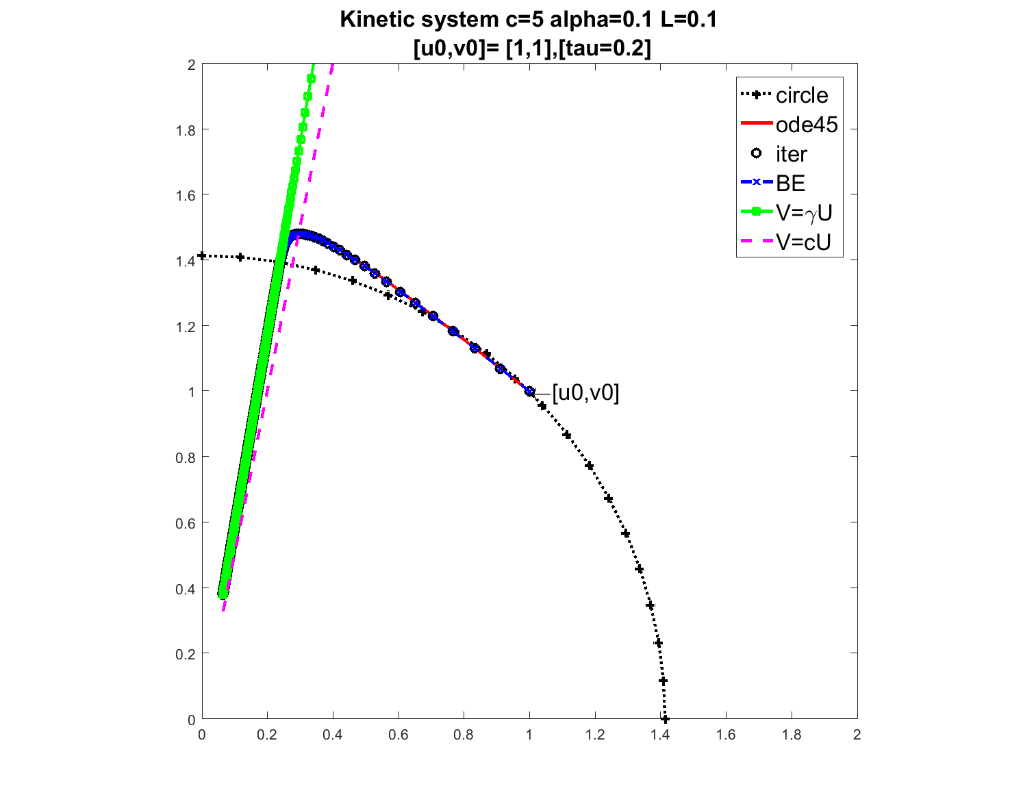
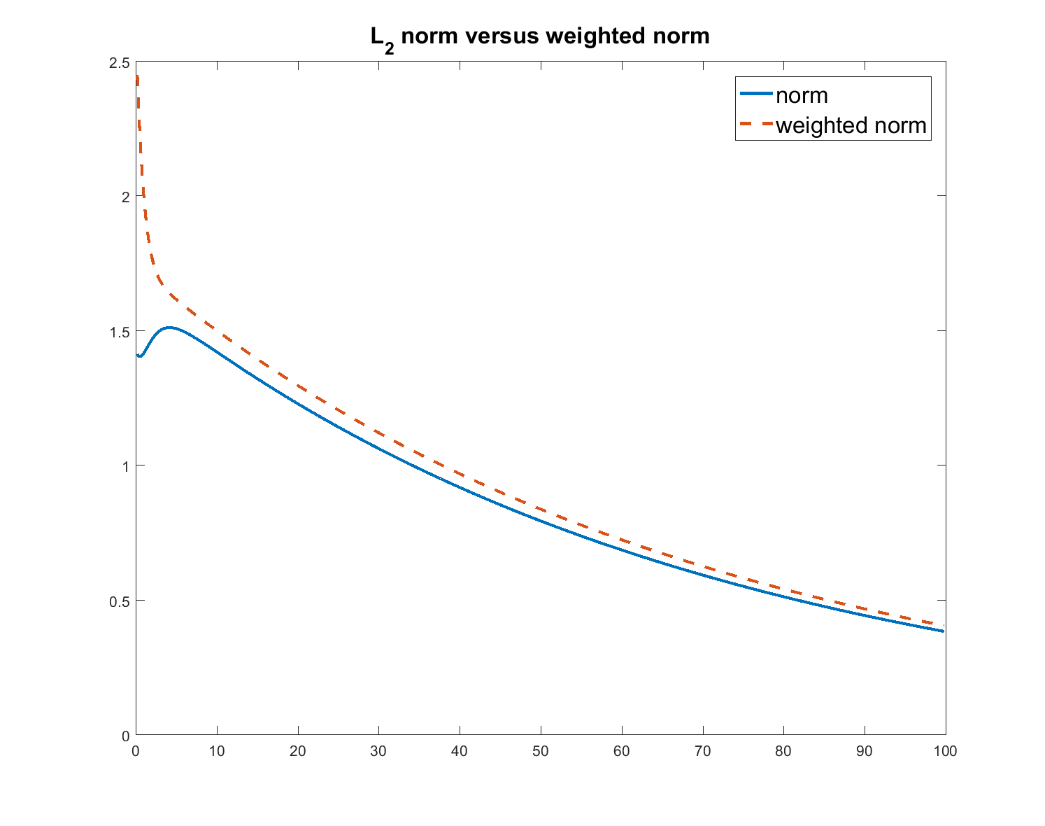
Figure 1: Illustration of the lack of strong stability discussed in Sec. 5.1. Left: the phase plot $(u,v)$ shows that the norm ${\parallel\!w\!\parallel}_{H\times H}$ does not necessarily decrease. Right: the plot of the weighted norm ${\parallel\!w\!\parallel}_{W_{c}}(t)$ decreases while ${\parallel\!w\!\parallel}_{H\times H}(t)$ does not.

5.2 Convergence of the schemes for advection and for diffusion

With the stability results developed above, we expect the error for the case $L=A$ to be of first order, as long as the true solution is smooth enough. While the study of the regularity of the solutions is outside the scope of this paper, we see that the case $L=A$ with Riemann data develops enough smoothness to warrant first order error in all $L_{p}$ spaces $1\leq p<\infty$ and even for $p=\infty$, similarly to what was observed in [5]. In turn, for $L=D$, with optimal smoothness, we expect second order convergence, which is confirmed.

To test convergence, we use fine grid solution $u_{h_{fine}}$ instead of manufacturing solutions which would require nonhomogeneous right-hand side in (7b). To simplify matters, we only report on convergence rate at a fixed stopping time $T$.

We define the error quantities (classical, and new quantity of interest)

$$E_{CQ}=\sqrt{{\|u-u_{h}\|}_{L_{2}}^{2}+{\|v-v_{h}\|}_{L_{2}}^{2}},$$ (57)

$$E_{QoI}=\sqrt{c{\|u-u_{h}\|}_{L_{2}}^{2}+{\|v-v_{h}\|}_{L_{2}}^{2}},$$ (58)

where the $L_{p}$ grid norm for $1\leq p<\infty$ is defined , as usual

$${\|u-u_{h}\|}_{L_{p}}=(\sum_{i}h{|u(x_{i},T)-u_{h}(x_{i},T)|}^{p})^{1/p}.$$ (59)

In tables below, we report on the errors in different quantities of interest $E_{r}$ as well is in different norms ${\parallel\!\cdot\!\parallel}{p}$, and calculate the respestive orders of the error $\alpha_{r}$, $\alpha_{p}$.

5.2.1 Advection case

We consider the problem

$$u_{t}+v_{t}+u_{x} = 0,x\in\mathbf{R}$$

$$v_{t}+\alpha(v-cu) = 0.$$

and its approximation by the upwind scheme (51). To satisfy the CFL condition, we use $\lambda=0.99$, and we vary $\tau$ with $h$ in convergence terst. We choose intial data

$$u(x,o)=\mbox{``box''}(x)=\begin{cases}1&\mbox{ if }x\in[-1,0]\\ 0&\mbox{ otherwise}\end{cases}.$$ (60a)

and $$c=0.1,\,\alpha=2$$. We also set

$$v(x,0)=cu(x,0).$$ (60b)

which coresponds to (6). This helps to relate our convergence rates to those obtained in [5].

Since the true solution is not known, we use $M_{fine}=5050$ and $T=4.8$. In Table 2 we show that the error in every quantity of interest is of first order.

M	${\|u-u_{h}\|}_{L_{2}}$	$\alpha_{L_{2},u}$	${\|v-v_{h}\|}_{L_{2}}$	$\alpha_{L_{2},v}$	${\|u-u_{h}\|}_{L_{1}}$	$\alpha_{L_{1},u}$
20	0.03682	-	0.004641	-	0.06217	-
50	0.01655	0.8728	0.002557	0.6504	0.02607	0.9483
100	0.007575	1.127	0.0009912	1.367	0.01281	1.026
200	0.003687	1.039	0.0004855	1.03	0.006244	1.036
500	0.001329	1.113	0.0001771	1.101	0.002254	1.112

M	${\|u-u_{h}\|}_{\infty}$	$\alpha_{\inf}$	$E_{CQ}$	$\alpha_{CQ}$	$E_{QoI}$	$\alpha_{QoI}$
20	0.03396	-	0.03711	-	0.1221	-
50	0.02598	0.2922	0.01674	0.8685	0.05488	0.8728
100	0.007129	1.866	0.00764	1.132	0.02512	1.127
200	0.003529	1.014	0.003719	1.038	0.01223	1.039
500	0.001331	1.064	0.001341	1.113	0.004409	1.113

Table 2: Errors for advection case, with parameters $c=0.1,\,\alpha=2$, and “box” as the initial condition. Here $M_{fine}=5050$ and $T=4.8$

5.2.2 Convergence for diffusion

We consider the problem

$$u_{t}+v_{t}-u_{xx} = 0,x\in(0,1)$$

$$v_{t}+\alpha(v-cu) = 0.$$

with the homogenous Dirichlet boundary conditions, and initial conditions

$$u(x,0)=\mbox{``bell''}=\exp\left(-{(x-0.5)}^{2}/0.3\right).$$ (62a)

$$v(x,0)=cu(x,0).$$ (62b)

In all experiments for this case we use $d=2$, stopping time $T=3.2$ and $M_{fine}=2000$. We vary $\tau=O(h^{2})$ and expect optimal second order convergence. Indeed, Table 3 shows that error is $O(h^{2})$ in every quantity of interest.

M	${\|u-u_{h}\|}_{L_{2}}$	$\alpha_{L_{2},u}$	${\|v-v_{h}\|}_{L_{2}}$	$\alpha_{L_{2},v}$	${\|u-u_{h}\|}_{L_{1}}$	$\alpha_{L_{1},u}$
20	0.001785	-	0.01447	-	0.002758	-
50	0.000285	2.003	0.002308	2.003	0.0004424	1.997
100	5.002$\cdot 10^{-5}$	2.51	0.0003468	2.734	8.73$\cdot 10^{-5}$	2.341
200	1.253$\cdot 10^{-5}$	1.997	8.657$\cdot 10^{-5}$	2.002	2.195$\cdot 10^{-5}$	1.992

M	${\|u-u_{h}\|}_{\infty}$	$\alpha_{\inf}$	$E_{CQ}$	$\alpha_{CQ}$	$E_{QoI}$	$\alpha_{QoI}$
20.0	0.001849	-	0.01458	-	0.004373	-
50.0	0.0002954	2.002	0.002326	2.003	0.000698	2.003
100.0	4.274$\cdot 10^{-5}$	2.789	0.0003504	2.73	0.0001225	2.51
200.0	1.067$\cdot 10^{-5}$	2.002	8.748$\cdot 10^{-5}$	2.002	3.07$\cdot 10^{-5}$	1.997

Table 3: Errors for diffusion case, with parameters $c=5,\,\alpha=1.2$, and the “bell” as the initial condition. Here $M_{fine}=2000$; $T=3.2$

5.3 Illustration of equilibrium vs non-equilibrium models

Now we are ready to show simulation results which illustrate the kinetic effects in contrast to the equilibrium case. They are most interesting for $L=A$, similar to (51). We use $\Omega=(-1,3)$ and periodic boundary conditions for $u$. We set $\alpha=2$ and $c=0.5$.

Fig. 2 shows the evolution of $[u(x,t),v(x,t)]^{T}$ at three time steps as shown. In addition, we show the evolution of an equilbrium solution in which $\alpha\to\infty$.

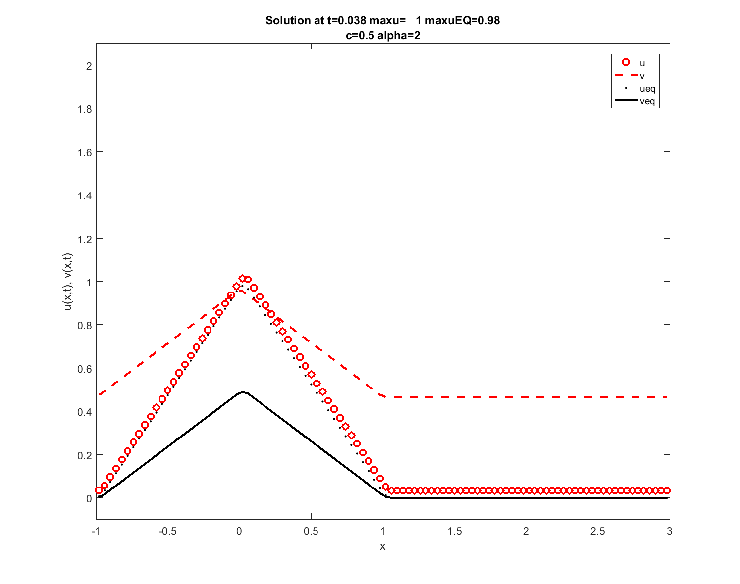
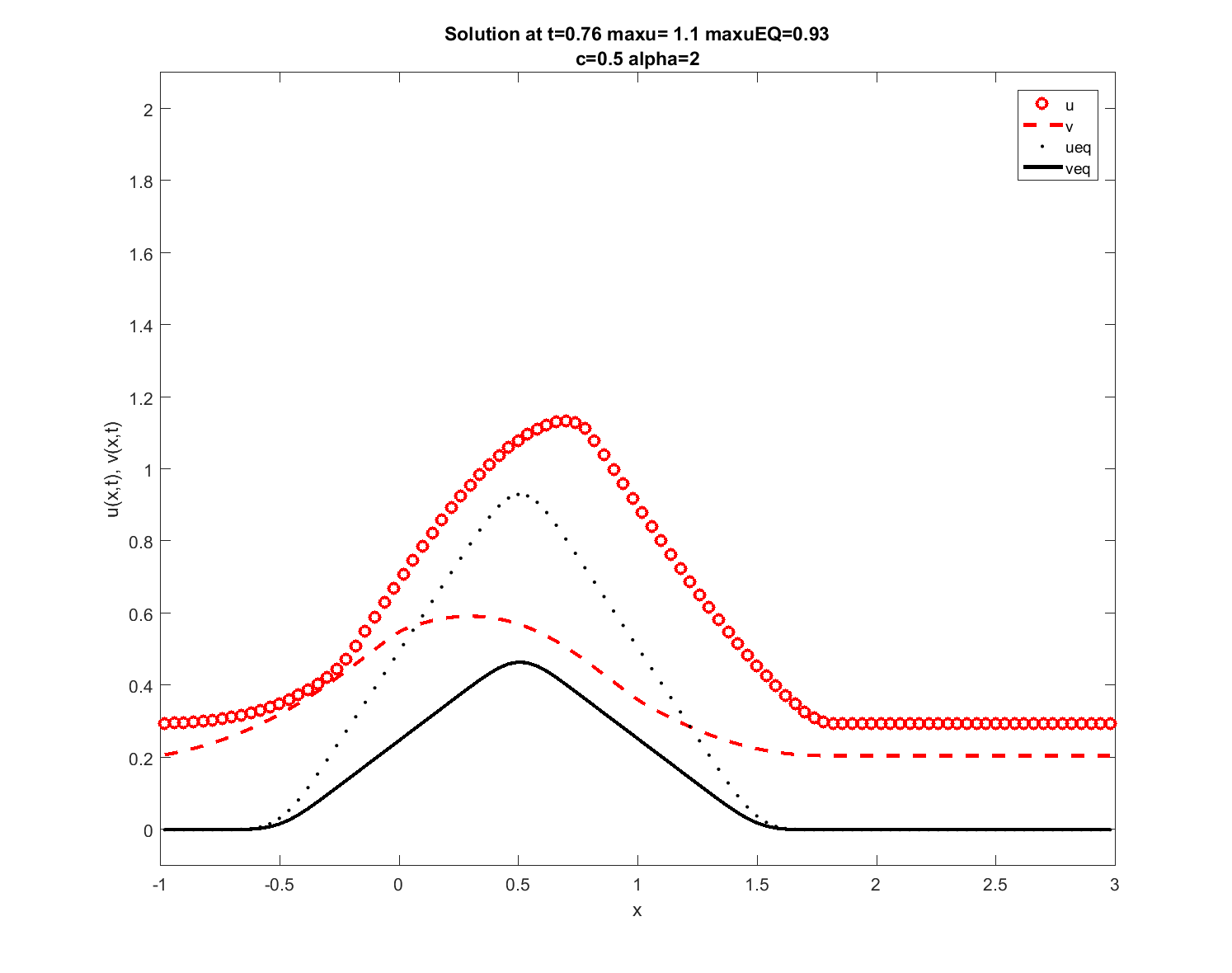
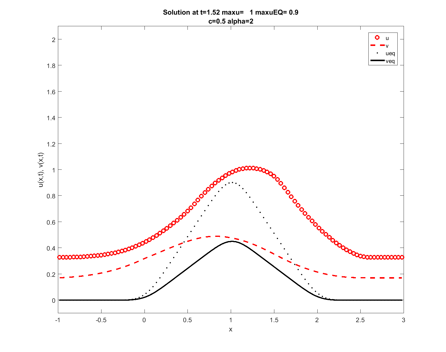
Figure 2: Evolution for $L=A$ described in Sec. 5.3.

6 Extensions

Above we have shown a unified framework for the analysis of explicit-implicit schemes for the kinetic problems with a linear non-equilibrium relationship. Further work is underway to generalize these results, see below for nonlinear systems and systems with multiple immobile sites. Error analysis and stability for time-discrete schemes is underway.

6.1 Nonlinear equilibrium

Here we consider the nonlinear extension of (2) in which $cU$ in (2b) is replaced by $g(u)$, with a monotone increasing function $g:\mathbf{R}\mapsto R$. We only consider a finite dimensional case and $H=\mathbf{R}^{P}$ since the proper setup with nonlinearity in, e.g., $L^{2}(\Omega)$ is extensive and outside the present scope. Here $g(U)=(g(u_{j}))_{j},u\in\mathbf{R}^{P}$ is understood pointwise. The problem is

$$U^{\prime}-\alpha(V-g(U))+LU = 0$$ (63a)

$$V^{\prime}+\alpha(V-g(U)) = 0,$$ (63b)

and we will show stability of a particular new quantity of interest.

Lemma 2

Let $L$ and $g$ satisfy

$$\langle LU,g(U)\rangle\geq 0$$ (64)

Then it holds that

$$\frac{d}{dt}\left[G(U)+\frac{1}{2}{\parallel\!V\!\parallel}^{2}\right]\leq 0.$$ (65)

where $G$ is the primitive of $g(\cdot)$.

Proof: To show the stability, we take the inner product of (63a) with $g(U)$ and of (63b) with $V$

$$\langle U^{\prime},g(U)\rangle-\alpha\langle V,g(U)\rangle+\alpha\langle g(U),g(U)\rangle+\langle AU,g(U)\rangle = 0$$

$$\langle V^{\prime},V\rangle+\alpha\langle V,V\rangle-\alpha\langle g(U),V\rangle = 0.$$

Adding the two equations up we have

$$\langle U^{\prime},g(U)\rangle+\langle V^{\prime},V\rangle+\alpha\langle V,V\rangle-2\alpha\langle V,g(U)\rangle+\alpha\langle g(U),g(U)\rangle+\langle AU,g(U)\rangle=0.$$

Rewriting we obtain

$$\langle U^{\prime},g(U)\rangle+\langle V^{\prime},V\rangle+\alpha\left[\langle V-g(U),V-g(U)\rangle\right]+\langle LU,g(U)\rangle=0.$$

Next step is to define a primitive $G:\mathbf{R}\to R$ of $g(\cdot)$ so that $G^{\prime}(r)=g(r)$ and $\frac{d}{dt}G(U_{j})=g(u_{j})\frac{d}{dt}u_{j}$. We can thus write $\langle U^{\prime},g(U)\rangle=\frac{d}{dt}\sum_{j}G(u_{j})$.

Thus, if (64) holds, we obtain stability since and we have proven Lemma 2.

Next we provide sufficient conditions for (64) to hold. By a difference matrix [31] we mean $D:\mathbf{R}^{N}\mapsto R^{N+1}$ such that $(Du)_{j}=u_{j}-u_{j-1}$ for $j=2,\ldots N-1$, and $(Du)_{1}=u_{1},(Du)_{N+1}=-u_{N}$. $D$ is therefore a discrete analogue of the derivative (gradient). In turn, $D^{T}:\mathbf{R}^{N=1}\mapsto\mathbf{R}^{N}$ which satisfies $(DU,V)_{R^{N+1}}=(U,D^{T}V)_{R^{N}}$, for any $U\in R^{N}$ and $V\in R^{N+1}$, is the discrete analogue of the negative of the divergence, which is dual to the gradient. (The analogues make sense if one also assumes that $u_{0}=0$ and $u_{N+1}=0$, i.e., imposes homogeneous Dirichlet boundary conditions on $U$.)

Proposition 3

Let $L=D^{T}KD$ where $D$ is a difference matrix, and $K$ is a diagonal matrix with positive entries. Then (64) holds.

Proof: It remains to prove that $L=D^{T}KD$ satisfies (64). We consider first the case when $K=I$. The matrix $D^{T}D$ is the well known “discrete Laplacian” $L_{h}$ in Section 4.2 which is symmetric positive definite, and it is easy to see that $(D^{T}Du,u)_{R^{N}}=(Du,Du)_{R^{N+1}}=u_{1}^{2}+\sum_{j=2}^{N}(u_{j}-u_{j-1})^{2}+U_{N}^{2}>0$ unless $U=0$. Similarly we obtain $(D^{T}DU,g(U))_{R^{N}}=(DU,Dg(U))_{R^{N+1}}=u_{1}g(u_{1})+\sum_{j=2}^{N}(u_{j}-u_{j-1})(g(u)-g(u_{j-1})+u_{N}g(u_{N})$ which is nonnegative by virtue of $g(\cdot)$ being a monotone increasing function.

In the more general case when $K\neq I$ we see that the argument above holds for diagonal matrix $K$ with the the entries $k_{1},\ldots k_{N+1}$. Then we obtain $(D^{T}KDu,g(u))_{R^{N}}=k_{1}u_{1}g(u_{1})+\sum_{j=2}^{N}(k_{j})(u_{j}-u_{j-1})(g(u)-g(u_{j-1})+k_{N+1}u_{N}g(u_{N})$. Since each of these entries is nonnegative, we obtain the desired result.

6.2 Stability for a system with two species

Here we consider again the finite dimensional space $H=\mathbf{R}^{n}$ and write

$$U^{\prime}+V_{1}^{\prime}+V_{2}^{\prime}+LU = 0$$ (66)

$$V_{1}^{\prime}+\alpha_{1}(V_{1}-c_{1}U) = 0$$ (67)

$$V_{2}^{\prime}+\alpha_{2}(V_{2}-c_{2}U) = 0$$ (68)

Here we take the inner product of the first equation with $c_{1}c_{2}U$, the second by $c_{2}V_{1}$, the third by $c_{1}V_{2}$, (notice the crossmultiplications) and add up to get

$$c_{2}V_{1}^{T}V_{1}+c_{2}V_{2}^{T}V_{2}+c_{1}c_{2}U^{T}U+c_{1}c_{2}LU^{2}$$

$$+\alpha_{1}c_{2}(V_{1}-c_{1}U)^{2}+\alpha_{2}c_{1}(V_{2}-c_{2}U)^{2}=0$$

from which the stability follows for the following quantity

$$\frac{d}{dt}\left(c_{1}c_{2}{\parallel\!U\!\parallel}^{2}+c_{2}{\parallel\!V_{1}\!\parallel}^{2}+c_{1}{\parallel\!V_{2}\!\parallel}^{2}\right)\leq 0.$$ (69)

Further extensions to $m$ species are possible but will not be discussed.

7 Acknowledgements

The authors would like to thank the anonymous reviewers whose remarks helped to improve the paper.

Research presented in this paper was partially supported by NSF grants DMS-1115827 “Hybrid modeling in porous media”, and DMS-1522734 “Phase transitions in porous media across multiple scales”; second author served as a Principal Investigator on these projects. Majority of research was done when first author F. Patricia Medina was a PhD student and later a faculty at Oregon State University.