The SNPR neighbourhood of tree-child networks

Abstract

Network rearrangement operations like SNPR (SubNet Prune and Regraft), a recent generalisation of rSPR (rooted Subtree Prune and Regraft), induce a metric on phylogenetic networks. To search the space of these networks one important property of these metrics is the sizes of the neighbourhoods, that is, the number of networks reachable by exactly one operation from a given network. In this paper, we present exact expressions for the SNPR neighbourhood of tree-child networks, which depend on both the size and the topology of a network. We furthermore give upper and lower bounds for the minimum and maximum size of such a neighbourhood.

1 Introduction

Phylogenetic trees and networks are used to represent and study the evolutionary relationships of species and languages. The set of all hypothesised networks to model the relationships for a set of data is referred to as a space of phylogenetic networks. To navigate and work with such a space one common tool is using rearrangement operations that transform one network into another one and thereby induce a metric on the space. For phylogenetic trees three well known such operations are the Nearest Neighbour Interchange (NNI) [20], the Subtree Prune and Regraft (SPR) and Tree Bisection and Reconnection (TBR) [1] operations. In recent years, the study of rearrangement operations has moved from the tree space to the network space. For example, the NNI operation has been generalised from trees to networks by Huber et al. [13], and further considered in its unrooted variant [14, 9] and its rooted variant [12, 17]. Francis et al. [9] also introduced SPR and TBR on unrooted phylogenetic networks. Furthermore and as with this paper, the generalisation of rSPR (rooted SPR) operation for rooted phylogenetic networks has been studied. Bordewich et al. [3] introduced the SubNet Prune and Regraft (SNPR) operation, which allows to navigate between phylogenetic networks with both the same and with different number of reticulations. Gambette et al. [12] and Janssen et al. [17] studied a slightly more powerful rSPR operation (reusing the original name) for phylogenetic networks with the same number of reticulations.

An interesting property of these operations and spaces is the sizes of a neighbourhood of a network. The neighbourhood problem with respect to a type of operation asks how many networks in the space are exactly one such operation apart from a given network. Robinson [20] already considered this question when he laid the foundation for the studies of rearrangement operations with the introduction of NNI on unrooted phylogenetic trees. Allen and Steel [1] solved the problem for SPR on unrooted phylogenetic trees. The size of the neighbourhood of an unrooted phylogenetic tree, for both NNI and SPR, only depends on the number of leaves of the tree. However, Allen and Steel [1] further showed that for unrooted trees and TBR, the size of the neighbourhood depends not only on the number of leaves but also on the topology of the tree. Humphries and Wu [15] later gave a closed formula for the neighbourhood under TBR using the non-trivial splits of a tree to represent the topology. Beyond that, Baskowski et al. [2] considered the problem for SPR and TBR on unrooted phylogenetic trees that are restricted to a circular ordering of its leaves, and de Jong et al. [8] considered the problem of finding neighbours that are two or more operations away for an unrooted phylogenetic tree. For rooted phylogenetic trees and rSPR the size of the neighbourhood depends again on the number of leaves, but also on the topology of the tree. Song [21] gave a formula for this problem where he characterises the size by the number of ancestors of each vertex in a tree. He used a recursive approach to count neighbours, which he then transformed into a closed formula. Furthermore, Song [22] did the same for totally ordered phylogenetic trees.

The problem of determining the neighbourhood size gets harder for phylogenetic networks. Huber et al. [13] solved the problem for NNI operations on unrooted level-1 networks. They showed that the size depends on structures of the network like the number of cycles of size three and four. Gambette et al. [12] extended this with an upper bound for the neighbourhood size of an unrooted phylogenetic network and NNI, but restricted to networks with a fixed number of reticulations. Similarly, Francis et al. [9] gave an upper bound for the same networks but for SPR instead of for NNI. In this paper, we will show that for rooted phylogenetic networks and SNPR the neighbourhood size depends on the number of leaves, the topology of the network in terms of descendants and occurrences of certain structures. We will outline why identifying these structures is difficult for rooted phylogenetic networks in general and for the classes of tree-based [10] and reticulation-visible [16] networks. However, for classes like tree-child [24], normal [25] and level-1 [11] networks, the dependencies of the neighbourhood size on the topology are comprehensible. We will focus on the class of tree-child networks, a class for which several problems that are difficult in general can be solved efficiently [23, 7, 4, 5]. The class of tree-child networks is also not as restricted as normal and level-1 networks, which are in fact subclasses of it. The main result of this paper is a formula for the neighbourhood size of a tree-child network under SNPR. As byproduct we reprove the formula for rooted phylogenetic trees by Song. We also give bounds on the neighbourhood size that only depend on the number of leaves (Section 4). First, however, we introduce the notation and terminology used throughout this paper.

2 Preliminaries

We now recall the definitions of rooted phylogenetic networks, the class of tree-child networks, and the SNPR and NNI operations. We also formally define the unit neighbourhood problem and structures of a phylogenetic network like triangles, diamonds and trapezoids.

Phylogenetic networks.

A rooted binary phylogenetic network $N=(V,E)$ is a directed acyclic graph with edges $E$ and the following vertices $V$:

• the root $\rho$ with in-degree zero and out-degree one,

• $n$ leaves with in-degree one and out-degree zero bijectively labelled with a set of taxa,

• inner tree vertices with in-degree one and out-degree two, and

• reticulations with in-degree two and out-degree one.

The tree vertices of $N$ are the union of the inner tree vertices, the leaves and the root. The unique edge incident to the root is called the root edge $e_{\rho}$. An edge $e=(u,v)$ is called a reticulation edge, if $v$ is a reticulation, and a tree edge, if $v$ is a tree vertex. An edge not incident to the root or a leaf is an inner edge. Furthermore, we call $e=(u,v)$ pure, if $u$ and $v$ are both either tree vertices or reticulations, and impure otherwise. Throughout this paper we assume that $n\geq 2$ and let $r$ denote the number of reticulations. There are thus $m=2n+3r-1$ edges in $N$ [19, Lemma 2.1].

Our definition of a rooted binary phylogenetic network allows the existence of parallel edges. Furthermore, we note that our definition of the root is known as pendant root [3] and that it differs from another common definition where the root has out-degree two. Our variation serves both elegance and technical reasons. Since we only consider a fixed set of taxa, we omit its notation. Moreover, throughout this paper we only consider phylogenetic networks that are both rooted and binary and therefore refer to them simply as phylogenetic networks.

Let $N$ be a phylogenetic network. For two vertices $u$ and $v$ in $N$, we say that $u$ is a parent of $v$ and $v$ is a child of $u$, if there is an edge $(u,v)$ in $N$. We say $u$ is ancestor of $v$ and $v$ is descendant of $u$ if there is a directed path from $u$ to $v$ in $N$. We say $u$ and $v$ are siblings if they have a common parent. For ease of use, we also say that $u$ is an uncle of $v$, if $u$ is sibling of a parent of $v$. In reverse, $v$ is then the nephew of $u$.

Let $(u,v),(x,y)$ be edges of $N$. We say $(x,y)$ is a parent edge of $(u,v)$ if $y=u$. Consequently, $(u,v)$ is then a child edge of $(x,y)$. The two edges are considered siblings if $u=x$. We say $(u,v)$ is a descendant of $(x,y)$ if either $y=u$ or if $u$ is a descendant of $y$. In return, $(x,y)$ is then an ancestor of $(u,v)$. For an edge $e$ of $N=(V,E)$ we use the function $\delta\colon E\to\mathbb{N}$ to count the number of descendant edges of $e$, i.e. $\delta(e):=\lvert\{f\in E\mid f\text{ is descendant of }e\}\rvert$. For example, in the phylogenetic network $N_{2}$ in Figure 1 the edge $g$ has $\delta(g)=5$ descendants and the root edge $e_{\rho}$ has $\delta(e_{\rho})=2n+3r-2=17$ descendants. We note that we do not consider a vertex or an edge to be its own ancestor or descendant.

Network classes.

A phylogenetic network that has no reticulations is called a rooted binary phylogenetic tree, or in this paper simply a phylogenetic tree. A phylogenetic network in which every non-leaf vertex has a tree vertex as child is a tree-child network. We denote by $\mathcal{N}_{n}$ all phylogenetic networks with $n$ leaves, and with $\mathcal{T}_{n}$ and $\mathcal{TC}_{n}$ the subsets of $\mathcal{N}_{n}$ consisting of all phylogenetic trees and tree-child networks, respectively.

One important well known property of tree-child networks is that each vertex $v$ contains a path to a leaf consisting only of tree edges. Such a path is called a tree path of $v$. Another property is that a tree-child network has at most $n-1$ reticulations [6, Proposition 1].

A symmetry of a phylogenetic network $N$ can be interpreted as an automorphism on $N$, distinct from the identity function, that fixes the leaf set of $N$. The next proposition shows that tree-child networks have no such symmetries. It is a reformulation of a result by McDiarmid et al. [19, Lemma 5.1]. This implies that every vertex and every edge of a tree-child network is uniquely identifiable, for example recursively by its set of descendant edges.

Proposition 1

Let $N\in\mathcal{TC}$.

Then $N$ has exactly one automorphism that fixes its leaf set.

Note that it can also be shown that so-called normal networks, tree-sibling networks and level-1 networks without parallel edges have no such symmetries [18]. We will see why this is favourable for counting neighbours in the next section, and discuss at the end, in Section 5, why the problem gets harder for more complex networks, which can have such symmetries.

Suboperations.

To define SNPR operations we first have to define several suboperations. Let $G$ be a directed acyclic graph. A degree-two vertex $v$ of $G$ with parent $u$ and child $w$ gets suppressed by deleting $v$ and the edges $(u,v)$ and $(v,w)$ and adding the edge $(u,w)$. An edge $(u,w)$ of $G$ gets subdivided by adding a new vertex $v$, deleting the edge $(u,w)$ and adding the edges $(u,v)$ and $(v,w)$. Hence, a subdivision is the reverse of a suppression.

Let $N$ be a phylogenetic network. We say that an edge $e=(u,v)$ of $N$ with $u$ not a reticulation gets pruned by transforming it into the half edge $(.,v)$ and suppressing $u$. In reverse, we say a half edge $(.,v)$ gets regrafted to an edge $(u,w)$ by becoming the edge $(u^{\prime},v)$ where $u^{\prime}$ is a new vertex subdividing $(u,w)$.

SNPR.

Let $N\in\mathcal{N}_{n}$. Let $e=(u,v)$ with $u$ not a reticulation and $f=(x,y)$ an edge that is not a descendant edge of $e$. Then, like Bordewich et al. [3], we define the SubNet Prune and Regraft (SNPR) operation that transforms $N$ into a phylogenetic network $N^{\prime}\in\mathcal{N}_{n}$ by applying exactly one of the following three operations:

1. If $f\neq e$, an SNPR operation $(e,f)$ prunes $e$ and regrafts it to $f$.

2. If $f\neq e$, an SNPR$+$ operation $(e,f)$ subdivides $f$ and $e$ with new vertices $u^{\prime}$ and $v^{\prime}$, respectively, and adds the edge $(u^{\prime},v^{\prime})$. If $e=f$, an SNPR$+$ operation $(e,f)$ subdivides $e$ twice with $u^{\prime}$ and $v^{\prime}$ such that $u^{\prime}$ is parent of $v^{\prime}$, and adds the edge $(u^{\prime},v^{\prime})$.

3. If $e$ is a reticulation edge, an SNPR$-$ operation $(e)$ deletes $e$ and suppresses $u$ and $v$.

For an SNPR operation $(e,f)$ (or equivalently for other types of operations), we write $(e,f)(N)$ to denote the phylogenetic network $N^{\prime}$ that results from applying $(e,f)$ to $N$. We note that SNPR is for rooted phylogenetic trees indeed a generalisation of rSPR. Bordewich et al. [3] have shown that the three types of SNPR operations are reversible. This means that for every SNPR operation that transforms $N$ into $N^{\prime}$, there exists an SNPR operation that transforms $N^{\prime}$ into $N$, and that for every SNPR$+$ operation, there exists an inverse SNPR$-$ operation, and vice versa. The SNPR operation induces thus a distance function and a metric on $\mathcal{N}_{n}$. Bordewich et al. [3] also showed that $\mathcal{N}_{n},\mathcal{T}_{n}$ and $\mathcal{TC}_{n}$ and other classes are connected under SNPR. Moreover, they showed that the corresponding diameter of $\mathcal{TC}_{n}$ is linear in $n$.

Figure 1: The phylogenetic network $N_{2}$ can be obtained from $N_{1}$ by the SNPR operation $(e,f)$. The phylogenetic network $N_{3}$ can be obtained from $N_{2}$ with the SNPR$-$ operation $(g)$. Both operations have a corresponding SNPR and SNPR$+$ operation, respectively, that reverses the transformation.

NNI.

The Nearest Neighbour Interchange (NNI) operation was defined on (unrooted) phylogenetic trees [20], but has recently been generalised to unrooted and rooted phylogenetic networks by Huber et al. [13, 14]. We define the NNI operation here only for tree-child networks, because we will only use it as a tool to count special sets of SNPR operations. Furthermore, our notation and explanation below differ from the one of Huber et al. [13, 14] for technical reasons and since we consider rooted phylogenetic networks.

Let $N\in\mathcal{TC}_{n}$ and $e=(u,v)$ be an edge of $N$. Note that $e$ can not be a pure reticulation edge, since $N$ is tree child. If $e$ is an inner edge, let $g\neq e$ be an edge incident to $v$. If $u$ is a tree vertex, let $f$ be the sibling edge of $e$ and otherwise a parent edge of $e$. Then we define the Nearest Neighbour Interchange (NNI) operation that transforms $N$ into $N^{\prime}\in\mathcal{TC}_{n}$ by applying exactly one of the following three operations:

1. If $e$ is an inner tree edge, an NNI operation $(f,e,g)$ prunes $g$ and regrafts it to $f$, and, if $e$ is a reticulation edge, prunes $f$ and regrafts it to $g$.

2. An NNI$+$ operation $(e,f)$ subdivides $f$ with vertex $u^{\prime}$ and $e$ with vertex $v^{\prime}$, and adds the edge $(u^{\prime},v^{\prime})$.

3. If $e$ is the long side of a triangle (defined later), an NNI$-$ operation $(e)$ deletes $e$ and suppresses $u$ and $v$.

The edge $e$ is called the axis of the NNI operation $(f,e,g)$. Note that our definitions allow that $N^{\prime}=N$. Figure 2 illustrates the three types of NNI operations. We note that all three types of NNI operations are special cases of SNPR operations. Furthermore, like for SNPR, we observe that NNI operations are reversible and that NNI$+$ and NNI$-$ operations are mutually inverse.

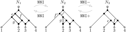
Figure 2: The phylogenetic network $N_{2}$ can be obtained from $N_{1}$ by the NNI operation $(f,e,g)$. $N_{3}$ can be obtained from $N_{2}$ with the NNI$-$ operation $(g)$. Both operations have a corresponding NNI operation $(f^{\prime},e^{\prime},g)$ and NNI$+$ operation $(e,f)$, respectively, that reverses the transformation.

Neighbourhood.

Two phylogenetic networks that are one SNPR operation apart are called SNPR neighbours. The unit SNPR neighbourhood $U_{\textup{SNPR}}(N)$ of $N$ is the set of all SNPR neighbours of $N$. When we consider a tree-child network $N$, we are only interested in neighbours that are also tree child. We call this neighbourhood the unit SNPR tree-child neighbourhood and denote it by $U_{\textup{SNPR}}^{\mathcal{TC}}(N)$. Figure 3 gives an example of a tree-child network and its unit tree-child SNPR neighbourhood.

For $N\in\mathcal{N}_{n}$, we denote by $\Theta_{\textup{SNPR}}(N)$ the set of all SNPR operations on $N$. (This can, in fact, be a multi-set, since $(e,f)$ can denote an SNPR or an SNPR$+$ operation.) An operation on a tree-child network that yields again a tree-child network is called tree-child respecting. If $N\in\mathcal{TC}_{n}$, we write $\Theta_{\textup{SNPR}}^{\mathcal{TC}}(N)$ to denote the set of tree-child-respecting SNPR operations on $N$. The definitions for $\mathcal{T}_{n}$ and SNPR, SNPR$+$, and SNPR$-$ are analogous.

An operation $\theta\in\Theta_{\textup{SNPR}}(N)$ is called trivial, if $\theta(N)=N$. Furthermore, we call two distinct operations on $N$ redundant, if they yield the same phylogenetic network $N^{\prime}$. A set of pairwise redundant operations is called a redundancy set. Note that $\lvert\Theta_{\textup{SNPR}}(N)\rvert\geq\lvert U_{\textup{SNPR}}(N)\rvert$, since there can be trivial operations and redundancy sets.

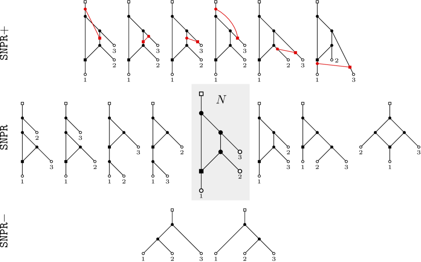
Figure 3: A tree-child network $N$ in the middle, with its SNPR tree-child neighbourhood around it. The top row consists of the SNPR$+$ neighbours, the middle row of the SNPR neighbours, and the bottom row of the SNPR$-$ neighbours.

Structures.

Let $N\in\mathcal{TC}_{n}$. In the following we define certain subgraphs of $N$, which we call structures, that are the determining factor of whether operations on $N$ are tree-child respecting, trivial and redundant. Figure 4 accompanies our description of these structures.

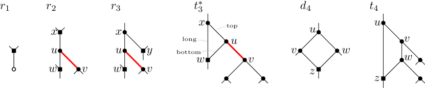
Figure 4: An $r_{1}$, $r_{2}$, and $r_{3}$ structure, a tree-branching triangle $t_{3}^{*}$, a diamond $d_{4}$, a trapezoid with outgoing tree edges $t_{4}$. The critical edges (bold red) and the paths between the reticulations of the $r_{2}$ and $r_{3}$ structure are highlighted.

An $r_{2}$ structure of $N$ is a path of length two from a reticulation $x$ via a vertex $u$ to a reticulation $w$. An $r_{3}$ structure consists of four vertices $x,y,u,w$ with edges $(x,y)$, $(x,u)$ and $(u,w)$ where $y$ and $w$ are reticulations. We refer to the undirected path $w,u,x,y$ as the underlying path of the structure. Note that in both an $r_{2}$ and an $r_{3}$ structure, since $N$ is tree child, both $u$ and its second child $v$ are tree vertices. We abuse the notation to denote by $r_{2}$ and $r_{3}$ also the number of these structures in $N$. We define $r_{1}$ as the number of reticulations in $N$ whose child is a leaf.

Note that an $r_{3}$ structure with $y=w$ is a triangle. Formally, a triangle of $N$ consist of three vertices $x,u,w$ with the edges $(x,u)$, $(x,w)$ and $(u,w)$. We call the edge $(x,u)$ the top side, $(x,w)$ the long side, and $(u,w)$ the bottom side of the triangle. We denote the number of triangles in $N$ by $t_{3}$. Furthermore, let $v\neq w$ be the second child of $u$. We note that since $N\in\mathcal{TC}_{n}$, we know that $u$ is a tree vertex. Then if $v$ is incident to three pure tree edges, we call the triangle a tree-branching triangle. We denote the number of those by $t_{3}^{*}$. We want to point out that every tree-branching triangle of $N$ is counted as an $r_{3}$ structure, as a triangle and as a tree-branching triangle.

For an $r_{2}$, $r_{3}$ structure, or a triangle, with the notation from above, we call the tree edge $(u,v)$ the critical edge of this structure. See again Figure 4, where the critical edges are highlighted, and note how pruning them yields a vertex without a tree child. This will be important in the next section when we consider tree-child respecting SNPR operations.

A diamond of $N$ is an undirected four-cycle consisting of edges $(u,v)$, $(u,w)$, $(v,z)$ and $(w,z)$. A trapezoid is an undirected four-cycle consisting of edges $(u,v)$, $(v,w)$, $(w,z)$ and $(u,z)$. We note that in both cases $z$ is a reticulation. Important for us are trapezoids with the outgoing edges of the four-cycle at $v$ and $w$ being pure tree edges. We denote by $d_{4}$ the number of diamonds and with $t_{4}$ the number of trapezoids with two outgoing pure tree edges.

3 SNPR neighbourhood of a tree-child network

Throughout this section let $N\in\mathcal{TC}_{n}$. To count tree-child neighbours of $N$, it is necessary to understand whether an SNPR operation on $N$ results again in a tree-child network, and which operations on $N$ are redundant or trivial. In the following we show that this only depends on different substructures of $N$. We consider SNPR operations first, showing which respect the tree-child property, which are trivial and which are redundant. This then allows us to count the number of neighbours. After that, we include SNPR$+$ and SNPR$-$ operations to consider the SNPR neighbourhood.

Tree-child respecting SNPR operations.

Let $\theta=(e,f)\in\Theta_{\textup{{SNPR}}}^{\mathcal{TC}}(N)$ and $e=(u,v)$. For $\theta$ to respect the tree-child property, neither pruning $(u,v)$ nor then regrafting $(.,v)$ to $f$ can yield a non-leaf vertex without a tree child. Roughly speaking and as we show in the following lemma, this implies that if $e$ is a critical edge, then there are only limited options for $f$, and also that not both $e$ and $f$ can be reticulation edges. Figure 5 illustrates the cases where $e$ is a critical edge.

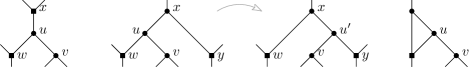
Figure 5: Illustration of the cases $r_{2}$, $r_{3}$, and triangle, where there are only trivial SNPR operations that prune $(u,v)$ or in the case of $r_{3}$ exactly one non-trivial one as shown. This is formalised in Lemma 3.1

Lemma 3.1.

Let $N\in\mathcal{TC}_{n}$ and $(e,f)\in\Theta_{\textup{{SNPR}}}(N)$, $e=(u,v)$, $f=(x,y)$ not a descendant of $e$.

Then $N^{\prime}=(e,f)(N)$ is a tree-child network if and only if one of the following cases holds:

1. $e$ is a reticulation edge and $f$ is not a reticulation edge;

2. $e$ is a pure tree edge that is not critical.

3. $e$ is a critical edge and $f$ is incident to $u$;

4. $e$ is a critical edge of an $r_{3}$ structure with underlying path $w,u,x,y$ such that $u$ and $y$ are the children of $x$ and $f=(x,y)$;

5. $e$ is a critical edge of a triangle and $f$ is the long side of the triangle.

Proof 3.2.

We prove this by considering the different types of $e=(u,v)$. By definition of an SNPR operation, $u$ can not be a reticulation. Thus, $e$ can not be a pure reticulation edge or an impure tree edge. Let $e$ be an impure reticulation edge, i.e. let $v$ be a reticulation. Then, since $N\in\mathcal{TC}_{n}$, the sibling $w$ of $v$ with shared parent $u$ is a tree vertex. Thus after pruning $e$ and suppressing $u$, the parent of $u$ has in $N^{\prime}$ the vertex $w$ as tree child. Hence, a reticulation edge can always be pruned. Now, if $f=(x,y)$ is a reticulation edge, then the new vertex $u^{\prime}$ in $N^{\prime}$, resulting from the subdivision of $f$, has the two children $v$ and $y$, which are both reticulations. Thus, if $e$ is a reticulation edge, $f$ can not be a reticulation edge. If $f$ is not a reticulation edge (Case (i)), then, in $N^{\prime}$, the new vertex $u^{\prime}$ has the tree child $y$, the vertex $x$ has the tree child $u^{\prime}$ and and all other vertices stay unaffected.

Next, let $e$ be a tree edge. Clearly, $e$ is pure. If $e$ is not critical (Case (ii)), then either the sibling of $v$ or the sibling of $u$ is a tree vertex. Without loss of generality let $w$, the sibling of $v$, be a tree vertex. Then, after pruning $e$ and suppressing $u$, the parent $x$ of $u$ has $w$ as a tree child in $N^{\prime}$. Since $v$ is a tree vertex, regrafting $(,v)$ to any edge $f$ does not create a non-leaf vertex without tree child. Hence, $N^{\prime}$ is tree child.

If $e$ is critical and $f$ incident to $e$ (Case (iii)), as $f$ is not a descendant edge of $e$, then $N^{\prime}=N$ and $N^{\prime}$ is thus tree child. If $e$ is the critical edge of an $r_{2}$ structure, then clearly $f$ being incident to $e$ is the only option for $N^{\prime}$ to be tree child. If $e$ is the critical edge of an $r_{3}$ structure, then after pruning $e$ and suppressing $u$, the parent $x^{\prime}$ of $u$ has the two reticulations $y^{\prime}$ and $w$ as children if and only if $e$ is not regrafted to an incident edge and if $f\neq(x^{\prime},y^{\prime})$ (Case (iv)). In the case that the $r_{3}$ structure is a triangle, this yields that $f$ is the long side of the triangle (Case (v)). Since we covered all types of $e$, the described choices of $e$ and $f$ cover all tree-child-respecting SNPR operations.

We now know when exactly an SNPR operation respects the tree-child property. We can thus continue with counting them. Let $E_{R}$ denote all reticulation edges, let $E_{T^{*}}$ denote all pure non-critical tree edges and let $\delta_{T}$ be the restriction of the $\delta$ function that only counts descendant edges that are tree edges.

Lemma 3.3.

Let $N\in\mathcal{TC}_{n}$.

Then the number of tree-child-respecting SNPR operations on $N$ is

$$\begin{split}\lvert\Theta_{\textup{{SNPR}}}^{\mathcal{TC}}(N)\rvert&=4n^{2}+10nr-2n(r_{2}+r_{3})-6n+2r^{2}-3r(r_{2}+r_{3})-5r\\ &\,+4r_{2}+5r_{3}+2-\sum\limits_{e\in E_{T^{*}}}\delta(e)-\sum\limits_{e\in E_{R}}\delta_{T}(e)\text{.}\end{split}$$

Proof 3.4.

Following Lemma 3.1, we prove this by distinguishing different types of the pruned edge $e$. We use the fact that $N$ has $m=2n+3r-1$ edges. First, any reticulation edge $e=(u,v)$ can be regrafted to any non-reticulation edge that is not descendant of $e$. Hence, there are the following many such operations:

$$2r(m-2r)-\sum_{e\in E_{R}}\delta_{T}(e)=4nr+2r^{2}-2r-\sum_{e\in E_{R}}\delta_{T}(e)$$ (1)

Equation 1 uses $\delta_{T}(e)$ instead of $\delta(e)$, since we would otherwise double count the forbidden operations of regrafting to an edge that is reticulation edge and descendant of the pruned edge.

If $e\in E_{T^{*}}$, i.e. a pure non-critical tree edge, then $e$ can be pruned and regrafted to every edge not $e$ itself or a descendant of $e$. Hence, there are the following many such operations:

$$(m-3r-r_{2}-r_{3})(m-1)-\sum_{e\in E_{T^{*}}}\delta(e)\\ =4n^{2}+6nr-2n(r_{2}+r_{3})-6n-3r(r_{2}+r_{3}+1)+2r_{2}+2r_{3}+2-\sum_{e\in E_{T^{*}}}\delta(e)$$ (2)

If $e$ is the critical edge of an $r_{2}$ or $r_{3}$ structure (including triangles), then there are only $2$ or $3$ operations, respectively. Hence, there are the following many such operations:

$$2r_{2}+3r_{3}$$ (3)

Adding Equations 1, 2 and 3 together, the lemma follows.

Trivial SNPR operations.

Pruning an edge and regrafting it at the same edge is a trivial SNPR operation. Another trivial SNPR operation $(e,f)$ arises for every triangle where $e$ is its critical edge and $f$ is its long side. Furthermore, the reticulation edges of a triangle induce a trivial operation each, as the proof of the following lemma shows.

Lemma 3.5.

Let $N\in\mathcal{TC}_{n}$.

Then there are $4n+4r+3t_{3}-4$ trivial operations in $\Theta_{\textup{{SNPR}}}^{\mathcal{TC}}(N)$.

Proof 3.6.

Let $(e,f)\in\Theta_{\textup{{SNPR}}}^{\mathcal{TC}}(N)$ with $e=(u,v)$ and $f=(x,y)$. An operation $(e,f)$ can be trivial in three ways. First, $f$ is incident to $e$ at $u$. The root edge and edges $(u,v)$ with a reticulation $u$ are not prunable. Therefore, there are $m-r-1$ prunable edges and $2(m-r-1)$ trivial tree-child-respecting SNPR operations.

Second, $f$ is isomorphic to the edge $g$ created by pruning $e$ and suppressing $u$. However, this can only happen if $f$ and $g$ are parallel edges, since by Proposition 1 there are no pairs of isomorphic edges in a tree-child network. This means that the critical edge of a triangle gets pruned. Thus, there are $t_{3}$ many trivial SNPR operations of that type.

Third, let $f$ be neither of the above. Let the edges of $N$ be labelled and then in $N^{\prime}=(e,f)(N)$ let all labels be as in $N$ except those affected $(e,f)$. Let the regrafted edge have the label $e$. Then, since $N^{\prime}=N$, there has to be an edge $e^{\prime}=(u^{\prime},v^{\prime})$ in $N^{\prime}$ that is, without label, the same edge as $e$ in $N$. By the choice of $f$, this can not be $e$. The edges $e$ and $e^{\prime}$ got, so to say, swapped. Then, since by Proposition 1 every vertex is unique, $v=v^{\prime}$ follows. The edges $e$ and $e^{\prime}$ are thus reticulation edges. For $N^{\prime}=N$, clearly, $e$ and $e^{\prime}$ have to be the reticulation edges of a triangle: If we prune the long side of a triangle and regraft it to the critical edge of the triangle, it results again in $N$. An equivalent operation exists for the bottom edge of the triangle. Hence, there are $2t_{3}$ such trivial SNPR operations.

Furthermore, these three cases do not overlap and we thus counted all trivial SNPR operations on $N$. Since $2(m-r-1)+3t_{3}=4n+4r+3t_{3}-4$, the lemma follows.

Redundant SNPR operations.

We now consider when and how non-trivial SNPR operation on tree-child networks can be redundant. Humphries and Wu [15] used NNI operations to count redundancies of SPR and TBR operations on unrooted trees. The following lemma states how SNPR and NNI correspond to each other with regards to redundancy on rooted trees.

Lemma 3.7.

Let $T\in\mathcal{T}_{n}$, and let $\theta,\theta^{\prime}\in\Theta_{\textup{{SNPR}}}^{\mathcal{T}}(T)$, $\theta\neq\theta^{\prime}$ be redundant with $\theta(T)=\theta^{\prime}(T)=T^{\prime}\neq T$.

Then there exists an NNI operation $\sigma\in\Theta_{\textup{{NNI}}}^{\mathcal{T}}(T)$ such that $\sigma(T)=T^{\prime}$. Furthermore, every redundancy set of $\Theta_{\textup{{SNPR}}}^{\mathcal{T}}(T)$ has size three.

We prove Lemma 3.7, after we generalise observations on how an SNPR redundancy can occur. Figure 6 illustrates how, in the lemma, three SNPR operations correlate to an NNI operation. There, in the subgraph of $T$, the axis $(x,u)$ of the NNI operation is a pure inner tree edge. We observe that, therefore, such an NNI operation can also induce a redundancy in a phylogenetic network. The edge $(x,u)$ further has the siblings $v$ and $w$ as children of $u$ and their uncle $y$ as child of $x$. Now, the three redundant SNPR operations could be described as follows. First, $((u,v),(x,y))$ prunes $v$ and regrafts it as sibling of $y$. Second, $((x,y),(u,v))$ prunes $y$ and regrafts it as sibling of $v$. Third, $((u,w),(p,x))$ prunes $w$ and regrafts it above $x$, thus makes $v$ and $y$ siblings. In general, to find redundancies of SNPR operations, we can fix two vertices that stand in a certain relation in $N^{\prime}$, but not yet in $N$. Then, to create this relation, say making $v$ and $y$ siblings, we can either regraft one as sibling of the other or alter the path between them. We formalise this with the following lemma, after we precisely describe the initial situation.

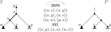
Figure 6: Correlation of an NNI operation with a pure inner tree edge as axis and three SNPR operation, all being pairwise redundant.

Let $N,N^{\prime}\in\mathcal{TC}_{n}$ be neighbours with $N^{\prime}=\theta(N),\theta\in\Theta_{\textup{{SNPR}}}^{\mathcal{TC}}(N)$. Let the vertices in both $N$ and $N^{\prime}$ be labelled and let $\theta$ preserve these labels, except, of course for removed or new vertices. Let now $v$ and $y$ be distinct vertices with the same labels, and such that neither is ancestor of the other in both $N$ and $N^{\prime}$. We now say that $v$ and $y$ are in a desired relation if one of the following holds:

• The vertex $v$ is a sibling, an uncle or a nephew of $y$ in $N^{\prime}$ via a path $P^{\prime}$, but $v$ is in a different relation to $y$ in $N$.

• The vertex $v$ is an uncle or a nephew of $y$ in $N^{\prime}$ via a path $P^{\prime}$ and in $N$ via a path $P\neq P^{\prime}$.

In the second condition, $P\neq P^{\prime}$ means that the labels of the vertices on $P$ differ for a least one vertex from the labels of the vertices on $P^{\prime}$.

Lemma 3.8.

Let $N,N^{\prime}\in\mathcal{TC}_{n}$ and $\theta\in\Theta_{\textup{SNPR}}^{\mathcal{TC}}(N)$ with $\theta(N)=N^{\prime}\neq N$. Let $v$ and $y$ be in a desired relation via the path $P^{\prime}$ in $N^{\prime}$.

Then there are only the following possibilities of how $\theta$ operates on $N$ to yield $N^{\prime}$:

1. an incoming edge of $v$ or $y$ gets pruned and regrafted such that $v$ becomes sibling, uncle or nephew, respectively, of $y$;

2. an incoming edge of the parent of $v$ or $y$ gets pruned and regrafted such that $v$ becomes uncle or nephew, respectively, of $y$;

3. an edge $e=(u,w)$ with $u$, but not $w$, being on a path connecting $v$ and $y$, gets pruned yielding $P^{\prime}$;

4. an edge gets regrafted to a path connecting $v$ and $y$ yielding $P^{\prime}$.

Proof 3.9.

The existence of $v$ and $y$ in $N^{\prime}$ after applying $\theta$ to $N$ means that $\theta$ does not prune an outgoing edge of $v$ or $y$. For $\theta$ to yield the desired relation and path $P^{\prime}$ in $N^{\prime}$, $\theta$ can either alter an existing path between $v$ and $y$ by one vertex, i.e. (iii) or (iv), or prune an edge of an existing path between $v$ and $y$ and regraft it such that a desired path $P^{\prime}$ gets created, i.e. (i) or (ii).

Applying Lemma 3.8 means that we can consider an SNPR operation $\theta$, find two vertices $v$ and $y$ in the resulting network $N^{\prime}$ that are in desired relation, and then check whether other SNPR operations corresponding to one of the possibilities listed in the lemma exist that are redundant to $\theta$. We can now prove Lemma 3.7.

Proof of Lemma 3.7: The lemma states that if two non-trivial SNPR operations $\theta$ and $\theta^{\prime}$ are redundant on a phylogenetic tree, that there is an NNI operation that is redundant to them. Let $v$ and $y$ be two distinct vertices of $T$ that are not siblings, but that are under preserving of labels by $\theta$ siblings in $T^{\prime}$. Then $v$ and $y$ are in a desired relation. By Lemma 3.8 follows then that $\theta$ corresponds to an NNI operation and, moreover, that $\theta^{\prime}$ is one of two other SNPR operations redundant to $\theta$. Hence, the redundancy set containing $\theta$ has size three. $\Box$

We now count the number of tree-child-respecting SNPR operations that we can discard due to redundancy. In the proof for the following proposition, we will see that redundancies only arise from a few different sources, like NNI operations with the axis being a pure inner tree edge. The other sources of redundancies are operations that create a triangle, the reticulation edges of a triangle (see Figure 7), and the existence of tree-branching triangles, diamonds and $t_{4}$ trapezoids (see Figures 8, 9 and 10). We note that an NNI operation on a phylogenetic network with the axis being a reticulation edge or an impure tree edge does not correspond to a redundancy set of SNPR operations.

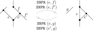
Figure 7: Redundancies due to the creation of a triangle and the reticulation edges of a triangle with listed redundant SNPR operations.

Proposition 3.10.

Let $N\in\mathcal{TC}_{n}$.

Then the number of non-trivial redundant SNPR operations of $\Theta_{\textup{{SNPR}}}^{\mathcal{TC}}(N)$ minus the number of redundancy sets of non-trivial SNPR operations of $\Theta_{\textup{{SNPR}}}^{\mathcal{TC}}(N)$ is

$$2n(2+t_{3})+r(2+t_{3})+4r_{1}-2r_{3}-8t_{3}+t_{3}^{*}+3d_{4}+t_{4}-8-\sum\limits_{e\in E_{\bar{t_{3}}}}\delta_{T}(e)\text{.}$$

Proof 3.11.

Let $\theta=(e,f)\in\Theta_{\textup{{SNPR}}}^{\mathcal{TC}}(N)$ such that $\theta(N)=N^{\prime}\neq N$. Let $e=(u,v),f=(x,y)$.

The operations we want to count are those that we want to discard when counting neighbours. To count all the operations we can discard, we go through the sources of redundancy one by one and determine the sizes of the corresponding redundancy sets. In order to find all sources, the idea of this proof is to consider when and where $\theta$ can be redundant with other operations. To cope with all possibilities, we fix a reticulation including a cycle for which this reticulation is the lowest vertex (i.e. descendant of all other vertices on the cycle). Then, when applying $\theta$, it can be distinguished whether the size of this cycle gets decreased, increased, or whether only the order of edges with start vertex on the cycle gets altered. Therefore in the following case distinction, we denote the change from a cycle of size $c$ to size $c^{\prime}$ by $[c\to c^{\prime}]$. Note that there can be no cycle of size 1 or 2. A cycle size of 0 denotes either no cycle, i.e. a tree, or that no cycle is under consideration or of any influence to redundancies of $\theta$.

One source of redundancy that we already identified are NNI operations with a pure inner tree edge as axis. A phylogenetic network has $n+r_{1}-2$ pure inner tree edges (all edges minus any incident to reticulations, leaves or the root) each inducing two NNI operations. However, if the axis is part of an $r_{3}$ structure, then one of the possible NNI for this axis is not tree-child respecting. Also, if it is part of a triangle, the operation is either trivial or not tree-child respecting. There are thus $2(n+r_{1}-2)-r_{3}-t_{3}$ NNI operations of interest, each with an SNPR redundancy set of size three. Therefore, we discard the following many non-trivial tree-child-respecting SNPR operations:

$$4n+4r_{1}-2r_{3}-2t_{3}-8$$ (4)

We freely use Proposition 1 throughout the remainder of this proof.

$[0\to 0]$

If no cycle is involved, the part where the SNPR operations make changes is tree-like and there are thus only tree edges. It follows thus from Lemma 3.7 that the redundancy comes from an NNI operation. Hence, these redundancies are covered by Equation 4.

$[3\to 3]$

A triangle with fixed reticulation has only one shape and thus can not be transformed into another one with a single SNPR operation.

In the following two cases, we will see redundancies due to the reticulation edges of triangles. We will count the SNPR operations we discard afterwards.

$[3\to 4]$

A triangle can be transformed into a cycle of size four either by pruning one of its edges and regrafting it to an edge outside of the triangle, thus including this edge as third outgoing edge or by regrafting an edge from outside to the triangle. We will see that considering only the latter case will also cover all of the former case.

Let the edge $e=(u,v)$ have distance at least two to the triangle and let $f=(x,y)$ be an edge of the triangle. Assuming $e$ has distance greater than two, it is clear (for example with the analysis of Lemma 3.8) that there can only be a redundancy, if $e$ is the reticulation edge of another triangle and $f$ the top side of the triangle. However, no SNPR operation pruning an edge of the fixed triangle or incident to it can be redundant to this operation and thus any redundancy would be accredited to the other triangle. Therefore, assuming now that $e$ has distance two to the triangle, the following cases can be distinguished.

(i) $u$ is parent of triangle,

$f$ is long side of triangle. Requiring that $e$ is a tree edge, the triangle gets transformed into a diamond. Using the analysis of Lemma 3.8 with $y$ and $v$ as siblings in $N^{\prime}$ yields that there are four redundant SNPR operations, as illustrated by Figure 8. Three SNPR operations can be associated to the NNI operation $(e,c,f)$ where $c$ is the incoming edge of the triangle. Also, pruning one of the two reticulation edges of the triangle and regrafting it to $e$ is redundant to doing the same with the other. We note that the SNPR operation $(f,e)$ corresponds to both redundancies.

(ii) $u$ is sibling of reticulation of triangle,

$f$ is long side of triangle. Requiring that both $e$ and its sibling edge are tree edges (and thus that the triangle is a tree-branching triangle), this transforms the triangle again into a diamond (see again Figure 8). This time the analysis, again with $y$ and $v$ as siblings, yields a redundancy set of size two, namely regrafting $e$ and its sibling edge $e^{\prime}$ to $f$.

This means that each tree-branching triangle of $N$ induces a redundancy set of size two. We thus discard one SNPR operation per such triangle:

$$t_{3}^{*}$$ (5)

(iii) $u$ is parent of triangle,

$f$ is top side of triangle. Without a requirement on $e$, this transforms the triangle into a trapezoid (see Figure 9). Like in (i), the analysis with $v$ being uncle of $y$, yields again an NNI operation redundancy with an overlap of a triangle reticulation edges redundancy. Furthermore, this can coincide with a transformation of another triangle into a trapezoid of the next case.

(iv) $u$ is sibling of reticulation of triangle,

$f$ is top side of triangle. This requires that the sibling edge of $e$ is a tree edge and transforms the triangle into a trapezoid (see again Figure 9). The analysis yields the same as in the previous case. If the sibling edge of $e$ is not a tree edge, we would have an $r_{3}$ structure and $N^{\prime}$ would not be tree child.

Furthermore, if $e$ is a tree edge, the case is equivalent to $f$ being the bottom side of the triangle.

(v) $u$ is parent of triangle,

$f$ is bottom side of triangle. The analysis yields that there is no redundancy of SNPR operations here.

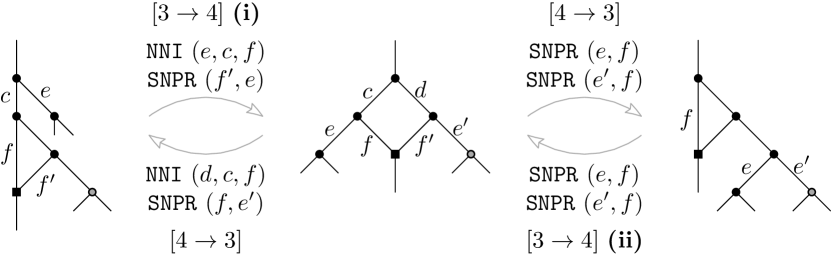
Figure 8: Transformation of triangles into diamonds and vice versa with listed redundancies, covering parts of the cases $[3\to 4]$ and $[4\to 3]$.

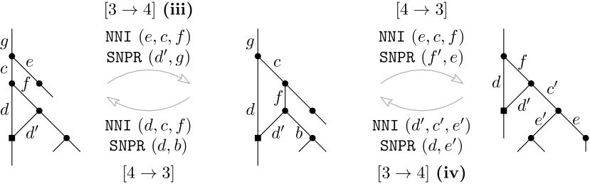
Figure 9: Transformation of triangles into trapezoids and vice versa with listed redundancies, covering parts of the cases $[3\to 4]$ and $[4\to 3]$.

$[3\to c,c\geq 5]$

Since it is not possible to add two outgoing edges to a triangle by regrafting them to the triangle with a single SNPR operation, the size can only be increased by pruning an edge of the triangle and regrafting it to an edge $f$ at the desired distance. This yields the same neighbour for the two reticulation edges, but different cycles for the top side of the triangle and one of its reticulation edges.

From the last two cases, we know that two SNPR operations $\theta$ and $\theta^{\prime}$ that prune the two different reticulation edges of a triangle and regraft it to the same edge are always redundant. In cases, where $\theta$ and $\theta^{\prime}$ are also redundant to SNPR operations corresponding to an NNI operation, either $\theta$ or $\theta^{\prime}$ also corresponds to that NNI operation. In any case, without loss of generality, we can discard all (non-trivial) SNPR operations that prune an edge $e\in E_{\bar{t_{3}}}$, i.e the bottom side of a triangle:

$$2nt_{3}+rt_{3}-4t_{3}-\sum\limits_{e\in E_{\bar{t_{3}}}}\delta_{T}(e)$$ (6)

$[4\to 3]$

This is basically the analysis of $[3\to 4]$ backwards. See again Figures 8 and 9 for illustrations.

$[c\to 3,c\geq 5]$

To create a triangle with a specific reticulation, one way is to prune one of its reticulation edges and to regraft it to an edge incident to the other reticulation edge. This is the reverse of $[3\to c]$ and yields two redundancy sets of size two.

The second possibility is to to prune the parent edge of one of the reticulation edges and regraft it to the other reticulation edge. Again, as seen in $[3\to c]$, this is not redundant to the other way or other operations.

The last two cases covered the creation of triangles. With Equation 5 we accounted for redundancies from a tree-branching triangle to a diamond. With Equation 7 we do the reverse:

$$d_{4}$$ (7)

Furthermore, as the reverse of Equation 6, each reticulation edge that is not part of a triangle corresponds to two redundant SNPR operations. In the case that a four cycle is created, this can coincide with a redundancy due to an NNI operation. Like before, we can discard one of the two operations:

$$2r-2t_{3}$$ (8)

$[4\to 4]$

To change a cycle of size four into another cycle of size four, one can either change the order of the outgoing edges of a trapezoid, which is then equivalent to Case $[0\to 0]$, or transform a trapezoid into a diamond or vice versa (see Figure 10). Applying Lemma 3.8 for any of the directions with two appropriate vertices yields redundancy sets of size four. We see that three edges correspond to an NNI operation. We have thus already counted a neighbour and can discard the fourth SNPR operation. We note that there are two different transformations from a diamond to a trapezoid distinguished by the order of the resulting trapezoid’s outgoing edges. Hence, we discard the following many SNPR operations:

$$2d_{4}+t_{4}$$ (9)

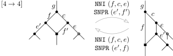
Figure 10: Transformation of diamonds into $t_{4}$ trapezoids and vice versa with listed redundancies, illustrating the case $[4\to 4]$.

$[c\to c+1,c\geq 4]$

Adding a branch to a cycle of size at least four, and thus increasing its size by one, is, by using Lemma 3.8, only possible if the operations correspond to an NNI operation.

$[c\to c+x,c\geq 4,x\geq 2]$

Unlike in the case $[3\to 5]$ there is obviously no redundancy of any edges of the cycle anymore.

$[c+1\to c,c\geq 4]$

This is the reverse of $[c\to c+1]$ and there are thus only redundancies due to an NNI operation.

$[c+x\to c,c\geq 4,x\geq 2]$

As the reverse of the case $[c+x\to c]$, there are no redundancy in this case.

We have now covered all cases of transformations of a cycle into another one. We have further identified the different sources of redundancies and discarded non-trivial tree-child-respecting SNPR operations accordingly. Adding Equations 4, 5, 6, 7, 8, 8 and 9 together, the statement follows.

The unit SNPR tree-child neighbourhood.

The unit SNPR tree-child neighbourhood of $N$ is determined by the number of tree-child-respecting SNPR operations on $N$ (Lemma 3.3), from which trivial operations are subtracted (Lemma 3.5) and operations that yield redundant neighbours are discarded (Proposition 3.10).

Theorem 3.12.

Let $N\in\mathcal{TC}_{n},n\geq 2$.

Then the unit SNPR tree-child neighbourhood $U_{\textup{{SNPR}}}^{\mathcal{TC}}(N)$ of $N$ has size

$$\begin{split}\lvert U_{\textup{{SNPR}}}^{\mathcal{TC}}(N)\rvert&=4n^{2}+10nr-2n(r_{2}+r_{3}+t_{3})-14n+2r^{2}-r(3r_{2}+3r_{3}+t_{3})\\ &-11r-4r_{1}+4r_{2}+7r_{3}+5t_{3}-t_{3}^{*}-3d_{4}-t_{4}+14\\ &-\sum\limits_{e\in E_{T^{*}}}\delta(e)-\sum\limits_{e\in E_{R}}\delta_{T}(e)+\sum\limits_{e\in E_{\bar{t_{3}}}}\delta_{T}(e)\text{.}\end{split}$$

Table 1 lists the values for the parameters of the tree-child network $N$ from Figure 3. Applying these values to Theorem 3.12 we get that $N$ has $7$ different SNPR tree-child neighbours, as depicted in Figure 3.

parameter	description	in $N$
$n$	# leaves	3
$r$	# reticulations	1
$r_{1}$	# reticulations with leaf as child	1
$r_{2}$	# $r_{2}$ structures	0
$r_{3}$	# $r_{3}$ structures	0
$t_{3}$	# triangles	0
$t_{3}^{*}$	# tree-branching triangles	0
$d_{4}$	# diamonds	0
$t_{4}$	# $t_{4}$ trapezoids	1
$\sum_{e\in E_{T^{*}}}\delta(e)$	# descendant edges of pure non-critical tree edges	13
$\sum_{e\in E_{R}}\delta_{T}(e)$	# descendant tree edges of reticulation edges	2
$\sum_{e\in E_{\bar{t_{3}}}}\delta_{T}(e)$	# descendant tree edges of triangle bottom sides	0

Table 1: Parameters for the network $N$ from Figure 3, which has a unit SNPR tree-child neighbourhood of size $7$.

If $N$ is a phylogenetic tree, it has of course zero reticulations and no special structures. We thus get the following formula for phylogenetic trees.

Corollary 3.13.

Let $T=(V,E)\in\mathcal{T}_{n}$.

Then the unit SNPR tree neighbourhood $U_{\textup{{SNPR}}}^{\mathcal{T}}(T)$ of $T$ has size

$$\lvert U_{\textup{{SNPR}}}^{\mathcal{T}}(T)\rvert=4n^{2}-14n+14-\sum\limits_{e\in E}\delta(e)\text{.}$$

Accounting for the fact that we count descendants of edges and not ancestors of vertices, this formula equals the result by Song [21].

The unit SNPR$+$ and SNPR$-$ tree-child neighbourhood.

We now consider SNPR$+$ and SNPR$-$ operations and count again first the number of such operations. For this, let $E_{PS}$ denote the set of edges that are pure tree edges with a sibling pure tree edge.

Lemma 3.14.

Let $N\in\mathcal{TC}_{n}$ with $n\geq 2$.

Then

$$\begin{split}\lvert\Theta_{\textup{{SNPR$+$}}}^{\mathcal{TC}}(N)\rvert&=4n^{2}-2nr-8n-2r^{2}+2r+4-\sum\limits_{e\in E_{PS}}\delta_{T}(e)\text{, and}\\ \lvert\Theta_{\textup{{SNPR$-$}}}^{\mathcal{TC}}(N)\rvert&=2r\text{.}\end{split}$$

Proof 3.15.

For an SNPR$+$ operation $(e,f)$, which adds an edge from $f$ to $e$, for $(e,f)(N)$ to be tree child, $e$ has to be a pure tree edge with a sibling pure tree edge. This implies that $e\neq e_{\rho}$ and that $e$ can not be incident to a reticulation or sibling edge of a reticulation edge. Otherwise, if $e$ would be incident to a reticulation, this would yield a pure reticulation edge, and if $e$ would be the sibling edge of a reticulation edge, this would yield a vertex with two reticulations as children. In either case $(e,f)(N)$ would not be tree child. Thus every reticulation induces a set of five edges, consisting of the three edges incident to it and their two sibling edges. Since $N\in\mathcal{TC}_{n}$, clearly these sets are disjoint for every pair of reticulations of $N$. There are thus $m-5r-1$ choices for $e$.

Next, by the definition of an SNPR$+$ operation, the edge $f$ can not be a descendant of $e$. Furthermore, $f$ can not be a reticulation edge or $e$. Otherwise, if $f$ would be a reticulation edge, this would yield a vertex with two reticulations as children, and if $f=e$, the operation would create a parallel edge. In either case $(e,f)(N)$ would not be tree child. Clearly any other choice of $f$ is fine. For any feasible choice of $e$, there are thus $m-2r-1-\delta_{T}(e)$ choices of $f$. With the $\delta_{T}(e)$ summing up to $\sum_{e\in E_{PS}}\delta_{T}(e)$ over all choices of $e$ and $(m-5r-1)(m-2r-1)=4n^{2}-2nr-8n-2r^{2}+2r+4$ the first statement follows.

Concerning $\Theta_{\textup{{SNPR$-$}}}^{\mathcal{TC}}(N)$, it is easy to see that removing any reticulation edge of a tree-child network yields again a tree-child network. There are thus $2r$ tree-child respecting SNPR$-$ operations on $N$.

Note that SNPR$+$ and SNPR$-$ operations are never trivial, since they change the number of reticulations. However, for both of these types of operations redundancies might exist. Like for most SNPR redundancies, these redundancies are equivalent to NNI$+$ and NNI$-$ operations, as the proof of the following proposition shows.

Proposition 3.16.

Let $N\in\mathcal{TC}_{n}$ with $n\geq 2$.

Then the unit SNPR$+$ tree-child neighbourhood $U_{\textup{{SNPR$+$}}}^{\mathcal{TC}}$ of $N$ has size

$$\lvert U_{\textup{{SNPR$+$}}}^{\mathcal{TC}}(N)\rvert=4n^{2}-2nr-10n-2r^{2}+4r+6-\sum\limits_{e\in E_{PS}}\delta_{T}(e)\text{,}$$

and the unit SNPR$-$ tree-child neighbourhood $U_{\textup{{SNPR$-$}}}^{\mathcal{TC}}$ of $N$ has size

$$\lvert U_{\textup{{SNPR$-$}}}^{\mathcal{TC}}(N)\rvert=2r-t_{3}\text{.}$$

Proof 3.17.

This proof uses the concept of the proof of Proposition 3.10. For the first part, we assume that the considered SNPR$+$ operations are tree-child respecting.

$[0\to 3]$

Let $f=(u,v)$ be a tree edge with $v$ having two outgoing pure tree edges $e=(v,w)$ and $e^{\prime}=(v,y)$. Then a reticulation and a triangle can be added by the SNPR$+$ operation $(e,f)$, which adds an edge from $f$ to $e$. This is however redundant to the SNPR$+$ operation $(e,e^{\prime})$. It follows by the uniqueness of $e$ that there are no further redundant SNPR$+$ operations. Furthermore, these operations are redundant to the NNI$+$ operation $(e,e^{\prime})$.

$[0\to c,c\geq 4]$

Similar to $[0\to 3]$, the edge $e$ that gets subdivided for the new reticulation is unique. However, for a new cycle of size at least 4, there are no two edges that can be chosen interchangeably to be subdivided for the source of the new reticulation edge to yield the same network $N^{\prime}$.

There are $n-r-1$ pairs of siblings of pure tree edges in $N$. To account for redundancy, we can thus discard $2(n-r-1)$ SNPR$+$ operations. The first part follows then from Lemma 3.14.

$[3\to 0]$

If a triangle gets removed, removing one of the reticulation edge of the triangle is redundant to removing the other. Since no reticulations are isomorphic in $N$, there can be no further reticulation edges in $N$ that if removed would yield the same network. These SNPR$-$ operations are thus equivalent to an NNI$-$ operation of the respective triangle.

$[c\to 0,c\geq 4]$

The reticulation edges of a cycle of size at least four are neither isomorphic nor can they change roles like in triangles. Thus removing a reticulation edge can not be redundant to removing another of a cycle of size at least four.

There are $t_{3}$ many NNI$-$ operations in $N$. Discarding one SNPR$-$ operation per triangle, the second part follows again from Lemma 3.14.

We can again consider the tree-child network $N$ from Figure 3. Since $N$ has one reticulation, but no triangles, $N$ has two SNPR$-$ neighbours. Using Table 1 and the fact that $\sum_{e\in E_{PS}}\delta_{T}(e)=2$, we get that $N$ has $6$ SNPR$+$ tree-child neighbours.

The unit SNPR tree-child neighbourhood.

To obtain the total size of the SNPR tree-child neighbourhood of a tree-child network $N$ we can now add together the sizes of the SNPR, SNPR$+$ and SNPR$-$ neighbourhoods (Theorems 3.12 and 3.16).

Theorem 3.18.

Let $N\in\mathcal{TC}_{n}$ with $n\geq 2$.

Then the unit SNPR tree-child neighbourhood $U_{\textup{SNPR}}^{\mathcal{TC}}$ of $N$ has size

$$\begin{split}\lvert U_{\textup{SNPR}}^{\mathcal{TC}}(N)\rvert&=8n^{2}+8nr-2n(r_{2}+r_{3}+t_{3})-24n-r(3r_{2}+3r_{3}+t_{3})-5r\\ &-4r_{1}+4r_{2}+7r_{3}+4t_{3}-t_{3}^{*}-3d_{4}-t_{4}+20\\ &-\sum\limits_{e\in E_{T^{*}}}\delta(e)-\sum\limits_{e\in E_{R}}\delta_{T}(e)-\sum\limits_{e\in E_{PS}}\delta_{T}(e)+\sum\limits_{e\in E_{\bar{t_{3}}}}\delta_{T}(e)\text{.}\end{split}$$

We conclude this section with the comment that, since each parameter and sum can be computed in $\mathcal{O}(n)$ time ($r,m\in\mathcal{O}(n)$), the unit SNPR tree-child neighbourhood size of a tree-child network $N$ can be computed in linear time $\mathcal{O}(n)$.

4 Minimal and maximal neighbourhoods

The formula for the unit SNPR tree-child neighbourhood of a tree-child network depends on a lot of parameters. It is therefore of interest to see how small and big a neighbourhood can get in terms of $n$.

Proposition 4.1.

Let $n\geq 2$. Then

$$\begin{split}n-1\leq&\min_{N\in\mathcal{TC}_{n}}\{\lvert U_{\textup{SNPR}}^{\mathcal{TC}}(N)\rvert\}\leq\frac{3}{2}n^{2}-\frac{7}{2}n+2\text{, and}\\ 8n^{2}-\mathcal{O}(n\log_{2}n)\leq&\max_{N\in\mathcal{TC}_{n}}\{\lvert U_{\textup{SNPR}}^{\mathcal{TC}}(N)\rvert\}<16n^{2}-38n+26\text{.}\end{split}$$

Proof 4.2.

We first establish a lower bound for the minimal neighbourhood size of a tree-child network. Let $N\in\mathcal{TC}_{n}$ with $n\geq 2$ and $r$ reticulations. By Proposition 3.16, we have that $\lvert U_{\textup{{SNPR$-$}}}^{\mathcal{TC}}(N)\rvert=2r-t_{3}$. Each reticulation gives rise to two different SNPR$-$ operations with redundancy sets of size at most two. Furthermore, a reticulation edge can be added from the root edge $e_{\rho}$ to every other pure tree edge that is not sibling edge of a reticulation edge. There are $2n-2r-2$ such edges. Note that $t_{3}\leq n-1$. There are thus at least $2n-2r-2+2r-t_{3}=2n-t_{3}-2\geq n-1$ SNPR tree-child neighbours of $N$. This is sharp for a tree-child network with $n=2$ and $r=1$.

Next, we look at an upper bound for the minimal neighbourhood size of a tree-child network. For this we consider a family of tree-child networks, where each has a relative small neighbourhood. Let $N_{r}\in\mathcal{TC}_{n},n\geq 2$ be a chain of $r$ triangles, where one triangle is child of the triangle above it in the chain, like $N_{4}$ in Figure 11. Since $N_{r}$ has $n-1$ reticulations, $N_{r}$ has no SNPR$+$ neighbours. Removing a reticulation edge from one of the triangles corresponds to one of $r=n-1$ different SNPR$-$ neighbours of $N_{r}$. Concerning SNPR operations, the only prunable non-critical edges are the long sides of the triangles (and the bottom sides, which however behave redundantly and are thus ignored). Since these are reticulation edges they can, when pruned, only be regrafted to tree edges that are not their descendants. For the long side of the triangle closest to the root three such edges exist, which however correspond to trivial operations. For the long side of the triangle below six such edges exist, of which again three yield trivial operation. Thus, in total there are

$$3+6+9+12+\ldots+(n-2)3=\sum_{i=1}^{n-2}3i=\frac{3}{2}(n-2)(n-1)=\frac{3}{2}n^{2}-\frac{9}{2}n+3$$

SNPR neighbours. All together, $N_{r}$ has $\frac{3}{2}n^{2}-\frac{7}{2}n+2$ SNPR neighbours.

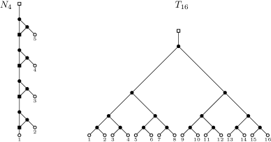
Figure 11: Tree-child networks with small and big neighbourhoods: The tree-child network $N_{4}$ has $\frac{3}{2}5^{2}-\frac{7}{2}5+2=22$ SNPR neighbours. The balanced tree $T_{16}$ has at least $8\cdot 16^{2}-4\cdot 16\log_{2}16-18\cdot 16+14=1518$ SNPR neighbours.

For a lower bound of the maximal SNPR tree-child neighbourhood size of a tree-child network, we consider the balanced tree $T_{n}$ on $n$ leaves, as illustrated by $T_{16}$ in Figure 11. The formula for the SNPR neighbourhood (Theorem 3.18) is then

$$8n^{2}-24n+20-\sum_{e\in E}\delta(e)-\sum_{e\in E_{PS}}\delta_{T}(e)\text{.}$$

For simplicity, we now assume that $n=2^{k}$ with $k\geq 1$. Then, for the first sum we have

$$\sum_{e\in E}\delta(e)=\sum_{i=1}^{\log_{2}n}i2^{i}=2n\log_{2}n-2n+2\text{.}$$

The second sum only differs from the first by the fact that the root edge $e_{\rho}$ is not in $E_{PS}$ and thus

$$\sum_{e\in E_{PS}}\delta_{T}(e)=2n\log_{2}n-2n+2-\delta(e_{\rho})=2n\log_{2}n-4n+4\text{.}$$

In total this yields that, for $n=2^{k}$, $T_{n}$ has $8n^{2}-4n\log_{2}n-18n+14$ SNPR neighbours. With no restriction on $n$, the tree $T_{n}$ has at least $8n^{2}-\mathcal{O}(n\log_{2}n)$ SNPR neighbours.

For an upper bound of the maximal SNPR neighbourhood size, we estimate bounds for the various parameters. We thus assume that the parameters $r_{1},r_{2},r_{3},t_{3},d_{4}$, and $t_{4}$ are zero. Concerning the sums $-\sum_{e\in E_{T^{*}}}\delta(e)-\sum_{e\in E_{R}}\delta_{T}(e)-\sum_{e\in E_{PS}}\delta_{T}(e)+\sum_{e\in E_{\bar{b}_{3}}}\delta_{T}(e)$ of the SNPR neighbourhood formula, we observe that the first and third sum are at best zero, that the second sum is at best $2r$ and that the last sum is at best half of the second. The sums account therefore only for $-r$ in our estimate. Assuming that $r=n-1$ and thus maximal, we get that for any tree-child network $N$ the unit SNPR tree-child neighbourhood has size at most $16n^{2}-38n+26$.

5 Discussion and outlook

In this paper, we have presented formulas for the unit SNPR tree-child neighbourhood size of tree-child networks. We have shown that the neighbourhood size does not only depend on the number of leaves and reticulations, but also on the shape of the network. In the formulas the shape is represented by the occurrences of certain structures, like triangles and diamonds, and the number of descendant edges of certain edge sets. The size of the SNPR$-$ neighbourhood is at most $n-1$, because the number of reticulations in a tree-child network is at most $n-1$ [6, Proposition 1]. On the other hand, the SNPR and SNPR$+$ neighbourhoods can both have a quadratic size in terms of $n$. We presented further bounds on the minimal and maximal neighbourhood size.

The main tool in our proofs of redundancy of operations was Proposition 1, which states every tree-child network has exactly one automorphism that fixes its leaf set. This allowed us to pinpoint redundancies to some simple structures. Our methodology can be applied to other network classes, especially subclasses of tree-child networks. For example, normal networks are tree-child networks that do not contain both an edge $(u,v)$ and a path from $u$ to $v$ that consists of at least two edges. Vertices and edges are thus also unique in normal networks and, moreover, they do not contain triangles or trapezoids. While this simplifies counting SNPR redundancies, it comes at the cost that counting all normal-respecting SNPR operations get harder. Another class that is suitable for our methodology is the class of level-1 networks. A phylogenetic network is level-1 if each of its biconnected components contains at most one reticulation. A level-1 network without parallel edges is thus also a tree-child network. The size of the unit SNPR neighbourhood for normal and level-1 networks can be found in the author’s thesis [18].

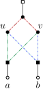
Figure 12: A reticulation-visible (and tree-based) network with non-unique vertices and edges. The vertices $u$ and $v$ are isomorphic and so are the three groups of edges in same colour and style.

Finding a formula for the unit SNPR neighbourhood is more complicated for the network classes of reticulation-visible and tree-based networks. A phylogenetic network is reticulation visible if every reticulation separates the root from at least one leaf [16]. Roughly speaking, a phylogenetic network is tree based if it is contains a phylogenetic tree on the same leaf set that covers all its vertices [10]. The class of tree-child networks is known to be a subclass of both the classes of reticulation-visible and tree-based networks [10]. However, Figure 12 shows a reticulation-visible (and thus also tree-based) network with only two leaves and two reticulations, where two isomorphic vertices and three pairs of isomorphic edges exist. More complicated phylogenetic networks with bigger sets of pairwise isomorphic vertices or edges can easily be found. Isomorphic edges in a phylogenetic network have the consequence that pruning one of them or regrafting to one of them is redundant to any of the others. Determining the size of a neighbourhood would thus require to identify and account for all equivalences. While we think that a recursive approach (similar to the work of Song [21, 22]) to count neighbours might still be possible, a closed formula is likely to require even more parameters.

The space of rooted phylogenetic networks under NNI has, in contrast to the unrooted case, not found much attention in the literature so far. We defined NNI operations for tree-child networks as a tool to count several redundancies. However, to consider the space itself and its properties could be of interest.

References

- [1] B. L. Allen and M. Steel. Subtree transfer operations and their induced metrics on evolutionary trees. Annals of Combinatorics, 5(1):1–15, 2001.
- [2] S. Baskowski, V. Moulton, A. Spillner, and T. Wu. Neighborhoods of trees in circular orderings. Bulletin of Mathematical Biology, 77(1):46–70, 2015.
- [3] M. Bordewich, S. Linz, and C. Semple. Lost in space? Generalising subtree prune and regraft to spaces of phylogenetic networks. Journal of Theoretical Biology, 423:1–12, 2017.
- [4] M. Bordewich and C. Semple. Determining phylogenetic networks from inter-taxa distances. Journal of Mathematical Biology, 73(2):283–303, 2016.
- [5] M. Bordewich, C. Semple, and N. Tokac. Constructing tree-child networks from distance matrices. Algorithmica, pages 1–20, 2017.
- [6] G. Cardona, F. Rossello, and G. Valiente. Comparison of tree-child phylogenetic networks. IEEE/ACM Trans. Comput. Biol. Bioinformatics, 6(4):552–569, Oct 2009.
- [7] P. Cordue, S. Linz, and C. Semple. Phylogenetic networks that display a tree twice. Bulletin of Mathematical Biology, 76(10):2664–2679, 2014.
- [8] J. V. de Jong, J. C. McLeod, and M. Steel. Neighborhoods of phylogenetic trees: Exact and asymptotic counts. SIAM Journal on Discrete Mathematics, 30(4):2265–2287, 2016.
- [9] A. Francis, K. T. Huber, V. Moulton, and T. Wu. Bounds for phylogenetic network space metrics. Journal of Mathematical Biology, 76(5):1229–1248, Apr 2018.
- [10] A. R. Francis and M. Steel. Which phylogenetic networks are merely trees with additional arcs? Systematic Biology, 64(5):768–777, 2015.
- [11] P. Gambette, V. Berry, and C. Paul. The structure of level-k phylogenetic networks. In G. Kucherov and E. Ukkonen, editors, Combinatorial Pattern Matching, pages 289–300. Springer Berlin Heidelberg, 2009.
- [12] P. Gambette, L. van Iersel, M. Jones, M. Lafond, F. Pardi, and C. Scornavacca. Rearrangement moves on rooted phylogenetic networks. PLOS Computational Biology, 13(8):1–21, Aug 2017.
- [13] K. T. Huber, S. Linz, V. Moulton, and T. Wu. Spaces of phylogenetic networks from generalized nearest-neighbor interchange operations. Journal of Mathematical Biology, 72(3):699–725, 2016.
- [14] K. T. Huber, V. Moulton, and T. Wu. Transforming phylogenetic networks: Moving beyond tree space. Journal of Theoretical Biology, 404:30–39, 2016.
- [15] P. J. Humphries and T. Wu. On the neighborhoods of trees. IEEE/ACM Transactions on Computational Biology and Bioinformatics, 10(3):721–728, May 2013.
- [16] D. H. Huson and T. H. Klöpper. Beyond galled trees - decomposition and computation of galled networks. In T. Speed and H. Huang, editors, Research in Computational Molecular Biology, pages 211–225. Springer Berlin Heidelberg, 2007.
- [17] R. Janssen, M. Jones, P. L. Erdős, L. van Iersel, and C. Scornavacca. Exploring the tiers of rooted phylogenetic network space using tail moves. Bulletin of Mathematical Biology, Jun 2018.
- [18] J. Klawitter. Spaces of phylogenetic networks. PhD thesis, University of Auckland, in preparation.
- [19] C. McDiarmid, C. Semple, and D. Welsh. Counting phylogenetic networks. Annals of Combinatorics, 19(1):205–224, 2015.
- [20] D. Robinson. Comparison of labeled trees with valency three. Journal of Combinatorial Theory, Series B, 11(2):105–119, 1971.
- [21] Y. S. Song. On the combinatorics of rooted binary phylogenetic trees. Annals of Combinatorics, 7(3):365–379, 2003.
- [22] Y. S. Song. Properties of subtree-prune-and-regraft operations on totally-ordered phylogenetic trees. Annals of Combinatorics, 10(1):147–163, 2006.
- [23] L. van Iersel, C. Semple, and M. Steel. Locating a tree in a phylogenetic network. Information Processing Letters, 110(23):1037–1043, 2010.
- [24] S. J. Willson. Unique determination of some homoplasies at hybridization events. Bulletin of Mathematical Biology, 69(5):1709–1725, Jul 2007.
- [25] S. J. Willson. Properties of normal phylogenetic networks. Bulletin of Mathematical Biology, 72(2):340–358, Feb 2010.