Construction of helices from Lucas and Fibonacci sequences

Abstract: By means of two complex-valued functions (depending on an integer parameter $P\geq 1$) we construct helices of integer ratio $R\geq 1$ related to the so-called Binet formulae for P-Lucas and P-Fibonacci sequences. Based on these functions a new map is defined and we show that its three-dimensional representation is also a helix. After proving that the lattice points of these later helix satisfy certain diophantine Pell’s equations we call it a Pell’s helix. We prove that for P-Fibonacci and Pell’s helices the respective ratio is an invariant, contrasting to the P-Lucas helices whose ratio depends on $P$. It is also shown that suitable linear combinations of certain complex-valued maps lead to new helices related to Lucas/Fibonacci/Pell numbers. Graphical examples are given in order to illustrate the underlying theory.

Keywords: Difference equation; helix; double helix; Binet formulae; Lucas sequence; Fibonacci sequence; diophantine Pell equation.

1 Introduction

In Section 2 we define two complex-valued functions $g$ and $h$ which are extended versions of the so-called sequence Binet formulae [7, 4], for two well-known families of sequences called P-Lucas and P-Fibonacci sequences, where $P\geq 1$ is an integer parameter (cf. (1) and (5)).

The maps $g$ and $h$ give rise to new complex-valued functions $\psi_{1}$, $\psi_{2}$ (see (14)) for which we show that their parametric representation in the three-dimensional space is a helix. We call these helices P-Lucas and P-Fibonacci helices, respectively.

In Proposition 2.1 we prove that all P-Fibonacci helices have ratio $R=1$, while the P-Lucas helices have ratio $R=P^{2}+4\geq 5$, all these helices having the same pitch $p=2$. The ratio invariance property of P-Fibonacci helices is fundamental to distinguish these helices from the P-Lucas ones.

The fact of the P-Fibonacci’s helices are ratio invariant, whose ratio $R=1$ is minimal relatively to the ratio of the P-Lucas helices, may bring a new point of view to a classic controversy on the so-called omnipresence of the “divine proportion” and other “metallic means” (see for instance [8] and bibliography therein) as well as to other issues relevant in the phyllotaxis area of research [1, 12].

In Section 3 we define another complex-valued function $\psi_{3}$ depending on $g$ and $h$. This map enables us to make a connection to certain Pell’s equations (see for instance [9], [3] Ch. 6.8).

The main results are propositions 3.1 and 3.2. In Proposition 3.1 we prove that the curves represented by $\psi_{3}$ are also ratio invariant helices ($R=4$). We name them P-Pell helices.

Of course, any expression involving suitable arrangements of the integer terms of Lucas/Fibonacci sequences (in the literature one can find a lot of such expressions) can be rewritten as a complex-valued map, say $\psi$, whose geometrical properties might be unveiled using a suitable parametrization of $\psi$. However, we restrict the scope only to three complex-valued functions $\psi_{1}$ $\psi_{2}$, defined in (14) (Lucas/Fibonacci) and $\psi_{3}$, defined in (28) (Pell) for which one can easily prove that they are representable as helices.

In Proposition 3.2 we define other maps $\psi_{4}$ to $\psi_{7}$, resulting from suitable linear combinations of $\psi_{1}$ to $\psi_{3}$, whose representative curve is also a helix. We conclude that by appropriate linear combinations of the referred complex-valued maps we are lead to innumerable other helices related to Lucas/Fibonacci/Pell numbers.

The examples given in Section 4 aim to illustrate that the representation of Lucas/Fibonnaci sequences by the complex maps $g$, $h$ and the subsequent maps $\psi_{1}$, $\psi_{2}$ and $\psi_{3}$, all provide tools to highlight geometrical aspects hidden either in their recursive definition or in the referred classical Binet formulae, expanding the findings for instance in [6], [11] and [5].

In examples 4.1-4.4 some Lucas/Fibonacci/Pell helices are displayed, from which a panoply of double helices can be constructed, as in Example 4.3, suggesting that Lucas/Fibonacci/Pell helices can perhaps find several applications within the scientific [13, 12], artistic [16] or industrial [14] frameworks.

We hope that this preliminary work, based on elementary mathematics, may be a source of inspiration in future studies. The approach, following the spirit of [10], seems to be a unifying setting to deal with geometrical and analytical aspects namely for difference equations.

2 Lucas-Fibonacci sequences

The family of P-Lucas sequences is defined by

$$\begin{array}[]{l}L_{0}=2\\ L_{1}=P\\ L_{n+2}=P\,L_{n+1}+L_{n},\qquad n=0,1,2,\ldots,\end{array}$$ (1)

where $P\geq 1$ is an integer. The characteristic polynomial associated to the difference equation (1) is

$$p(\lambda)=\lambda^{2}-P\,\lambda-1,$$ (2)

whose real roots are

$$\lambda_{1}=\displaystyle\frac{P+\sqrt{D}}{2}>0,\qquad\lambda_{2}=\displaystyle\frac{P-\sqrt{D}}{2}<0,\quad\mbox{with}\quad D=P^{2}+4\ .$$ (3)

The family of P-Fibonacci sequences is defined by same difference equation of the P-Lucas family with different initial values. Namely,

$$\begin{array}[]{l}F_{0}=0\\ F_{1}=1\\ F_{n+2}=P\,F_{n+1}+F_{n},\qquad n=0,1,2,\ldots\ .\end{array}$$ (4)

Both families share the same characteristic polynomial (2), and its roots satisfy the following properties which will play a crucial role later:

$$(i)\quad\lambda_{1}+\lambda_{2}=P,\quad(ii)\quad\lambda_{1}-\lambda_{2}=\sqrt{D},\quad(iii)\quad\lambda_{1}\,\lambda_{2}=-1\ .$$ (5)

Let us define two complex-valued functions modelling respectively the diference equations (1) and (4).

Definition 2.1.

Given an integer $P\geq 1$, we define the functions

$g,h:\mathbb{R}\mapsto\mathbb{C},$ by

$$\begin{array}[]{l}g(t)=\lambda_{1}^{t}+\lambda_{2}^{t},\qquad t\in\mathbb{R},\\ \\ h(t)=\displaystyle\frac{1}{\sqrt{D}}\left(\lambda_{1}^{t}-\lambda_{2}^{t}\right),\quad t\in\mathbb{R}\ .\end{array}$$ (6)

The functions $g$ and $h$ are called the (complex) representation of the P-Lucas sequence and P-Fibonacci sequence, respectively.

Note that by (5)-(iii) we have $\lambda_{2}=-1/\lambda_{1}<0$, and so

$$\lambda_{2}^{t}=\displaystyle\frac{1}{\lambda_{1}^{t}}\,\left(-1\right)^{t}\ .$$ (7)

Applying the Euler’s formula $e^{i\pi}=-1$, where $i=\sqrt{-1}$, we obtain

$$\lambda_{2}^{t}=\displaystyle\frac{e^{i\,\pi t}}{\lambda_{1}^{t}}=\displaystyle\frac{\cos(\pi\,t)+i\,\sin(\pi\,t)}{\lambda_{1}^{t}}\ .$$ (8)

By (8) one concludes that both $g$ and $h$, given by (6), can be seen as continuous complex-valued functions defined in $\mathbb{R}$.

In the sequel the (complex) representation of P-Lucas or Fibonacci sequences will be used to illustrate geometrical aspects hidden in their integer recursive definitions (1) or (4). When $P$ is assumed to be a given constant, P-Lucas or P-Fibonacci sequences will be simply called Lucas or Fibonacci sequences, respectively.

Restricting the real variable $t$ in (6) to the non-negative integers $\mathbb{Z}_{0}^{+}$, the values of $g$ and $h$ coincide with the well-known and widely used Binet formulae, respectively

$$\begin{array}[]{l}L_{n}=\displaystyle\frac{1}{2^{n}}\left(\displaystyle(P+\sqrt{D})^{n}+(P-\sqrt{D})^{n}\right),\quad n=0,1,\ldots\\ \\ F_{n}=\displaystyle\frac{1}{\sqrt{D}\,2^{n}}\left(\displaystyle(P+\sqrt{D})^{n}-(P-\sqrt{D})^{n}\right),\quad n=0,1,\ldots\ .\\ \end{array}$$ (9)

Given an integer $n$ and $D=P^{2}+4$ not a perfect square, the expressions in (9) show that we are dealing with rational, irrational and real numbers. Therefore formulae like (9) hardly highlight the geometrical aspects provided by their complex representation (6). Thus, the consideration of the independent real variable $t$, instead of $n$ used on the traditional Binet formulae [7, 4], enables to extend the functions $g$, $h$ in (6) to the geometrically rich set of complex numbers $\mathbb{C}$ (the geometric properties of standard complex-valued maps is comprehensively treated in [10]).

Let us begin by setting the notion of a three-dimensional curve and define what we mean by a P-Lucas or P-Fibonacci curve.

Definition 2.2.

(P-Lucas/Fibonacci curves)

Given a function $f:\mathbb{R}\mapsto\mathbb{C}$, we define the curve $\gamma_{f}:\mathbb{R}\mapsto\mathbb{R}^{3}$ by

$$\gamma(t)=\left(x(t),y(t),z(t)\right),$$

where

$$\left\{\begin{array}[]{l}x(t)={\cal R}e\,f(t)\\ y(t)={\cal I}m\,f(t)\\ z(t)=t,\hskip 113.81102ptt\in\mathbb{R}\ .\end{array}\right.$$ (10)

When $f=g$ or $f=h$, given in (6), the corresponding curve (10) will be called a P-Lucas or P-Fibonacci curve. In the case the value of $P$ is fixed we simply call the curve associated to $g$ (resp. $h$) Lucas curve (resp. Fibonacci curve).

In the particular instance such that

$$\left\{\begin{array}[]{l}x(t)={\cal R}e\,f(t)=R\,\cos(\pi\,t)\\ y(t)={\cal I}m\,f(t)=R\,\sin(\pi\,t)\\ z(t)=t\hskip 113.81102ptt\in\mathbb{R},\end{array}\right.$$ (11)

where $R>0$, the function $f$ is representable by the 3-dimensional helix of ratio $R$ and pitch $2$. Indeed, recall that the parametric equations

$$\left\{\begin{array}[]{l}x(\theta)=R\,\cos(\theta)\\ y(\theta)=R\,\sin(\theta)\\ z(\theta)=\displaystyle\frac{p}{2\,\pi}\,\theta,\hskip 85.35826pt\theta\geq 0\end{array}\right.$$ (12)

define the (rectangular) coordinates of the points of a helix with polar angle $\theta$, ratio $R>0$, and pitch $p>0$.

Helices like (11) and other helicoidal or spiral curves are widely present in the nature as well as in numerous mankind achievements (see for instance [2], [13], [16], [14]).

Remark 2.1.

If the parameter $t$ in (11) is an integer $k$ the component $z(k)=k$. Thus, in order that a point of the corresponding curve $\gamma_{f}$ be a lattice point (that is, a point with integer coordinates) we should have $x(k)$, $y(k)\in\mathbb{Z}$. Therefore, a point ${\cal P}_{j}$ belonging to the helix (11) is a lattice point if and only if $R\in\mathbb{Z}$, in which case

$${\cal P}_{j}=(\pm R,0,j),\qquad j\in\mathbb{Z}\ .$$ (13)

Note that in (11) we have considered the parameter $t\in\mathbb{R}$. In the examples given in Section 4 we restrict $t\in[t_{min},t_{max}]$, for given integers $t_{min}<t_{max}$.

The value $p$ in (12) represents the vertical displacement of a point in the helix after an angular increment of $2\,\pi$. The points of the helix lie in a cylinder with ratio $R$, the point $(0,0,0)$ being the origin of the coordinate system. Of course, for $\theta=0$, the point $(R,0,0)$ is on the helix. Consequently, a parametric curve given by $x(t)=R\cos(\pi t)$, $y(t)=R\sin(\pi t)$, $z(t)=t$, with $t_{min}\leq t\leq t_{max}$, represents the helix of polar ratio $R$ and pitch $2$, on a cylinder of radius $R$ and height $t_{max}-t_{min}$.

In the following Proposition 2.1 we discuss two maps $\psi_{1}$ and $\psi_{2}$ (depending on $g,h$ defined by (6)) which have the interesting property of being representable as helices.

Proposition 2.1.

Let $g$ and $h$ be respectively P-Lucas and P-Fibonacci curves. Consider the complex-valued functions

$$\begin{array}[]{l}\psi_{1}(t)=g^{2}(t)-g(t-1)\,g(t+1)\\ \psi_{2}(t)=h(t-1)\,h(t+1)-h^{2}(t),\,\qquad t\in\mathbb{R}\ .\\ \end{array}$$ (14)

(i) The curves of $\psi_{1}$ and $\psi_{2}$ are helices of polar angle $\theta=\pi\,t\,\,\mbox{(rad)}$ and (common) pitch $p=2$. We call the curve associated to $\psi_{1}(t)$ a P-Lucas helix and the one associated to $\psi_{2}(t)$ a P-Fibonacci.

(ii) For any integer $P\geq 1$ a P-Lucas helix and a P-Fibonacci one do not intersect.

(iii) For any integer $P\geq 1$, the P-Lucas sequence verify the equalities

$$L_{k}^{2}-L_{k-1}\,L_{k+1}=(P^{2}+4)\,(-1)^{k},\qquad k=0,1,2,\ldots$$ (15)

(iv) For any integer $P\geq 1$, the P-Fibonacci sequence verify the equalities

$$F_{k-1}\,F_{k+1}-F_{k}^{2}=(-1)^{k},\qquad k=0,1,2,\ldots$$ (16)

The ratio $R$ of the helices corresponding to the maps $\psi_{1}$ and $\psi_{2}$ is summarised in Table 1 as well as the ratio of a helix corresponding to a map $\psi_{3}$ to be introduced in Section 3.

Proof.

(i) From (6) and (5)-(iii), we have

$$\begin{array}[]{l}g^{2}(t)=\lambda_{1}^{2\,t}+\lambda_{2}^{2\,t}+2\,(\lambda_{1}\,\lambda_{2})^{t}=\lambda_{1}^{2\,t}+\lambda_{2}^{2\,t}+2\,(-1)^{t},\end{array}$$ (17)

and

$$g(t-1)\,g(t-2)=\lambda_{1}^{2\,t}+\lambda_{2}^{2\,t}+\lambda_{1}^{t-1}\,\lambda_{2}^{t-1}\,\left(\lambda_{2}^{2}+\lambda_{1}^{2}\right)\ .$$

Taking into account that $\lambda_{1}+\lambda_{2}=P$, $\lambda_{1}^{2}=P\,\lambda_{1}+1$ and $\lambda_{2}^{2}=P\,\lambda_{2}+1$, we get

$$\lambda_{1}^{2}+\lambda_{2}^{2}=P\,(\lambda_{1}+\lambda_{2})+2=P^{2}+2\ .$$

Since $\lambda_{1}\,\lambda_{2}=-1$, one obtains

$$\begin{array}[]{ll}g(t-1)\,g(t+1)&=\lambda_{1}^{2\,t}+\lambda_{2}^{2\,t}+(P^{2}+2)\,(-1)^{t-1}\\ &=\lambda_{1}^{2\,t}+\lambda_{2}^{2\,t}-(P^{2}+2)\,(-1)^{t}\ .\\ \end{array}$$ (18)

Thus, from (17) and (18), we have

$$\begin{array}[]{ll}\psi_{1}(t)&=g^{2}(t)-g(t-1)\,g(t+1)=(P^{2}+4)\,(-1)^{t}=D\,(-1)^{t}\\ &=D\,\left(\cos(\pi\,t)+i\,\sin(\pi\,t)\right),\qquad t\in\mathbb{R}\ .\end{array}$$ (19)

Therefore, the following curve

$$\left\{\begin{array}[]{l}x(t)={\cal R}e\,(\psi_{1}(t))=D\,\cos(\pi\,t)\\ y(t)={\cal I}m\,(\psi_{1}(t))=D\,\sin(\pi\,t)\\ z(t)=t,\hskip 170.71652pt\qquad t\in\mathbb{R}\end{array}\right.$$ (20)

is a helix of ratio $D=P^{2}+4$ and pitch $2$.

From (6) we have

$$D\,h^{2}(t)=\lambda_{1}^{2\,t}+\lambda_{2}^{2\,t}-2\,(\lambda_{1}\,\lambda_{2})^{t}=\lambda_{1}^{2\,t}+\lambda_{2}^{2\,t}-2\,(-1)^{t}$$ (21)

and

$$\begin{array}[]{ll}h(t-1)\,h(t+1)&=\displaystyle\frac{1}{D}\left(\lambda_{1}^{2\,t}+\lambda_{2}^{2\,t}-(\lambda_{1}\,\lambda_{2})^{t-1}\,(\lambda_{1}^{1}+\lambda_{2}^{2})\right)\\ \\ &=\displaystyle\frac{1}{D}\left(\lambda_{1}^{2\,t}+\lambda_{2}^{2\,t}-(P^{2}+2)\,(\lambda_{1}\,\lambda_{2})^{t-1}\right)\\ \\ &=\displaystyle\frac{1}{D}\left(\lambda_{1}^{2\,t}+\lambda_{2}^{2\,t}-(P^{2}+2)\,(-1)^{t-1}\right)\ .\\ \end{array}$$ (22)

Thus,

$$D\,\left(h(t-1)\,h(t+1)\right)=\lambda_{1}^{2\,t}+\lambda_{2}^{2\,t}+(P^{2}+2)\,(-1)^{t},$$

and so

$$D\,\left(h(t-1)\,h(t+1)-h^{2}(t)\right)=(P^{2}+4)\,(-1)^{t}=D\,(-1)^{t}\ .$$ (23)

That is,

$$\psi_{2}(t)=h(t-1)\,h(t+1)-h^{2}(t)=(-1)^{t}.$$ (24)

Using the same reasoning as before, the last equality shows that $\psi_{2}(t)$ can be written as a hélix with ratio $R=1$ and pitch $2$.

(ii) From (19) and (24) we conclude that

$$\psi_{1}=\,D\,\psi_{2}(t)=(P^{2}+4)\,\psi_{2}(t),\qquad t\in\mathbb{R}\ .$$ (25)

This means that a Lucas helix has a ratio that is $P^{2}+4$ greater than the ratio of the Fibonacci helix and the conclusion follows.

(iii) Follows from(19) for $t=0,1,2,\ldots\ .$

(iv) Follows from (24) for $t=0,1,2,\ldots\ .$ ∎

$$\begin{array}[]{|l|c|c| }\hline\cr\hskip 56.9055pt\mbox{Map}&R\,\,\mbox{(Ratio)}&\mbox{Helix name}\\ \hline\cr\psi_{1}(t)=g^{2}(t)-g(t-1)\,g(t+1)&P^{2}+4=D&\mbox{Lucas}\\ \hline\cr\psi_{2}(t)=h(t-1)\,h(t+1)-h^{2}(t)&1&\mbox{Fibonacci}\\ \hline\cr\psi_{3}(t)=g^{2}(t)-D\,h^{2}(t)&4&\mbox{Pell}\\ \hline\cr\end{array}$$

Table 1: Lucas/Fibonacci/Pell helices.

Remark 2.2.

The curves $\psi_{1}$ and $\psi_{2}$ defined in (14) are not the unique helices one can associate respectively to Lucas or Fibonacci sequences. For instance, from

$$g(2\,t)=\lambda_{1}^{2\,t}+\lambda_{2}^{2\,t}$$

and

$$g^{2}(t)=\lambda_{1}^{2\,t}+\lambda_{2}^{2\,t}+2\,(\lambda_{1}\,\lambda_{2})^{t}$$

we get

$$g(2\,t)-g^{2}(t)=-2\,(\lambda_{1}\,\lambda_{2})^{t}=2\,(-1)^{t}$$

and so

$${\cal L}(t)=g(2\,t)-g^{2}(t),$$ (26)

is a map representable as a helix (with ratio $R=2$) also associated to P-Lucas sequences.

Also, from (26) we get

$$L_{k}^{2}-L_{2\,k}=2\,(-1)^{k},\qquad k\in\mathbb{Z}$$ (27)

which is an extension of a well known relationship among terms of P-Lucas sequences ([3], p. 421, Proposition 6.8.1). However, in this preliminary work, we will not discuss further matters related to the map ${\cal L}$ given in (26) as well as other elaborations on the referred unicity issue.

New helices associated to the maps $\Psi_{1}$ and $\Psi_{2}$ will be defined in the next section.

3 Some helices related to diophantine equations of Pell

The next definition characterizes a certain helix which we name Pell’s helix due to its connection to two famous quadratic diophantine equations, namely $u^{2}-b\,v^{2}=4$ and $u^{2}-b\,v^{2}=-4$, where $b>0$ is a no perfect square integer and $u,v$ are integers (for the Pell-Fermat equation $u^{2}-b\,v^{2}=N$ see for instance [3], p. 354).

Consider the complex-valued function

$$\psi_{3}(t)=g^{2}(t)-D\,h^{2}(t),\qquad t\in\mathbb{R}\ .$$ (28)

As shown in Proposition 3.1 the function $\psi_{3}$ can be written as a helix of ratio $R=4$.

Definition 3.1.

A Pell’s helix (of ratio 4), is a helix parametrized by

$$\begin{array}[]{l}x(t)=4\,\cos(\pi\,t)\\ y(t)=4\,\sin(\pi\,t)\\ z(t)=t,\qquad\qquad t\in\mathbb{R}\ .\end{array}$$ (29)

.

Proposition 3.1.

Let $L_{k}$ and $F_{k}$ be the $k$-th terms of the sequences given in (9) and $\psi_{3}$ as in (28).

(i) The function $\psi_{3}$ can be written as Pell’s helix (29).

(ii) For $j$ integer, the following points ${\cal P}$ and ${\cal Q}$ are the only lattice points for the Pell’s helix (29):

$$\begin{array}[]{ll}{\cal P}_{j}=(4,0,j)&\mbox{for}\,\,j\,\,\mbox{even}\\ {\cal Q}_{j}=(-4,0,j)&\mbox{for}\,\,j\,\,\mbox{odd}\ .\\ \end{array}$$ (30)

(iii) The point $(L_{k},F_{k})$ satisfies respectively the diophantine equation $x^{2}-D\,y^{2}=4$ for $k$ even, and $x^{2}-D\,y^{2}=-4$ for $k$ odd.

Proof.

(i) From (17) and (21) we have

$$g^{2}(t)-D\,h^{2}(t)=4\,(-1)^{t},$$ (31)

and so the function $\psi_{3}$ can be written as the helix given by (29).

(ii) We have here a particular case of the curve in (11) with $R=4$ or $R=-4$ (see remark 2.1). So the lattice points corresponding to (13) are giving by (30).

(iii) For $t\in\mathbb{Z}$ the numbers $g(t)$, $D$ and $h(t)$ are integers. When $t$ is even, say $t=2\,k$ with $k\in\mathbb{Z}$, let $x=g(t)$, $y=h(t)$. By (31) we get $x^{2}-D\,y^{2}=4$. When $t$ is odd the same reasoning leads to $x^{2}-D\,y^{2}=-4$. ∎

Considering the maps given in Table 1 one concludes immediately that a suitable linear combination of $\psi_{1}$ to $\psi_{3}$ leads to new maps – denoted by $\psi_{4}$ to $\psi_{7}$ in Table 2 – which are also representable by helices, whose ratio $R_{m}$ is given in the second column of that table. Translating the tabulated maps by its expressions in terms of the maps $g$ and $h$, by direct computation from the definitions given for the maps $\psi_{m}$, for $m=4$ to $m=7$, immediately one justifies the following proposition and so we omit its proof. Of course other helices, related to P-Lucas/Fibonacci/Pell sequences, having ratio congruent to $0,1,2,\ldots,P^{2}+3$ $\pmod{D}$, could also be defined by means of a convenient linear combination of $\psi_{1},\psi_{2}$ and $\psi_{3}$.

$$\begin{array}[]{ |l |c| c |}\hline\cr\hskip 56.9055pt\mbox{Map}&R_{m}\,\,\mbox{(Ratio)}&\mbox{Connection}\\ \hline\cr\psi_{4}(t)=\psi_{1}(t)-(D-1)\,\psi_{2}(t)&1&\mbox{Fibonacci\--Lucas}\\ \hline\cr\psi_{5}(t)=\psi_{3}(t)-2\,\psi_{2}(t)&2&\mbox{Pell\--Fibonacci}\\ \hline\cr\psi_{6}(t)=\psi_{3}(t)-\psi_{2}(t)&3&\mbox{Pell\--Fibonacci}\\ \hline\cr\psi_{7}(t)=2D\,\psi_{2}(t)-\psi_{1}(t)&D=P^{2}+4&\mbox{Fibonacci--Lucas}\\ \hline\cr\end{array}$$

Table 2: Maps $\psi_{4}$ to $\psi_{7}$.

Proposition 3.2.

The following complex-valued maps $\psi_{4}$ to $\psi_{7}$, expressed in terms of $g$, $h$ given in (6), are all representable by helices whose ratio $R_{m}$ is summarized in Table 2.

$$\begin{array}[]{l}\psi_{4}(t)=\psi_{1}(t)-(D-1)\,\psi_{2}(t)=\\ \hskip 28.45274pt=g^{2}(t)-g(t-1)\,g(t+1)-(P^{2}+3)\,\left(h(t-1)\,h(t+1)-h^{2}(t)\right)=\\ \hskip 28.45274pt=(-1)^{t},\\ \\ \psi_{5}(t)=\psi_{3}(t)-2\,\psi_{2}(t)=\\ \hskip 28.45274pt=g^{2}(t)-(P^{2}+2)\,h^{2}(t)-2\,h(t-1)\,h(t+1)=2\,(-1)^{t},\\ \\ \psi_{6}(t)=\psi_{3}(t)-2\,\psi_{2}(t)=\\ \hskip 28.45274pt=g^{2}(t)-(P^{2}+4)\,h^{2}(t)-h(t-1)\,h(t+1)=3\,(-1)^{t},\\ \\ \psi_{7}(t)=2D\,\psi_{2}(t)-\psi_{1}(t))=\\ \hskip 28.45274pt=g(t-1)\,g(t+1)-(g^{2}(t)+h^{2}(t))+2\,h(t-1)\,h(t+1)=\\ \hskip 28.45274pt=D\,(-1)^{t}=(P^{2}+4)\,(-1)^{t},\qquad t\in\mathbb{R}\ .\end{array}$$ (32)

Corollary 3.1.

Replacing the real variable $t$ in (32), by the integer variable $k\in\mathbb{Z}$, the P-Lucas/Fibonacci sequences satisfy the following equalities

$$\psi_{m}(k)=R_{m}\,(-1)^{k},\qquad m=4,\ldots,7,$$ (33)

where $R_{m}$ denotes the ratio of the helix corresponding to the map $\psi_{m}$ displayed in Table 2. That is,

$$\begin{array}[]{l}L_{k}^{2}-L_{k-1}\,L_{k+1}-(P^{2}+3)\,(F_{k-1}\,F_{k+1}-F_{k}^{2})=(-1)^{k},\\ \\ L_{k}^{2}-(P^{2}+2)\,F_{k}^{2}-2\,F_{k-1}\,F_{k+1}=2\,(-1)^{k},\\ \\ L_{k}^{2}-(P^{2}+3)\,F_{k}^{2}-2\,F_{k-1}\,F_{k+1}=3\,(-1)^{k},\\ \\ L_{k-1}\,L_{k+1}-(L_{k}^{2}+F_{k}^{2})+2\,F_{k-1}\,F_{k+1}=(P^{2}+4)\,(-1)^{k}\qquad k\in\mathbb{Z}\ .\\ \end{array}$$ (34)

The literature on Lucas and Fibonacci numbers is vast. Restricting $k$ in (34) to non-negative integers one obtains relations between Lucas and Fibonacci numbers which are certainly known in the case of $P=1$.

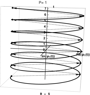
Figure 1: The helix for the function $\psi_{1}(t)$, with $P=1$ and $-5\leq t\leq 7$.

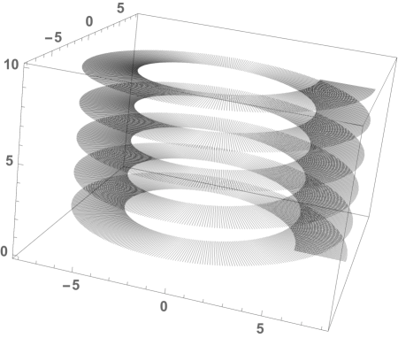
Figure 2: Double helix: 1-Lucas and 2-Lucas $(0\leq t\leq 10$).

4 Examples

In the next examples we apply the complex expressions $g(t),h(t),\psi_{1}(t),\psi_{2}(t)$ and $\psi_{3}(t)$, respectively defined in (6), (14) and (28), for several values of the integer parameter $P\geq 1$.

Given integers $t_{min}<t_{max}$ we considerer the interval $[t_{min},t_{max}]$ for domain of the real independent variable $t$. The corresponding curves has been obtained by computing the real and imaginary parts of the maps $g,h,\psi_{1},\psi_{2}$ and $\psi_{3}$. The computer algebra system Mathematica [15] has been used to display the corresponding helical curves, by means of the built-in commands $\verb+Re[ ]+$, $\verb+Im[ ]+$ and $\verb+ParametricPlot3D[ ]+$.

The resulting helices are presented in order to confirm and illustrate Propositions 2.1 and 3.1. We also introduce some double helices resulting from a combination of Lucas/Fibonacci helices. Other double and triple helices will be discussed in a forthcoming work.

Example 4.1.

For $P=1$ we have $D=P^{2}+4=5$. Lucas sequence is

$$2,1,3,4,7,11,18,29,\ldots,$$

and the Fibonacci sequence is

$$0,1,1,2,3,5,8,13,21,\ldots\ .$$

The respective maps $g$ and $h$ are

$$\begin{array}[]{l}g(t)=\displaystyle\frac{1}{2^{t}}\left((1+\sqrt{5})^{t}+(1-\sqrt{5})^{t}\right)\\ \\ h(t)=\displaystyle\frac{1}{\sqrt{5}\,2^{t}}\left((1+\sqrt{5})^{t}-(1-\sqrt{5})^{t}\right),\qquad t\in\mathbb{R}\ .\end{array}$$ (35)

The functions $\psi_{1}$, $\psi_{2}$ and $\psi_{3}$ have the following expressions:

$$\begin{array}[]{ll}\psi_{1}(t)=g^{2}(t)-g(t-1)\,g(t-2)=5\,(-1)^{t}&\mbox{ (Lucas)}\\ \psi_{2}(t)=h(t-1)\,h(t+1)-h^{2}(t)=(-1)^{t}&\mbox{ (Fibonacci)}\\ \psi_{3}(t)=g^{2}(t)-D\,h^{2}(t)=4\,(-1)^{t},\quad t\in\mathbb{R}&\mbox{ (Pell),}\\ \end{array}$$ (36)

which show that these maps are representable as helices with ratios 5, 1 and 4 respectively.

For $P=1$, the Lucas helix is displayed in Figure 1, where the respective lattice points are shown by means of bold black points. As theoretically expected it is clear that the displayed dashed arrows connecting two consecutive lattice points belong to the vertical plane defined by the $x$ and $z$ axes.

Example 4.2.

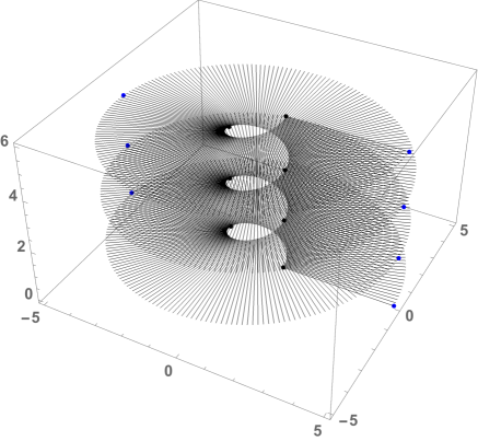
Figure 3: Double helix: 1-Lucas to 2-Fibonacci.

In Figure 2 we show a double helix. It results from connecting the point $\psi_{1}(t)$ with $P=1$ to the point $\psi_{1}(t)$ with $P=2$, for $t\in[0,10]$. The respective graph was obtained discretising the variable $t$ taking $t_{min}=0$ to $t_{max}=10$ and increments $dt=0.005$. The inner helix (with $P=1$) has ratio $R=p^{2}+4=5$, while the outer helix (with $P=2$) has ratio $2^{2}+4=8$, as expected.

Example 4.3.

Using analogous technique as in Example 4.2, the next double helix (Figure 3) connects a 1-Lucas helix to a 2-Fibonacci helix. Thus the resulting double helix has interior ratio $R=1$ (for 2-Fibonacci) and exterior ratio $R=5$ (for 1-Lucas). Figure 4 displays a lateral (right) view of the helix in Figure 3, confirming that its lattice points belong to the vertical plane $xz$.

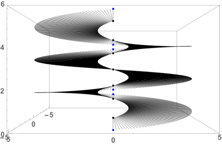
Figure 4: Double helix: 1-Lucas to 2-Fibonacci (right view).

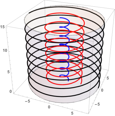
Figure 5: Helices of Lucas (black), Pell (red) and Fibonacci (blue), for $P=2$.

Example 4.4.

In Figure 5 we show a cylinder containing three helices, for $0\leq t\leq 15$ and $P=2$. The outer helix results from $\psi_{1}(t)=8\,(-1)^{t}$ (Lucas) and the inner one from $\psi_{2}(t)=(-1)^{t}$ (Fibonacci). As expect the middle helix corresponds to $\psi_{3}(t)=4\,(-1)^{t}$ (Pell). The ratios of these helices are in accordance to the values of $R$ in Table 1.

References

[1] J. Adam, Putting the in Biology: A review of the Mathematics of Life, Notices AMS 58 (2011), 1572-1578.
[2] A. Capanna, Architecture, form, expression. The helicoidal skycraper’s geometry.
AMS conference held at Towson University – Bridges 2012: Mathematics, Music, Architecture, Culture (2012), 349-356.
[3] H. Cohen, Number Theory, Volume I: Tools and Diophantine Equations, Springer, 2007.
[4] K. Devlin, Finding Fibonacci: The Quest to Rediscover The Forgotten Mathematical Genius Who Changed the World, Princeton University Press, 2017.
[5] M. Edson, O. Yayenie, A new generalization of Fibonacci sequence and extended Binet’s formula, Integers 9 (2009), 639-654.
[6] S. Falcón, A. Plaza, On the 3-dimensional -Fibonacci spirals, Chaos Solitons and Fractals (2008), 993-1003.
[7] V. E. Hoggatt, Jr., Fibonacci and Lucas Numbers, The Fibonacci Association, University of Santa Clara, 1969.
[8] D. Huylebrouck, P. Labasque, More true applications of the golden number, Nexus Network Journal 4, No.1 (2002), 45-58.
[9] H. W. Lenstra Jr., Solving the Pell equation, Notices AMS 49, Number 2 (2002), 182-192.
[10] T. Needham, Visual Complex Analysis, Clarendon Press, Oxford, 2004.
[11] A. Stakhov, B. Rozin, Theory of Binet formulas for Fibonacci and Lucas- numbers, Chaos Solitons and Fractals 27 (2006) 1162-1167.
[12] I. Stewart, The Mathematics of Life, Basic Books, New York, 2011.
[13] J. D. Watson, The Double Helix: A Personal Account of the Discovery of the Structure of DNA, Simon and Schuster, New York, 1968.