Note on Accuracy of the Post-Newtonian Approximation for Extreme-Mass Ratio Inspirals: Retrograde Orbits

Abstract

The post-Newtonian approximation is useful to discuss gravitational waveforms for binary inspirals. In this note, for retrograde circular orbits in the equatorial plane, we discuss the region of validity of the post-Newtonian approximation by using the gravitational energy flux derived numerically and analytically in the black hole perturbation approach. It is found that the edge of the allowable region behaves quite intricately, including prograde orbits even if we treat higher post-Newtonian orders.

1 Introduction

The post-Newtonian (PN) approximation (see, e.g., [1, 2] for a review) is widely used not only to derive gravitational waveforms for binary inspirals, but also to prepare initial parameters for numerical relativity (NR) simulations (see, e.g., [3, 4, 5] for quasicircular initial parameters of binary black hole (BBH) simulations).

In the PN approximation, we assume the slow-motion/weak-field. To treat the PN approximation, it is important to know where the above assumptions are appropriate. In the case of quasicircular binaries, the region of validity of the PN approximation is expressed, for example, by the orbital radius.

Using the PN energy flux for extreme mass ratio inspirals (EMRIs) in the black hole (BH) perturbation approach, the region of validity of the PN approximation has been discussed in [6, 7, 8] (see also [9]). Since we use the assumption of $\mu\ll M$ where the EMRIs are described by a point particle with mass $\mu$ orbiting around a BH with mass $M$, in this approach, it is possible to calculate the energy flux numerically and analytically up to very high PN orders. In our previous paper [10], we treated the numerical energy flux derived in [11, 12] and the PN flux in [13] (see also [14, 15, 16]) for prograde circular orbits in the Kerr spacetime, and analyzed the region of validity. Although there are some large region of validity for some PN order (see, e.g., the top panel of Figure 1 in [10] where the 3PN order ($N=6$) has a larger region of validity than that of the 3.5PN order ($N=7$)), we have found that higher PN orders give a larger region of validity as expected. In our previous paper and this note, we note that the region of validity is discussed for the gravitational energy flux, i.e. the time-averaged dissipative piece of the first-order gravitational self-force (GSF). We do not consider the conservative piece of the first-order GSF in this note.

Here, an important circular orbit in the equatorial plane is the innermost stable circular orbit (ISCO). The ISCO radius in Boyer-Lindquist coordinates is given as [17]

$$\frac{r_{\rm ISCO}}{M} = 3+Z_{2}\mp\sqrt{(3-Z_{1})(3+Z_{1}+2Z_{2})}\,,$$ (1)

where

$$Z_{1} = 1+(1-(a/M)^{2})^{1/3}[(1+a/M)^{1/3}+(1-a/M)^{1/3}]\,,$$ (2)

$$Z_{2} = \sqrt{3(a/M)^{2}+Z_{1}^{2}}\,,$$ (3)

and the upper and lower signs refer to the prograde (direct) and retrograde orbits (with the Kerr parameter $0\leq a\leq M$), respectively. Given the orbital radius $r$, the orbital velocity is calculated by

$$v=(M\Omega)^{1/3}\,;\quad M\Omega=\frac{M^{3/2}}{r^{3/2}+aM^{1/2}}\,.$$ (4)

In Table 1, the ISCO radius, frequency and velocity are summarized for various $a/M$.

Table 1: The ISCO radius ($r_{\rm ISCO}$), frequency ($\Omega_{\rm ISCO}$) and velocity ($v_{\rm ISCO}$) for various Kerr spin parameters ($a$).

$a/M$	$r_{\rm ISCO}/M$	$M\Omega_{\rm ISCO}$	$v_{\rm ISCO}$
1.0 (retrograde)	9.000000000	0.03571428571	0.3293168780
0.9 (retrograde)	8.717352279	0.03754018063	0.3348359801
0.5 (retrograde)	7.554584713	0.04702732522	0.3609525320
0.0	6.000000000	0.06804138173	0.4082482904
0.5 (prograde)	4.233002531	0.1085883589	0.4770835292
0.9 (prograde)	2.320883043	0.2254417086	0.6086179484
1.0 (prograde)	1.000000000	0.5000000000	0.7937005260

For the retrograde ISCOs in Table 1, we see larger ISCO radii, smaller ISCO frequencies and velocities than those for the prograde ISCOs. As a naive expectation, the region of validity of the PN approximation for the retrograde case will be smaller than that for the prograde case. Despite this spin dependence, we usually require a same frequency for various configuration to produce hybrid PN-NR waveforms [18, 19]. Also, we need to search gravitational waves (GWs) with various spin directions of binary systems since the plausible spin direction is not known. Interestingly, a recent GW event, GW170104 suggests that both spins aligned with the orbital angular momentum of the BBH system are disfavored [20].

In our previous paper [10], we only discussed several cases of prograde orbits and did not discuss retrograde orbits since we expected that the region of validity in the PN approximation for retrograde orbits would behave similar to that for prograde ones. Motivated by the observation of GW170104, however, we reanalyze the region of validity in the PN approximation both for prograde and retrograde orbits more carefully and find complicated behaviors in the region of validity which have not been noticed in our previous paper (see, e.g., Fig. 2). We would expect that additional results might be of interest to people working on numerical relativity simulations, and would like to summarize results in this note.

The note is organized as follows. In Section 2, we review the definition of the edge of allowable region (AR) briefly which was introduced in our previous paper [10]. In Section 3, we show the edge of the allowable region from the eccentricity estimation for retrograde circular orbits in the equatorial plane. Finally, we summarize and discuss the results presented in our previous paper and this note in Section 4. In this note, we use the geometric unit system, where $G=c=1$.

2 Edges of the allowable region

To discuss the region of validity of the PN approximation, we use the gravitational energy flux $F_{g}$ for a point particle orbiting in circular orbits around a BH. The basic equations in the BH perturbation approach are the Regge-Wheeler-Zerilli [21, 22] and Teukolsky [23] equations. The energy flux is computed in two ways: one is the numerical approach which gives the “exact” value in the numerical accuracy, and the other is the analytical approach where we employ the PN approximation.

In the analytical approach, the gravitational energy flux is written as

$$\frac{dE^{(N)}}{dt}=-F_{\rm Newt}F^{(N)}\,,$$ (5)

where $F_{\rm Newt}$ is the Newtonian flux,

$$F_{\rm Newt}=\frac{32}{5}\left(\frac{\mu}{M}\right)^{2}v^{10}\,,$$ (6)

and $F^{(N)}$ is the ($N/2$)PN result normalized by the Newtonian flux. $v$ is the circular orbital velocity. We denote the exact value obtained in the numerical approach as $F$.

In our previous paper [10], we followed the analyses presented in [7] (based on [24]) and obtained consistent results with [7, 8]. As an alternative method which is the simplest analysis and a practical method for the region of validity, we have considered an allowance $\delta$ for the difference between the numerical and analytical results as

$$|F-F^{(N)}|<\delta\,.$$ (7)

Here, when we discuss the quasicircular evolution, the deviation from the exact energy flux induces the “artificial” orbital eccentricity $e$, that shows the deviation from the “exact” quasicircular evolution. Assuming the eccentric orbit with a semimajor axis $r_{0}$,

$$r(t)\sim r_{0}\left[1-e\cos\left(\frac{vt}{r_{0}}\right)\right]\,.$$ (8)

where we have already known that the Newtonian orbit is sufficient to estimate the eccentricity [10], the orbital eccentricity is expressed as

$$e\equiv \left(\frac{dE}{dr}\right)^{-1}\frac{1}{v}\,F_{\rm Newt}\,|F-F^{(N)}|\,,$$ (9)

where $E$ is the orbital energy of the particle,

$$\frac{E}{\mu}= {\frac{{r}^{3/2}-2\,M\sqrt{r}+a\sqrt{M}}{{r}^{3/4}\left({r}^{3/2}-3\,M\sqrt{r}+2\,a\sqrt{M}\right)^{1/2}}}\,.$$ (10)

The relation between the orbital radius and velocity is given by (4).

In NR simulations of BBH [25, 26, 27], an iterative procedure to obtain low-eccentricity initial orbital parameters is used [28, 29, 30, 31, 32]. According to [32], we need a $t=O(1000M)$ numerical evolution (where $M$ denotes the total mass for comparable mass binaries) to reduce the eccentricity by about a factor of 10. For example, we find the eccentricity in the initial parameters for NR simulations of GW150914 [33, 34, 35, 36] is $\sim 0.0012$ (RIT) and $0.0008$ (SXS) [37] (see also BBH simulation catalogs [38, 39, 40, 41] and references therein). Since quasicircular initial parameters are an important input for NR simulations [42], we treat the edge of the allowable region by using the eccentricity to discuss the region of validity of the PN approximation.

3 Results

We set a restriction on $e$ from the error in the energy flux as

$$e\leq 1\times 10^{-5}\,,$$ (11)

where this reference value is adopted from the lowest eccentricity in NR simulations presented in [18]. Combining (9) with (11), the edge of the allowable region is presented in terms of the orbital velocity (top), $v^{(N)}$, and radius (bottom) for retrograde circular orbits in Kerr ($q=a/M=0,\,-0.1,\,-0.3,\,-0.5,\,-0.9$) cases in Figure 1. Here, the (normalized) numerical energy flux $F$ and the (normalized) PN flux $F^{(N)}$ in (9) are calculated by [11, 12] and [13], respectively.

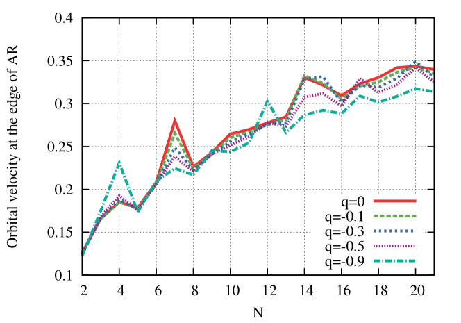
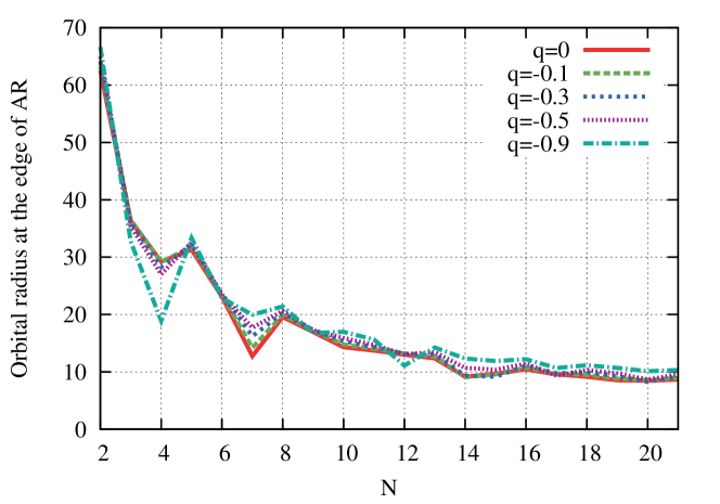
Figure 1: The edge of the allowable region from the eccentricity estimation in the case of $e\leq 1\times 10^{-5}$ in terms of the orbital velocity (top) and radius (bottom).

At 3.5PN order ($N=7$), we see a clear tendency for the allowable region to decrease when $q$ becomes more negative. Also, in large $N$, the allowable region for large negative $q$ values has a similar behavior to the ISCO given in (1) (see also Table 1 and Figure 2), but it is not so clear.

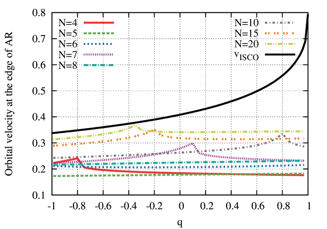
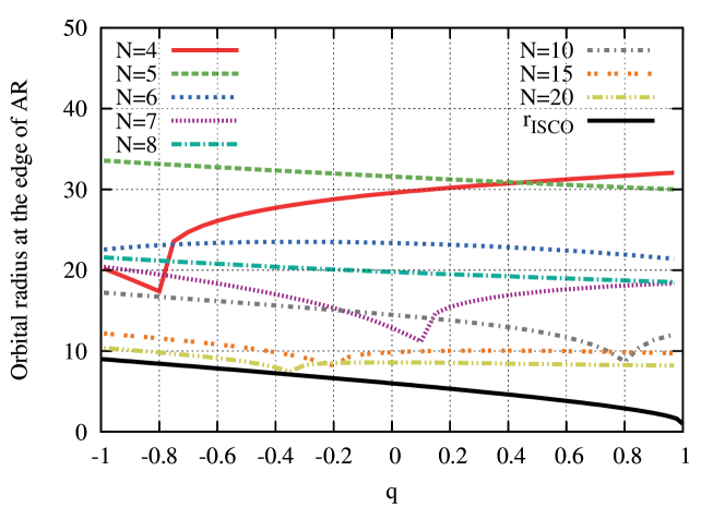
Figure 2: Edges of the allowable region for the orbital velocity $v_{\rm AR}$ (top) and radius $r_{\rm AR}$ (bottom) for all range of the non-dimensional Kerr parameter, $q=a/M$. Here, $q>0$ and $q<0$ are for prograde and retrograde orbits, respectively.

4 Summary and Discussions

In this note, we have used EMRIs for the analysis. For the current ground-based GW detectors, Advanced LIGO (aLIGO) [43], Advanced Virgo (AdV) [44], KAGRA [45, 46], comparable mass ratio binaries are the target. To extrapolate the result in this note to these binaries where individual objects have mass $m_{1}$ and $m_{2}$, and nondimensional spin $\chi_{1}$ and $\chi_{2}$, it may be possible to consider $M$, $\mu$ and $q=a/M$ as the total mass ($m_{1}+m_{2}$), the reduced mass ($m_{1}m_{2}/(m_{1}+m_{2})$) of the system, and an effective spin $\chi_{\rm eff}=(m_{1}\chi_{1}+m_{2}\chi_{2})/(m_{1}+m_{2})$ [47] (see also [48]), respectively.

Figure 2 shows the edges of the allowable region for the orbital velocity $v_{\rm AR}$ and radius $r_{\rm AR}$ from the eccentricity estimation ((9) with (11)) for all range of Kerr parameter. The ISCO values given in Table 1 are also shown. For example, it is found at 2.5PN and 4PN order ($N=5$ and $8$, respectively) that the orbital radius at the edge of the allowable region for large negative values of $q$ tends to be larger and has a similar $q$ dependence to the ISCO radius. This suggests that when we start numerical relativity simulations of binary systems with the 2.5PN and 4PN initial orbital parameters, we need to consider a larger initial orbital separation for large negative $q$ cases.

On the other hand, at 3.5PN order ($N=7$) the allowable region basically decreases for large $q$. This may be a possible reason why the initial parameters given by Ref. [42] for nearly maximally spinning BBH simulations [49] do not work well. It is noted in Figure 2 that discontinuous change with respect to $q$ arise from different sequences of solutions for the equality (9) with $e=1\times 10^{-5}$. The top panel of Figure 3 shows complicated behaviors of the right hand side of (9) for $N=7$ and various $q$ as a function of the orbital radius. From this figure, we can find that there are several solutions in the orbital radius for $q=0.20$ and $0.14$ when we set $e=1\times 10^{-5}$, while there is a single solution for $q=0.40$, $0.10$ and $0.05$. In the case that (9) has several solutions, we choose the largest solution in the orbital radius as the edge of the allowable region, which is larger than the one that gives the local maximum of the right hand side of (9). Then the solutions vary smoothly from $q=0.40$ to $q=0.14$. The discontinuous change of solutions in the orbital radius with respect to $q$ might appear between $q=0.14$ and $0.10$ when we set $e=1\times 10^{-5}$. This is because the local maximum of the right hand side of (9) for $q=0.10$ becomes smaller than $1\times 10^{-5}$ and the solution in the orbital radius for $q=0.10$ becomes smaller than the one that gives the local minimum of the right hand side of (9). The locations of discontinuities depend on the restriction on $e$. Contrarily, we see simple behaviors for $N=8$ in the bottom panel of Figure 3, and this gives the continuous variation in Figure 2. Even if we treat higher PN order, say, $N=20$, it is difficult to estimate a simple $q$-dependence of the edge of the allowable region. Therefore, the above conclusion derived from the 2.5PN and 4PN analyses is not held. We should note that any local peaks in Figures 1 and 2 do not indicate the best PN approximation in a given order as mentioned in [10]. We always welcome higher PN results in order to investigate whether the allowable region becomes larger.

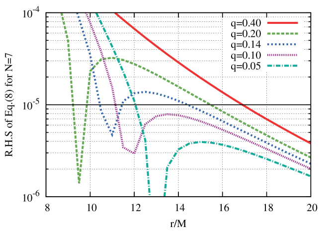
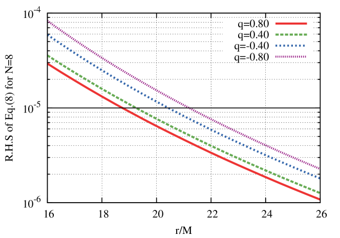
Figure 3: The right hand side of (9) as a function of the orbital radius for various non-dimensional Kerr parameters, $q=a/M$ in the case of $N=7$ (top) and $8$ (bottom).

Although the allowable region has been discussed for the gravitational energy flux, i.e., the first order dissipative self-force in our previous paper [10] and this note, the post-adiabatic effects of the self-force, i.e., the first order conservative and the second order dissipative self-forces should be studied. As for the Schwarzschild background, the radius of convergence of the PN series for the first order conservative self-force has been shown in [50] (see also [51]). For the Kerr case, It is possible to discuss the radius of convergence by using an analytic result presented in [52]. Furthermore, [53] is usable in the case of eccentric orbits around a Kerr BH. For future work, we will analyze the allowable region by using the above results to connect our analysis with the comparable mass ratio binaries.

References

References

- [1] L. Blanchet, Living Rev. Rel. 17, 2 (2014) [arXiv:1310.1528 [gr-qc]].
- [2] M. Sasaki and H. Tagoshi, Living Rev. Rel. 6, 6 (2003) [gr-qc/0306120].
- [3] J. G. Baker, M. Campanelli, C. O. Lousto and R. Takahashi, Phys. Rev. D 65, 124012 (2002) [astro-ph/0202469].
- [4] S. Husa, M. Hannam, J. A. Gonzalez, U. Sperhake and B. Bruegmann, Phys. Rev. D 77, 044037 (2008) [arXiv:0706.0904 [gr-qc]].
- [5] M. Campanelli, C. O. Lousto, H. Nakano and Y. Zlochower, Phys. Rev. D 79, 084010 (2009) [arXiv:0808.0713 [gr-qc]].
- [6] E. Poisson, Phys. Rev. D 52, 5719 (1995) [Addendum-ibid. D 55, 7980 (1997)] [gr-qc/9505030].
- [7] N. Yunes and E. Berti, Phys. Rev. D 77, 124006 (2008) [Erratum-ibid. D 83, 109901 (2011)] [arXiv:0803.1853 [gr-qc]].
- [8] Z. Zhang, N. Yunes and E. Berti, Phys. Rev. D 84, 024029 (2011) [arXiv:1103.6041 [gr-qc]].
- [9] Y. Mino, M. Sasaki, M. Shibata, H. Tagoshi and T. Tanaka, Prog. Theor. Phys. Suppl. 128, 1 (1997) [gr-qc/9712057].
- [10] N. Sago, R. Fujita and H. Nakano, Phys. Rev. D 93, 104023 (2016) [arXiv:1601.02174 [gr-qc]].
- [11] R. Fujita and H. Tagoshi, Prog. Theor. Phys. 112, 415 (2004) [gr-qc/0410018].
- [12] R. Fujita and H. Tagoshi, Prog. Theor. Phys. 113, 1165 (2005) [arXiv:0904.3818 [gr-qc]].
- [13] R. Fujita, PTEP 2015, 033E01 (2015) [arXiv:1412.5689 [gr-qc]].
- [14] R. Fujita, Prog. Theor. Phys. 127, 583 (2012) [arXiv:1104.5615 [gr-qc]].
- [15] R. Fujita, Prog. Theor. Phys. 128, 971 (2012) [arXiv:1211.5535 [gr-qc]].
- [16] N. Sago and R. Fujita, PTEP 2015, 073E03 (2015) [arXiv:1505.01600 [gr-qc]].
- [17] J. M. Bardeen, W. H. Press and S. A. Teukolsky, Astrophys. J. 178, 347 (1972).
- [18] P. Ajith et al., Class. Quant. Grav. 29, 124001 (2012) Addendum: [Class. Quant. Grav. 30, 199401 (2013)] [arXiv:1201.5319 [gr-qc]].
- [19] J. Aasi et al. [LIGO Scientific and VIRGO and NINJA-2 Collaborations], Class. Quant. Grav. 31, 115004 (2014) [arXiv:1401.0939 [gr-qc]].
- [20] B. P. Abbott et al. [LIGO Scientific and VIRGO Collaborations], Phys. Rev. Lett. 118, 221101 (2017) [arXiv:1706.01812 [gr-qc]].
- [21] T. Regge and J. A. Wheeler, Phys. Rev. 108, 1063 (1957).
- [22] F. J. Zerilli, Phys. Rev. D 2, 2141 (1970).
- [23] S. A. Teukolsky, Astrophys. J. 185, 635 (1973).
- [24] C. M. Bender and S. A. Orszag, Advanced Mathematical Methods for Scientists and Engineers 1, Asymptotic Methods and Perturbation Theory (Springer, New York, 1999).
- [25] F. Pretorius, Phys. Rev. Lett. 95, 121101 (2005) [gr-qc/0507014].
- [26] M. Campanelli, C. O. Lousto, P. Marronetti and Y. Zlochower, Phys. Rev. Lett. 96, 111101 (2006) [gr-qc/0511048].
- [27] J. G. Baker, J. Centrella, D. I. Choi, M. Koppitz and J. van Meter, Phys. Rev. Lett. 96, 111102 (2006) [gr-qc/0511103].
- [28] M. Boyle, D. A. Brown, L. E. Kidder, A. H. Mroue, H. P. Pfeiffer, M. A. Scheel, G. B. Cook and S. A. Teukolsky, Phys. Rev. D 76, 124038 (2007) [arXiv:0710.0158 [gr-qc]].
- [29] H. P. Pfeiffer, D. A. Brown, L. E. Kidder, L. Lindblom, G. Lovelace and M. A. Scheel, Class. Quant. Grav. 24, S59 (2007) [gr-qc/0702106].
- [30] A. Buonanno, L. E. Kidder, A. H. Mroue, H. P. Pfeiffer and A. Taracchini, Phys. Rev. D 83, 104034 (2011) [arXiv:1012.1549 [gr-qc]].
- [31] M. Purrer, S. Husa and M. Hannam, arXiv:1203.4258 [gr-qc].
- [32] L. T. Buchman, H. P. Pfeiffer, M. A. Scheel and B. Szilagyi, Phys. Rev. D 86, 084033 (2012) [arXiv:1206.3015 [gr-qc]].
- [33] B. P. Abbott et al. [LIGO Scientific and Virgo Collaborations], Phys. Rev. Lett. 116, 061102 (2016) [arXiv:1602.03837 [gr-qc]].
- [34] B. P. Abbott et al. [LIGO Scientific and Virgo Collaborations], Phys. Rev. D 93, 122003 (2016) [arXiv:1602.03839 [gr-qc]].
- [35] B. P. Abbott et al. [LIGO Scientific and Virgo Collaborations], Phys. Rev. Lett. 116, 241102 (2016) [arXiv:1602.03840 [gr-qc]].
- [36] B. P. Abbott et al. [LIGO Scientific and Virgo Collaborations], Phys. Rev. D 93, 122004 (2016) Addendum: [Phys. Rev. D 94, 069903 (2016)] [arXiv:1602.03843 [gr-qc]].
- [37] G. Lovelace et al., Class. Quant. Grav. 33, 244002 (2016) [arXiv:1607.05377 [gr-qc]].
- [38] A. H. Mroue et al., Phys. Rev. Lett. 111, 241104 (2013) [arXiv:1304.6077 [gr-qc]].
- [39] K. Jani, J. Healy, J. A. Clark, L. London, P. Laguna and D. Shoemaker, Class. Quant. Grav. 33, 204001 (2016) [arXiv:1605.03204 [gr-qc]].
- [40] B. P. Abbott et al. [LIGO Scientific and Virgo Collaborations], Phys. Rev. D 94, 064035 (2016) [arXiv:1606.01262 [gr-qc]].
- [41] J. Healy, C. O. Lousto, Y. Zlochower and M. Campanelli, arXiv:1703.03423 [gr-qc].
- [42] J. Healy, C. O. Lousto, H. Nakano and Y. Zlochower, arXiv:1702.00872 [gr-qc].
- [43] J. Aasi et al. [LIGO Scientific Collaboration], Class. Quant. Grav. 32, 074001 (2015) [arXiv:1411.4547 [gr-qc]].
- [44] F. Acernese et al. [VIRGO Collaboration], Class. Quant. Grav. 32, 024001 (2015) [arXiv:1408.3978 [gr-qc]].
- [45] K. Somiya [KAGRA Collaboration], Class. Quant. Grav. 29, 124007 (2012) [arXiv:1111.7185 [gr-qc]].
- [46] Y. Aso et al. [KAGRA Collaboration], Phys. Rev. D 88, 043007 (2013) [arXiv:1306.6747 [gr-qc]].
- [47] P. Ajith et al., Phys. Rev. Lett. 106, 241101 (2011) [arXiv:0909.2867 [gr-qc]].
- [48] T. Damour, Phys. Rev. D 64, 124013 (2001) [gr-qc/0103018].
- [49] Y. Zlochower, J. Healy, C. O. Lousto and I. Ruchlin, arXiv:1706.01980 [gr-qc].
- [50] N. K. Johnson-McDaniel, A. G. Shah and B. F. Whiting, Phys. Rev. D 92, 044007 (2015) [arXiv:1503.02638 [gr-qc]].
- [51] C. Kavanagh, A. C. Ottewill and B. Wardell, Phys. Rev. D 92, 084025 (2015) [arXiv:1503.02334 [gr-qc]].
- [52] C. Kavanagh, A. C. Ottewill and B. Wardell, Phys. Rev. D 93, 124038 (2016) [arXiv:1601.03394 [gr-qc]].
- [53] D. Bini, T. Damour and A. Geralico, Phys. Rev. D 93, 124058 (2016) [arXiv:1602.08282 [gr-qc]].