The Role of Mastery Learning in an Intelligent Tutoring System: Principal Stratification on a Latent Variable

Abstract

Students in Algebra I classrooms typically learn at different rates and struggle at different points in the curriculum—a common challenge for math teachers. Cognitive Tutor Algebra I (CTA1), educational computer program, addresses such student heterogeneity via what they term “mastery learning,” where students progress from one section of the curriculum to the next by demonstrating appropriate “mastery” at each stage. However, when students are unable to master a section’s skills even after trying many problems, they are automatically promoted to the next section anyway. Does promotion without mastery impair the program’s effectiveness?

At least in certain domains, CTA1 was recently shown to improve student learning on average in a randomized effectiveness study. This paper uses student log data from that study in a continuous principal stratification model to estimate the relationship between students’ potential mastery and the CTA1 treatment effect. In contrast to extant principal stratification applications, a student’s propensity to master worked sections here is never directly observed. Consequently we embed an item-response model, which measures students’ potential mastery, within the larger principal stratification model. We find that the tutor may, in fact, be more effective for students who are more frequently promoted (despite unsuccessfully completing sections of the material). However, since these students are distinctive in their educational strength (as well as in other respects), it remains unclear whether this enhanced effectiveness can be directly attributed to aspects of the mastery learning program.

, and

1 Introduction

Teaching a class full of students who vary widely in ability is one of the toughest challenges teachers face. Intelligent tutoring systems may help. These are pieces of software that are designed to act as tutors, teaching material to individual students working on computers (Anderson et al., 1985). Typically, they measure students’ relevant skill sets and present them with personalized problems or exercises. The students’ performance on these exercises determines what they work on next, based on updated measurements of their skill profiles. This process is referred to as “mastery learning”; students learn by mastering skills, and only then moving on to new material (Bloom, 1968; Kulik et al., 1990). The hope is that by personalizing learning, intelligent tutors can help teachers handle academic diversity.

Pane et al. (2014) reported the results of large-scale effectiveness study of the Cognitive Tutor Algebra I (CTA1), a curriculum whose centerpiece is the Cognitive Tutor software. In the second year of implementation, the study found a moderate positive effect of CTA1 on high school post-test scores.

While CTA1 is designed around mastery learning, it does not always work that way in practice (Israni et al., 2018). For instance, the CTA1 system sets a maximum number of problems students may work in each section. Occasionally, some students will be unable to master a set of skills before reaching the maximum number of problems. In those cases, rather than allow the student’s “wheel-spinning” (c.f. Beck and Gong, 2013) to continue indefinitely, CTA1 “promotes” them to the next section. Does the CTA1 treatment effect suffer as a result? Do students who are more frequently promoted tend to experience smaller treatment effects?

Student mastery is only defined subsequent to treatment assignment—students in the control condition do not use the software and therefore have no mastery data. Traditional causal inference models, such as analysis of covariance and subgroup analysis, can estimate the heterogeneity of treatment effects as a function of pre-treatment covariates but cannot accommodate variables that may themselves be a function of the treatment. On the other hand, principal stratification (Frangakis and Rubin, 2002; Page, 2012; Feller et al., 2016b; Sales et al., 2016) is designed for precisely such a task. A principal stratification analysis could estimate the variance of treatment effects as a function of potential mastery: how often a student would master worked sections, if assigned to treatment. This variable is defined prior to treatment assignment for all students in the study, but only observed for treatment students.

Implicitly, this assumes that potential mastery is measured without error in the treatment group, an untenable assumption in our case. There are no error-free measurements of students’ propensity to master sections. Further complicating matters, both the number of worked sections and which sections students worked varied widely between students in the treatment group. The typical principal stratification approach, assuming intermediate variables measured without error, may yield misleading or uninterpretable results when applied to mastery learning in CTA1.

This paper addresses the problem using a novel approach, combining principal stratification modeling with item response theory (IRT; e.g. Embretson and Reise, 2013) and latent variable analysis. Using an IRT model to measure student mastery potential as a latent variable brings a number of advantages over more traditional approaches. In particular, model-based measurement can account for variation in both the number of sections students work, and which sections students work, in addition to measurement error and missing data in general. Defining principal strata based on latent variables may dramatically broaden the set of questions principal stratification may answer.

The structure of the paper is as follows. The following section describes the CTA1 program, the CTA1 effectiveness trial, and the dataset. Next, Section 3 reviews and illustrates continuous Bayesian principal stratification. Section 4 introduces an IRT model for mastery and shows that it solves a number of problems with conventional approaches. Section 5 discusses incorporating a latent variable into Bayesian principal stratification. Section 6 specifies a model for the CTA1 dataset and discusses its identification; its results are in Section 7 and model checks are in Section 8. Section 9 concludes with critical discussions of the methodological advances and the meaning of the model results for intelligent tutoring systems.

2 Background

2.1 The Cognitive Tutor

CTA1 is one of a series of complete mathematics curricula developed by Carnegie Learning, Inc., which include both textbook materials and an automated computer-based Cognitive Tutor (Anderson et al., 1995).The CTA1 software divides the algebra course into units and sections within units. These are organized into a standard progression based on mathematics standards; however, schools have the option to customize these to meet local standards or other constraints. Many schools in the study exercised this option, meaning that although the basic set of sections and units is the same across the study, the sequence students encounter them is not.

The essential material of each section is represented as a set of fine-grained knowledge components, or skills, and the software is continually evaluating student mastery of these skills through the use of a detailed computational model of student thinking in algebra. Students solve problems and the model evaluates each student action—whether it is a correct or incorrect action on a path toward solving the problem, or a request for the software to provide a hint—and updates its assessment of the mastery of each skill. When students are judged to have mastered each skill in a section, they are automatically moved to the next section. In an exception to this general approach, when students work the maximum number of problems in a section without mastering its skills, they are deemed to be “wheel spinning.” The software promotes wheel-spinning students to the next section, despite their non-mastery. The system also enables teachers to override the mastery-based advancement to move students into a different section.

2.2 The CTA1 Effectiveness Trial

In 2007, the RAND Corporation received a grant from the U.S. Department of Education to evaluate the effectiveness of CTA1, when implemented without any extraordinary support, in a diverse set of schools. The project conducted two parallel experiments, one in 74 middle schools and one in 73 high schools, from 52 school districts in seven states. Participating schools include urban, suburban, and rural public schools, and some Catholic Diocese parochial schools, in Texas, Connecticut, New Jersey, Alabama, Michigan, and Louisiana. Each school participated for two years. Schools in each state participated in both the middle school and high school arms of the study except Alabama (middle school only). Nearly 18,700 high school students participated in the study.

The study used a blocked cluster randomized design to assign schools to study condition. Schools within each state were matched into pairs or triples, and randomized within blocks in the spring prior to their first year of implementation. Schools randomized to the treatment group implemented the CTA1 curriculum and those assigned to the control group continued to use their existing algebra I curriculum. Nearly all sites used materials published by Prentice Hall, Glencoe, or McDougal Littell. Assignments to treatment or control groups continued for two academic years in each school.

The study administered an algebra readiness pretest and an algebra proficiency post-test from the CTB/McGraw-Hill Acuity series. The exams were scored using a three-parameter IRT model. In the high school study, models estimated 95% confidence intervals for the treatment effect of -0.10$\pm$0.2 standard deviations in first year and 0.22$\pm$0.2 in the second year. In the middle school study, models estimated treatment effect confidence intervals of -0.03 $\pm$0.2 the first year and 0.19$\pm$0.3 the second year.

2.3 Data for Principal Stratification

Since our goal was to better understand the CTA1 treatment effect, we focused our analysis on data from high school students in the second year of the CTA1 trial, for whom the treatment effect was most evident.

We merged data from two sources: covariate, treatment and outcome data gathered by RAND, and computerized log data gathered by Carnegie Learning. Table 1 describes the covariates we used, including missingness information, control and treatment means, and standardized differences (c.f. Kalton, 1968). We singly-imputed missing values with the Random Forest routine implemented by the missForest package in R (Stekhoven and Buehlmann, 2012; R Core Team, 2016), which estimated the “out of box” imputation errors also shown in Table 1 as part of the random forest regression.

	% Miss.	Imp. Err.	Levels	Ctl.	Trt.	Std. Diff.
Ethnicity	8%	0.23	White/Asian	47%	52%	0.16
			Black/Multi	32%	26%	-0.14
			Hispanic/Nat.Am.	21%	22%	-0.03
Sex	4%	0.35	Female	51%	49%	-0.04
			Male	49%	51%	0.04
Sp. Ed.	1%	0.11	Typical	87%	86%	-0.00
			Spec. Ed	8%	8%	-0.02
			Gifted	5%	6%	0.03
Pretest	18%	0.20		-0.33	-0.36	-0.05
			Overall Covariate Balance: p=0.22

Table 1: Missingness information and balance for the covariates included in this study, from the CTA1 Effectiveness experiment, high school, year two. Imputation error is percent falsely classified for categorical variables (Race/Ethnicity, Sex, and Special Education) and standardized root mean squared error for Pretest, which is continuous. Analysis done in R via RItools (Bowers et al., 2017).

Over the course of the effectiveness study, Carnegie Learning gathered log data from student users, including mastery or promotion for each section each student encountered. Ninety-five control students (3% of the control group) appeared in the mastery dataset, presumably because they transferred from schools assigned to the control condition to treatment schools. We assumed that treatment assignment did not impact students’ decisions to transfer schools, and analyzed these students as control students, excluding their mastery data from the analysis.

Log data were missing for some students, either because the log files were not retrievable, or because of an imperfect ability to link log data to other student records. Treatment schools with mastery data missing for 90% or more students were omitted from the analysis, along with their entire randomization block. Of the remaining 2390 students, 84% had mastery data; treatment of missing mastery data for treatment students is discussed below, in Section 5.

Mastery data for sections that were not part of the standard CTA1 Algebra I curriculum, sections worked by fewer than 100 students, and sections that were mastered in every case were omitted from the dataset. The structure of the statistical model, described in section 6, justifies omitting these sections; a sensitivity check including all Algebra I sections and every school in the dataset yielded similar results.

Finally, because students’ characteristics and behavior were of primary interest, we included only data from worked sections that ended in either mastery or promotion, omitting cases in which the teacher moved the student to a new section prior to completion.

All told, the main analysis included $n=$5308 students, 2390 of whom were assigned to the CTA1 condition and 2918 of whom were assigned to control. The students were nested within 116 teachers, in 43 schools across five states. The analysis includes mastery information from 86,677 worked sections, 82% of which were mastered.

3 Principal Stratification for the CTA1 Experiment

In the CTA1 experiment, let $Z_{i}\in\{0,1\}$ represent student $i$’s treatment assignment, $i=1,\dots,N$. Let $Y_{i}$ denote $i$’s post-test score, so the central aim of the experiment was to estimate the average effect of $Z$ on $Y$. Following Neyman (1923) and Rubin (1978) let $Y_{Ti}$ and $Y_{Ci}$ denote $i$’s “potential” post-test scores were $Z_{i}=1$ or $Z_{i}=0$, respectively—that is, were $i$ assigned to treatment or control. This notation implicitly assumes the “Stable Unit Treatment Value Assumption,” or SUTVA (Rubin, 1980): that there was only one version of the treatment, and (since treatment was assigned at the school level) that one school’s treatment assignment did not affect outcomes in other schools. Then the observed test score $Y_{i}=Z_{i}Y_{Ti}+(1-Z_{i})Y_{Ci}$. For each subject $i$ let $\bm{x}_{i}$ denote a vector of pre-treatment covariates.

Let $\tau_{i}=Y_{Ti}-Y_{Ci}$, $i$’s treatment effect. Without strong untestable assumptions, $\tau_{i}$ is unidentified, since for each $i$, either $Y_{Ti}$ or $Y_{Ci}$ is unobserved. However, average treatment effects $\mathbb{E}[\tau]=\mathbb{E}[Y_{T}]-\mathbb{E}[Y_{C}]$ are identified. Similarly, randomization and SUTVA allow analysts to estimate treatment effects conditional on a variable $x$, say $\mathbb{E}[\tau|x]$, so long as $x$ was not itself affected by treatment assignment—for instance, gender or pretest scores.

The same cannot be said for so-called “intermediate variables” that are themselves affected by treatment assignment. Take $\bar{m}$, the proportion of a student’s worked sections that he or she mastered: $\bar{m}_{i}=\sum_{s}m_{is}/n^{sec}_{i}$, where $m_{is}=1$ if student $i$ mastered section $s$ and is zero otherwise. $n^{sec}_{i}$ is the number of sections student $i$ worked, $n^{sec}_{i}=\sum_{s}w_{si}$, where $w_{si}$ is an indicator which equals one if student $i$ works section $s$ until either mastery or promotion and zero otherwise. Since the CT software was unavailable for control students, $\bar{m}$ is only defined for treatment students. On the other hand, (following Frangakis and Rubin 2002) let $\bar{m}_{Ti}$ represent the proportion of sections that $i$ would master if assigned to the treatment condition—a potential value. Unlike $\bar{m}$, $\bar{m}_{T}$ is defined for all subjects prior to randomization, but only observed for members of the treatment group. For a control student $i$ with $Z_{i}=0$, $\bar{m}_{Ti}$ is a counterfactual, representing what would have happened had $i$ been assigned to treatment, i.e. had $Z_{i}=1$, counterfactually. Randomization guarantees that $\bar{m}_{T}$ is balanced—independent of treatment assignment (conditional on school and randomization block). Students who would master more sections, if given the opportunity, were no more or less likely to be assigned to treatment than those who would master fewer.

That being the case we may define a “principal effect” (c.f. Frangakis and Rubin, 2002, p. 23) as the super-population average treatment effect, conditional on $\bar{m}_{T}$:

$$\tau(m)\equiv\mathbb{E}[Y_{T}-Y_{C}|\bar{m}_{T}=m].$$ (3.1)

Since $\bar{m}_{T}$ is a continuous variable, Gilbert and Hudgens (2008) refer to $\tau(\cdot)$ as a “causal effect predictiveness curve” but we will follow Jin and Rubin (2008) and refer to $\tau(\cdot)$ as a principal effect, as in the more typical case of a categorical intermediate variable. (Typical principal stratification also requires conditioning on $\bar{m}_{C}$—the proportion of sections students would master if assigned to control—but this quantity is is undefined and irrelevant in our case, and may be dropped from the analysis.)

Potential mastery $\bar{m}_{T}$ is observed for treated students (for whom $\bar{m}_{T}=\bar{m}$), but unobserved for control students. That said, randomization ensures that the distribution of $\bar{m}_{T}$ conditional on pre-treatment covariates $\bm{x}$ is is the same in both treatment groups: $\bar{m}_{T}|\bm{x},Z=1=_{d}\bar{m}_{T}|\bm{x},Z=0$ (see Feller et al., 2016b, Lemmas 1 & 2). These facts allow for partial identification of principal effects.

Principal effects may be estimated via randomization inference (Nolen and Hudgens, 2011) or non-parametrically bounded (Miratrix et al., 2017). Most commonly, they are estimated with a Bayesian model (e.g. Li et al., 2015; Mattei et al., 2013). Jin and Rubin (2008) and Schwartz et al. (2011) give a full treatment of Bayesian principal stratification with a continuous intermediate variable such as $\bar{m}$, which we summarize here. Let $\bm{Z}$, $\bm{Y_{T}}$, $\bm{Y_{C}}$ and $\bm{\bar{m}_{T}}$ denote vectors of students’ treatment assignments, potential outcomes, and potential mastery proportions, and let $\bm{X}$ denote the covariate matrix formed by stacking row-vectors $\bm{x}^{T}$. Then randomization implies that $\bm{Z}$ is independent of $\bm{\bar{m}_{T}}$, $\bm{Y_{C}}$ and $\bm{Y_{T}}$, and hence is ignorable. Then, under exchangeability, for a vector of parameters $\bm{\theta}$ with prior density $f(\bm{\theta})$, we may write the joint distribution of $\bm{Y_{C}}$, $\bm{Y_{T}}$, and $\bm{\bar{m}_{T}}$ as:

$$f(\bm{Y_{C}},\bm{Y_{T}},\bm{\bar{m}_{T}}|\bm{X})\\ =\int\displaystyle\prod_{i}f(Y_{Ci},Y_{Ti}|\bar{m}_{Ti},\bm{x}_{i},\bm{\theta})f(\bar{m}_{Ti}|\bm{x}_{i},\bm{\theta})f(\bm{\theta})d\bm{\theta}.$$ (3.2)

This formulation allows for posterior inference via Markov Chain Monte Carlo techniques, such as data augmentation and Gibbs samplers (Gelman et al., 2014).

The model $f(\bar{m}_{Ti}|\bm{x}_{i},\bm{\theta})$ relates $\bar{m}_{T}$ to covariates. Though $\bar{m}_{Ti}$ is only observed for treated subjects, randomization ensures that the same model holds for both treatment groups, and hence is identified. The model $f(Y_{Ci},Y_{Ti}|\bar{m}_{Ti},\bm{x}_{i}\bm{\theta})$, relates potential outcomes to $\bar{m}_{T}$ and covariates. The model for treatment potential outcomes $f(Y_{Ti}|\bar{m}_{Ti},\bm{x}_{i},\bm{\theta})$, is entirely a function of observed variables, and is non-parametrically identified. In contrast, the model for control potential outcomes $f(Y_{Ci}|\bar{m}_{Ti},\bm{x}_{i},\bm{\theta})$ depends on unobserved $\bar{m}_{Ti}$; therefore, our analysis must rely on an assumed model. In practice, we we will assume that the model for $Y_{Ci}$ is drawn from the same family as $Y_{Ti}$, albeit with different parameters; see Richardson et al. 2011 for an in-depth treatment of analogous models. Of course, the fit of the $Y_{Ci}$ model may be compared to observed values $Y_{Ci}$ and $\bm{x}_{i}$.

With these models in place, posterior inference for parameters $\bm{\theta}$ proceeds by separating the two models into treatment and control observations:

$$f(\bm{\theta}|\bm{Y},\bm{Z},\bm{X},\bm{M}) \propto$$

$$f(\bm{\theta}) \displaystyle\prod_{i:Z_{i}=1}f(Y_{Ti},\bar{m}_{Ti}|\bm{x}_{i},\bm{\theta})$$

$$\times \displaystyle\prod_{i:Z_{i}=0}\int f(Y_{Ci}|\bm{x}_{i},\bm{\theta},\bar{m}_{Ti})f(\bar{m}_{Ti}|\bm{x}_{i},\bm{\theta})d\bar{m}_{Ti}.$$ (3.3)

Though $\bar{m}$ is unobserved for members of the control group, its conditional distribution may be estimated, and the marginal distribution of $Y_{C}$ may be recovered via integration.

Fitting principal stratification models is fraught with challenges; even when the model is well specified, multimodality and other pathologies of the likelihood function can bias standard estimation procedures (Griffin et al., 2008; Feller et al., 2016a). These results make clear that any model-based principal stratification analysis must include rigorous model checking and verification.

Figure 1 displays results from a principal stratification model, with $Y_{T}$ and $Y_{C}$ and $\bar{m}_{T}$ modeled as linear in covariates $\bm{x}$ with normally distributed errors clustered at the teacher and school levels, and with treatment effects linear in $\bar{m}_{T}$. Details are available in an online supplement (Sales and Pane, 2018). The x-axis of Figure 1 plots $\bar{m}_{T}$: for treated subjects, colored blue, the observed value, and for control subjects, colored red, the 1000th MCMC draw. The y-axis plots the observed posttest score $Y$. The figure also shows the 1000th MCMC draws of regression lines from the regressions of $Y_{T}$ and $Y_{C}$ on $\bar{m}_{T}$. Though $\bar{m}_{T}$ appears positively correlated with achievement in both treatment groups, the association is weaker in the treatment group than in the control group. This implies that students who would master a greater proportion of worked sections, if assigned to treatment, tend to experience lower treatment effects—CTA1 works best for students who tend to master fewer of the sections they work. The full posterior distributions of the regression lines, estimated via 4000 MCMC draws, are quite wide: a 95% credible interval for the difference between the lines’ slopes was $[-0.3,0.2]$ pooled posttest standard deviations per one interquartile range (IQR) of $\bar{m}_{T}$.

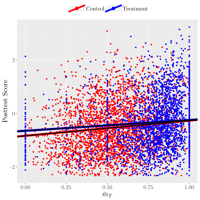
Figure 1: A posterior draw from a principal stratification model stratifying on $\bar{m}_{T}$: observed posttest scores (in pooled standard deviation units) as a function of $\bar{m}_{T}$, along with regression lines. $\bar{m}_{T}$ is observed for treated students group and imputed for control students.

4 Modeling Mastery

4.1 Problems with $\bar{m}$

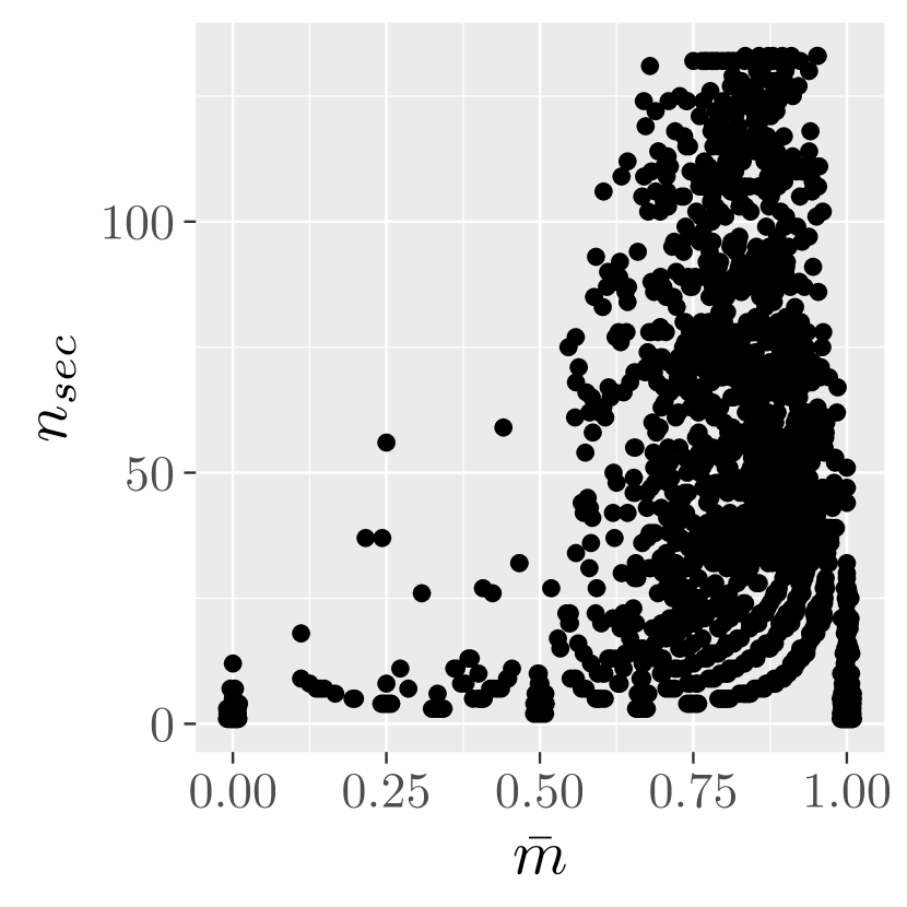
(a)

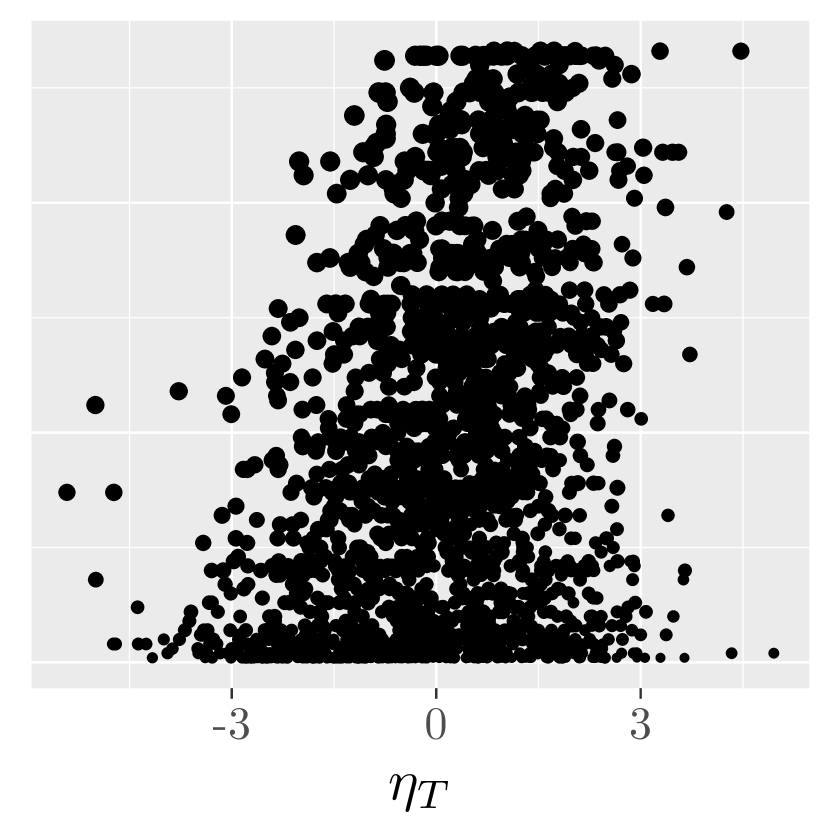
(b)

Figure 2: (a) Observed $\bar{m}$ as a function of $n^{sec}_{i}$. Overplotted points are jittered. (b) The 1,000th draw of $\eta_{Ti}$ for members of the treatment group as a function $n^{sec}$. $\eta_{Ti}$ is estimated from the model described by (4.1)–(6.3).

The principal stratification model based on $\bar{m}_{T}$, appears to be misspecified; Figure 1 shows clear differences between the distribution of $\bar{m}_{T}$ in the treatment group, observed as $\bar{m}$, and the distribution of imputed values for $\bar{m}_{T}$ in the control group. However, we shall see that even a well-specified model for $\bar{m}_{T}$ would yield misleading results.

Figure 2(a) shows $\bar{m}$ as a function of $n^{sec}$, the number of sections each student worked. As one might expect, there is a strong correspondence: extreme low values of $\bar{m}$ correspond almost exclusively to low values of $n^{sec}$. This mechanism appears to drive the leftward skew of the $\bar{m}$ distribution, and complicates any interpretation of an estimated function $\tau(m)$. In particular, it is hard to disentangle the respective roles $\bar{m}$ and $n^{sec}$ play in predicting treatment effects.

Students in the study vary not just in how many sections they attempt, but also in which sections they work. Figure 3(a) plots each treated student’s $\bar{m}$ as a function of the average estimated difficulty of the sections he or she worked (difficulty estimates are taken from the model we describe in the next section). A substantial amount of between-student variation in average section difficulty is apparent in Figure 3(a)—the difficulty estimates are fixed effects from a logistic regression, so near the center of their distribution a unit difference in section difficulty corresponds to a difference of roughly 25% in the probability of mastering a section (Gelman and Hill, 2006, p. 82). Unsurprisingly, students who work harder sections tend to master a smaller proportion; the Spearman correlation between $\bar{m}_{T}$ and average section difficulty is -0.30. Therefore, $\bar{m}$ is only partially a measure of students’ ability to master worked sections—it also measures which sections they worked.

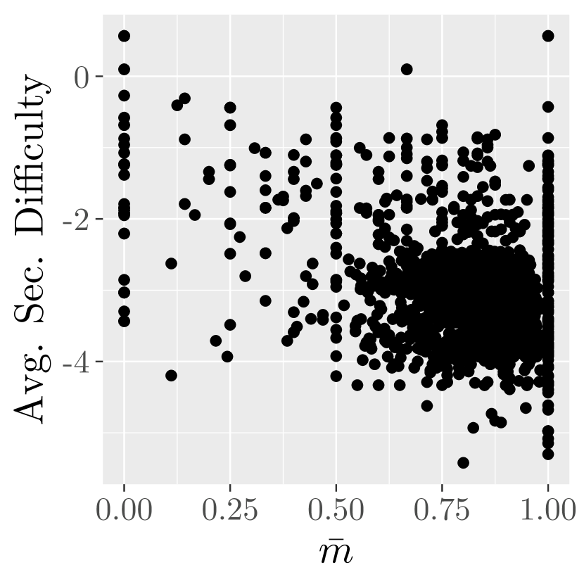
(a)

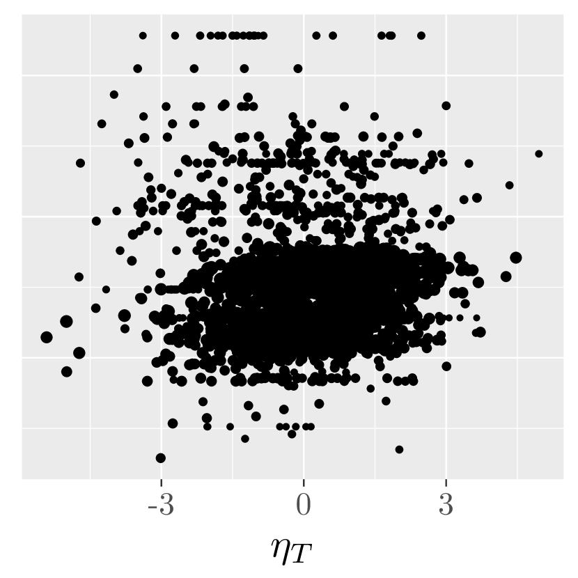
(b)

Figure 3: (a) Observed $\bar{m}$ for a student versus the average estimated difficulty of the sections he or she worked. Section difficulty was measured with the Rasch model (4.1)–(6.1). The within-student averages used estimates from the 1000th posterior draw. (b) The 1000th draw of $\eta_{T}$ versus average section difficulty.

4.2 IRT Mastery Models

A better measurement of student mastery must account for variation in the number of sections students worked, and their average difficulty. This is closely related to one of the initial motivations for IRT: comparing students’ scores across different tests of the same material (van der Linden and Hambleton, 2013). In applying IRT terminology to CTA1 mastery data, the “items” are sections that students work, and “responses” are binary indicators of mastery. This statistical structure is analogous to educational and psychological tests, the usual fodder for IRT models. On the other hand, the substantive difference between mastery on sections and responses to test questions requires careful attention.

Under the Rasch model (e.g. Rasch, 1993)—perhaps the simplest common IRT model—the probability that student $i$ masters worked section $s$ is:

$$Pr(m_{is}=1|w_{is}=1)=logit^{-1}(\eta_{Ti}-\delta_{s})$$ (4.1)

where $logit^{-1}(x)=\{1+exp(-x)\}^{-1}$ is the inverse logit function. The fixed “difficulty” parameter for section $s$, $\alpha_{s}$, in this case reflects the difficulty of achieving mastery on section $s$. The latent student “ability” $\eta_{Ti}$, modeled as a random intercept, represents student $i$’s propensity to master worked sections, since $Pr(m_{is}|w_{is};\eta_{Ti},\delta_{s})$ increases with increasing $\eta_{Ti}$.

Unlike in psychological testing, $\eta_{T}$ is not a measure of student ability, knowledge, or achievement—though it may correlate with these. The Cognitive Tutor’s principal aim is to help students master algebra skills, so $\eta_{Ti}$ may be thought of as a measure of whether CTA1 works as intended for student $i$. That is, mastery is CTA1’s own criterion of success. By definition, students who learn best from CTA1 are those who are more likely to master the sections they work.

Model (4.1) encodes a number of substantive assumptions about how and when sections are mastered. For instance, as suggested by an anonymous reviewer, it assumes that the probability a student masters a section does not depend on which other sections the student had previously worked. Fortunately, students mostly adhered to the standard section order imposed by Carnegie Learning, and almost always worked the sections in an order that respected pre-requisite structure (Israni et al., 2018). Along similar lines, it also assumes that a student’s propensity to master a worked section remains constant over the course of the study. This assumption would be violated if, for instance, students learned over time how to better interact with the software, and were thus able to master sections more reliably. This, in turn, would induce a correlation between $\eta_{Ti}$ and $n^{sec}_{i}$, so that the amount of student usage, and not just mastery, impacts $\eta_{T}$. Indeed, such a (rather slight) correlation appears to exist—for instance, in Figure 2(b)—though it may be due to other factors, such as student ability and motivation. In supplemental analyses, when both the order in which each student worked sections and $n^{sec}$ are included in the model, the former appears to play little, if any, role. Finally, (4.1) assumes that students’ propensity to master sections can be measured in one dimension—this would be violated if, for instance, some students were more likely to master sections involving plotting, but less likely to master sections involving solving equations for unknowns, than their peers. Section 8 examines the plausibility of this assumption.

Modeling section mastery with an IRT model like (4.1) addresses both of $\bar{m}_{T}$’s deficiencies. Figure 2(b) plots $n^{sec}$ against a draw from the posterior distribution of $\eta_{T}$ for treated subjects from the model described below, in Section 6. Unlike $\bar{m}_{T}$, the distribution of $\eta_{T}$ do not skew left, even for subjects with low $n^{sec}$. The primary reason for this is partial pooling (Gelman and Hill, 2006; Rubin, 1981; Efron and Morris, 1973): each individual’s $\eta_{Ti}$ is estimated using both $i$’s data and data from the rest of the sample. Estimates of $\eta_{Ti}$ for students who worked few sections are shrunk toward the overall mean $\mathbb{E}\eta_{T}$, reducing the incidence of outliers driven by noisy individual measurements. Further, the posterior variance of $\eta_{Ti}$ conditional on $\bm{m}_{i}=\{m_{is}\}_{w_{is}=1}$ depends on the number of problems worked. Fitting the measurement model (4.1) simultaneously with the rest of the causal model implicitly accounts for measurement error in $eta_{T}$ (e.g Carroll et al., 2006, Chapter 8).

Figure 3(b) plots a posterior draw from each student’s $\eta_{T}$ against the average estimated difficulty of the sections he or she worked. The negative relationship between difficulty and mastery, apparent in Figure 3(a), is not present. In fact, the posterior mean Spearman correlation between $\eta_{T}$ and average section difficulty is positive 0.07, probably reflecting the fact that more capable students are both more likely to master worked sections and more likely to work on hard sections. Unlike $\bar{m}_{T}$, variance in $\eta_{T}$ does not appear to be driven by average section difficulty, but instead may reflect an underlying student characteristic.

5 Incorporating IRT into Principal Stratification

The $T$ subscript on the student parameter $\eta_{Ti}$ is not a common feature of IRT notation, but is necessary due to $\eta_{Ti}$’s role in the causal principal stratification model. Fundamentally, it measures a baseline student characteristic: what would be $i$’s propensity to master worked sections were $i$ assigned to treatment. $\eta_{Ti}$, like $\bar{m}_{Ti}$, is a covariate, and, by definition, is independent of randomized treatment assignment. In other words, students with a greater propensity to master worked sections were no more or less likely to be randomly assigned to the treatment condition than students with a lower propensity for section mastery.

The parameter $\eta_{Ti}$ is well defined, if unobserved, for members of the control group. Therefore, its distribution, conditional on covariates, may be extrapolated to the control group, in the same way as $\bar{m}_{T}$. In an “explanatory” Rasch model (c.f. De Boeck and Wilson, 2013), the student effects $\eta_{Ti}$ are modeled as a function of student covariates, so that:

$$f(m_{is}|w_{is},\bm{x}_{i},\bm{\theta})=f(m_{is}|w_{is},\eta_{Ti},\bm{\theta})f(\eta_{Ti}|\bm{x}_{i},\bm{\theta})$$

where the density $f(m_{is}|w_{is},\eta_{Ti},\bm{\theta})$ is as in (4.1), and the density $f(\eta_{Ti}|\bm{x}_{i},\bm{\theta})$ plays a similar role to $f(\bar{m}_{Ti}|\bm{x}_{i},\bm{\theta})$ in (3.2). Below we model $\eta_{Ti}$ as linear in covariates.

Unlike the model based on $\bar{m}$, (Section 3), the stratifying variable $\eta_{Ti}$ is unobserved for both treated and untreated subjects. That said, the data available to estimate $\eta_{Ti}$ differ markedly between the two groups. For members of the treatment group, whose worked sections $\bm{s}_{i}=\{s_{1i},\cdots,s_{n^{sec}_{i},i}\}$ and mastery $\bm{m}_{i}=\{m_{1i},\cdots,m_{n^{sec}_{i},i}\}$ are observed, along with covariates $\bm{x}_{i}$, the distribution of $\eta_{Ti}$ is a function of all three (and other parameters $\bm{\theta}$): $f(\eta_{Ti}|\bm{w}_{i},\bm{m}_{i},\bm{x}_{i},\bm{\theta})\propto f(\bm{m}_{i}|\eta_{Ti},\bm{w}_{i},\bm{\theta})f(\eta_{Ti}|\bm{x}_{i}\bm{\theta})$. On the other hand, members of the control group do not have data for worked sections and mastery, so $\eta_{Ti}$ is only a function of covariates and other parameters, $f(\eta_{Ti}|\bm{x}_{i})$. To estimate parameters $\bm{\theta}$, we have:

$$f(\bm{\theta}|\bm{Y},\bm{Z}, \bm{X},\{\bm{w}_{i},\bm{m}_{i}\}_{i:Z_{i}=1})\propto$$

$$f(\bm{\theta}) \displaystyle\prod_{i:Z_{i}=1}\int f(Y_{Ti}|\bm{x}_{i},\bm{\theta},\eta_{Ti})f(\bm{m}_{i}|\bm{w}_{i},\eta_{Ti},\bm{\theta})f(\eta_{Ti}|\bm{x}_{i},\bm{\theta})d\eta_{Ti}$$

$$\times \displaystyle\prod_{i:Z_{i}=0}\int f(Y_{Ci}|\bm{x}_{i},\bm{\theta},\eta_{Ti})f(\eta_{Ti}|\bm{x}_{i},\bm{\theta})d\eta_{Ti}.$$ (5.1)

To compute the posterior distribution of $\bm{\theta}$, it is necessary to integrate over possible values of $\eta_{Ti}$ for all subjects.

This structure also incorporates treated subjects with missing mastery information: their contribution to the likelihood integrates the density $f(\eta_{Ti}|\bm{x}_{i},\bm{\theta})$ instead of the density $f(\eta_{Ti}|\bm{x}_{i},\bm{\theta},\bm{m}_{i})$ as for other members of the treatment group. The model essentially multiply imputes $\eta_{Ti}$ for control students and treatment students with missing mastery data.

6 A Latent Principal Stratification Model for the Cognitive Tutor

6.1 Specifying the Model

We modeled the probability that student $i$ achieved mastery on worked section $s$ with the Rasch model (4.1). The model for latent mastery $\eta_{Ti}$ as a function of covariates $\bm{x}_{i}$ was a normal regression:

$$\eta_{Ti}|\left(\bm{x}_{i},\bm{\theta}\right)\sim\mathcal{N}\left(\bm{x_{i}}\bm{\beta}^{M}+\epsilon^{Mt}_{t[i]}+\epsilon^{Ms}_{s[i]},\sigma^{M}\right)$$ (6.1)

where $\bm{\beta}^{U}$ is a vector of coefficients. Since students were nested within teachers, who were nested within schools, we included normally-distributed school ($\epsilon_{Us}$) and teacher ($\epsilon_{Ut}$) random intercepts. The covariates in the model, $\bm{x}_{i}$, were detailed in Table 1; preliminary model checking suggested including a quadratic term for pretest, which was added as a column of $\bm{x}_{i}$. Although the entire principal stratification model is fit simultaneously to both treatment groups, identification of the parameters in (6.1) comes primarily from subjects in the treatment group for whom section mastery is observed.

We modeled students’ post-test scores $Y$ as conditionally normal:

$$Y|\left(Z_{i},\bm{x}_{i},\bm{\theta},\eta_{Ti}\right)\sim\\ \mathcal{N}\left(\beta^{Y}_{0b[i]}+\bm{x}_{i}^{T}\bm{\beta}^{Y}+a\eta_{Ti}+Z_{i}\tau(\eta_{Ti})+\epsilon^{Yt}_{t[i]}+\epsilon^{Ys}_{s[i]},\sigma^{Y}_{Z[i]}\right)$$ (6.2)

where $\beta^{Y}_{0b[i]}$ is a fixed effect for $i$’s randomization block, $\bm{\beta}^{Y}$ are the covariate coefficients, and $\epsilon^{Yt}$, and $\epsilon^{Ys}$ are normally-distributed teacher and school random intercepts. The residual variance $\sigma^{Y}$ varies with treatment assignment $Z$; this captures measurement error in $Y$, treatment effect heterogeneity that is not linearly related to $\eta_{T}$, and other between-student variation in $Y$ that is not predicted by the mean model.

Finally, we modeled treatment effects $\tau(\eta_{Ti})$ as linear:

$$\mathbb{E}[Y_{T}-Y_{C}|\eta_{T}]=\tau({\eta_{T}})=b_{0}+b_{1}\eta_{T}$$ (6.3)

While more complex models for $\tau(\eta_{Ti})$ are theoretically possible (for instance, Jin and Rubin (2008) uses a quadratic model), the hypotheses that motivated this work predicted a monotonic $\tau(\eta_{Ti})$. Additionally, more complex models for $\tau(\eta_{Ti})$ tended to perform poorly on the model checks described in 8.

Covariates $\bm{X}$ were standardized prior to fitting. Prior distributions for the block fixed effects $\beta^{Y}_{b}$ and covariate coefficients $\bm{\beta^{Y}}$ and $\bm{\beta^{M}}$ were normal with mean zero and standard deviation 2; priors for treatment effects and the coefficient on $\eta_{T}$ were standard normal. The rest of the parameters received Stan’s default uniform priors. In all cases, we expected true parameter values to be much smaller in magnitude than the prior standard deviation.

6.2 Identifying and Fitting the Model

We fit the model using the Stan software (Stan Development Team, 2016) run from R (R Core Team, 2016), simultaneously estimating all parts of the model (4.1)–(6.3). We monitored convergence with traceplots and the Gelman-Rubin statistic (Gelman and Rubin, 1992).

A secondary fitting exercise, based on multiple imputation (e.g. Little and Rubin, 2014), illustrates the factors that drive model identification. First, we extracted 1,000 MCMC posterior draws of $\eta_{Ti}$ from the fitted model for all of the subjects in the dataset. For treated subjects, these are similar to the standard “ability” scores from a Rasch model. The difference is that these $\eta_{Ti}$ values incorporate data from covariates $\bm{x}_{i}$, via (6.1), and, more circuitously, outcomes $Y$, since model (4.1)–(6.1) were fit simultaneously with (6.2). Incorporating $Y$ into the model for $\eta_{T}$ is necessary if the predicted $\eta_{T}$ values are to be used as imputations in a model for $Y$ (e.g. Sterne et al., 2009). For subjects without usage data, $\eta_{Ti}$ are random predictions from an explanatory Rasch model. Then, we fit 1,000 hierarchical linear models in R, using the lmer() function from the lme4 package (Bates et al., 2015). In each regression $r$, we regressed outcomes on covariates $\bm{X}$ and a treatment indicator interacted with the $r$th posterior draw for the vector $\bm{\eta_{T}}$. The distribution of estimates of the coefficient on the treatment-$\eta_{T}$ interaction term was nearly identical to the posterior distribution for $b_{1}$ described in the next section—especially after scaling by the average variance of the estimated coefficients.

This (perhaps didactic) exercise, we think, clarifies the inner mechanisms of the full complex Bayesian model. The explanatory Rasch model (4.1)–(6.1) estimates $\eta_{Ti}$ for treated subjects and predicts it for control subjects, and the outcome model (6.2) uses them to estimate varying treatment effects.

7 Results

7.1 Predicting Mastery

Which types of students are more, or less, likely to master worked sections? Figure 4 displays the estimated relationships between students’ estimated $\eta_{Ti}$, or $\mathbb{E}[\eta_{Ti}|\bm{x}_{i},\bm{m}_{i},Y_{i}]$, and (singly-imputed) covariates $\bm{x}$. Figure 4(a) displays the coefficients on five dummy variables—two race categories, with White/Asian as the reference category, and indicators for male, special education, and gifted students. The coefficients are standardized so that the units are in standard deviations of $\eta_{Ti}$. Figure 4(b) gives the relationship between pretest scores and $\mathbb{E}[\eta_{Ti}]$, by plotting $\mathbb{E}[\eta_{Ti}]$ (standardized similarly) by pretest, along with the estimated polynomial fit, represented by the posterior mean and 100 random draws from the posterior distribution of the regression line.

Apparently, students with higher pretest scores, white or Asian, male, and gifted students are more likely to master worked sections. Black or multiracial, Hispanic or Native American, special education students and students with low pretest scores are less likely to master worked sections. On average, these variables, along with state indicators, explain about 39% of the variance in $\eta_{Ti}$.

Since the covariates in the model were singly-imputed using only pre-treatment variables, these results must be interpreted with caution. An analysis with fully-observed variables or using multiple imputation (Little and Rubin, 2014) may have generated different results.

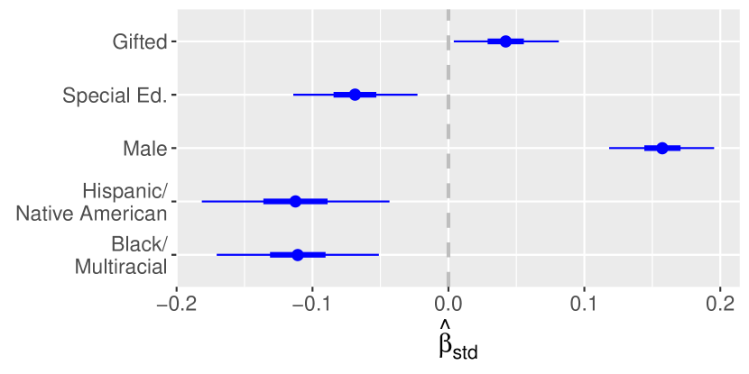
(a)

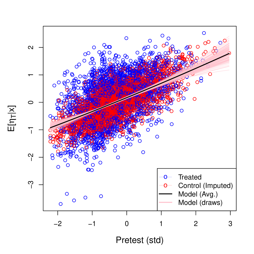
(b)

Figure 4: Fitted model (6.1), predicting $\eta_{T}$. (a) plots estimated coefficients on the categorical variables (race, with reference white/Asian, sex, with reference female, and special education, with reference typical) with 50% and 95% credible intervals. The coefficients represent differences in standard deviations of $\eta_{Ti}$. (b) plots estimated, or imputed, $\eta_{Ti}$ against pretest scores, with the posterior mean quadratic regression line and and 100 random posterior draws.

7.2 CTA1 Treatment Effects

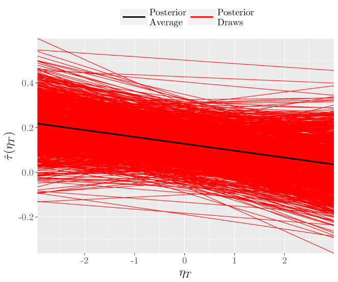
Figure 5: The estimated treatment effect as a function of students’ propensity to master a section, $\mathbb{E}[Y_{T}-Y_{C}|\eta_{T}]$. Red lines are draws from the posterior distribution of the treatment effect function, and the black line is the mean of the posterior.

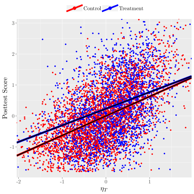
Figure 6: One posterior draw from model (4.1)–(6.3): observed post-test scores $Y$ (pooled standard deviations) as a function of estimated $\eta_{T}$ (in IQR units) in the control and treatment distributions, with regression lines.

Figure 5 displays the posterior mean and posterior draws for the estimated function $\tau(\eta_{T})$. These results suggest that, in fact, the treatment effect decreased with increasing $\eta_{T}$. Students who were more likely to master the sections they worked experienced lower treatment effects. Specifically, a difference of one IQR in $\eta_{T}$ was associated with a reduction of 0.083 in the effect size with a posterior standard deviation of 0.066. In approximately 89% of of the MCMC runs, the slope of $\tau(\eta_{T})$ was negative; a central 95% credible interval for the standardized slope was [-0.212, 0.045].

Why might potential mastery be anticorrelated with treatment effects? Figure 6 plots observed outcomes $Y$ as a function of a posterior draw of the vector $\bm{\eta_{T}}$. (Fortunately, the misspecification apparent in Figure 1, based on $\bar{m}_{T}$ instead of $\eta_{T}$, does not appear here.) There is a positive relationship between $\eta_{T}$ and $Y$ in both treatment groups—students who are more likely to master worked sections tend to score higher on the post-test. However, the slope between $Y$ and $\eta_{T}$ is slightly lower in the treatment group than in the control group. So as $\eta_{T}$ increases, the distance between $Y_{T}$ and $Y_{C}$—the treatment effect—decreases. These results suggest that CTA1 may be more effective for students who would have scored lower on the post-test than for students who would have scored higher. This is unlikely to be the result of ceiling effects, since only one student in the study correctly answered all posttest items. The regression lines in Figure 6 approach each other, but do not cross—the model estimates a positive treatment effect for the entire observed $\eta_{T}$ distribution.

It may seem surprising that our estimate for $\tau(\eta_{T})$ would be more precise than our estimate for $\tau(\bar{m}_{T})$ (Section 3), since $\bar{m}_{T}$ is partially observed, whereas $\eta_{T}$ is completely unobserved. Comparing posterior standard deviations, the slope estimate for $\tau(\eta_{T})$ was roughly twice as precise, after standardizing the units. The model misspecification evident in Figure 1 may be partly to blame. More importantly, both $\bar{m}_{T}$ and $\eta_{T}$ may be thought of as measuring the same latent student quality—the propensity to master a worked section. By employing a more sophisticated and accurate measurement approach, a model based on $\eta_{T}$ will often produce more precise estimates.

8 Model Checking

We checked the fit of model (4.1)–(6.3) in several different ways, using posterior predictive checks (Rubin et al., 1984; Gelman et al., 1996), fitting a series of alternative models, and fitting our main model to fake data, in which the true parameters are known.

This discussion will focus on model checks aimed at two central questions: first, does $\eta_{T}$ indeed measure potential student mastery, and next, can our model successfully estimate real treatment effect functions $\tau(\eta_{T})$ without finding patterns where none exists. A more complete list of model checks and their results is available in the online supplement (Sales and Pane, 2018).

8.1 Checking Measurement Validity

Model 4.1 assumes that students’ propensity to master worked sections is a unidimensional quantity. To test this assumption, we conducted the posterior predictive check described in Levy et al. (2009) using Yen’s $Q_{3}$ discrepancy (Yen, 1993). The median posterior predictive p-value (c.f. Zhu and Stone, 2011) was 0.51, consistent with approximate unidimensionality. Additional details and results can be found in the online supplement (Sales and Pane, 2018).

Another concern is that $\eta_{T}$’s measurement of mastery is confounded with overall student ability. The CTA1 curriculum begins all students at the same place, regardless of their initial ability. Ideally, strong students quickly master more basic sections before progressing to material they find more challenging in advanced sections. On the other hand, weaker students struggle with (and occasionally fail to master) the first set of sections they encounter. If this is the case, one would expect stronger students to achieve mastery more often. To allay this concern, we re-fit the principal stratification model using only data from worked sections in which the student requested at least one hint. This resulted in nearly identical results as our main analysis: a difference of one IQR in $\eta_{T}$ was associated with a decrease of 0.081 in the treatment effect, with a standard error of 0.065.

The online supplement (Sales and Pane, 2018) discusses additional measurement validity checks, including posterior predictive plots, and results from replacing the Rasch model (4.1) with a 2PL or 3PL model. The results were nearly identical to those from our main model—for instance, using a 3PL measurement model, we estimated that a difference of one IQR in $\eta_{T}$ was associated with a decrease of 0.088 in the treatment effect size (SE: 0.068).

8.2 Checking Estimation of $\tau(\eta_{T})$

We fit the model (4.1)–(6.3) to a series of placebo datasets. To create a placebo dataset, we dropped control schools, for which no usage data is available. We simulated a control group by duplicating outcome and covariate data from the treatment group and relabeling the duplicate as the control group. The resulting dataset was comprised of a treatment group and a control group, the former with usage data, but with exactly no treatment effect (since the outcomes in the two groups were identical). We created an additional three datasets by simulating treatment effect functions $\tau(\eta_{T})$ and adding them to the outcomes of the “treated” subjects: a randomly varying treatment effect uncorrelated with $\eta_{T}$, and effects linear and quadratic in $\eta_{T}$. Note that for the last dataset, in which effects are quadratic in $\eta_{T}$, the linear model for $\tau(\eta_{T})$ was misspecified. For these models, we estimated $\eta_{T}$ by fitting (4.1)–(6.1) to usage data from the treatment group.

The results of fitting our model to these four datasets—one with no treatment effect and three with simulated effects—are displayed in Figure 7. In the first three datasets, for which our treatment effect model was well-specified, the model’s estimates are in line with the truth. In the final placebo dataset, in which the model was misspecified, while the linear estimate of $\tau(\eta_{T})$ fails to capture the true pattern, it does lead to the correct conclusion of little or no linear correlation between treatment effects and $\eta_{T}$.

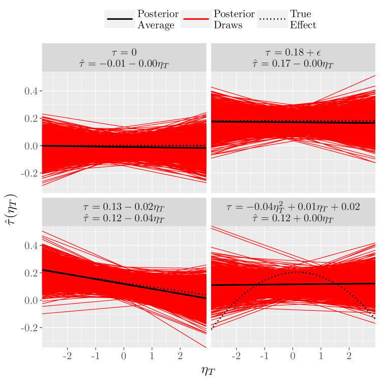
Figure 7: Treatment effect estimates when model (4.1)–(6.3) was fit to datasets with simulated treatment effects, as described in Section 8.2. In each figure, the solid black line represents the true treatment effect, the dotted line is the posterior mean of $b_{1}$, and the red lines are draws from the posterior distribution. The true and estimated (posterior mean) treatment effect functions are shown at the top of each panel. Clockwise from the upper left, there is no treatment effect, a random treatment effect uncorrelated with $\eta_{T}$, a treatment effect linear in $\eta_{T}$ and a treatment effect quadratic in $\eta_{T}$.

9 Discussion

9.1 The Role of Mastery in the Cognitive Tutor

Were mastery learning the only driver of CTA1 effectiveness, we would expect effectiveness to correlate with students’ potential section mastery. In fact, the opposite seems to be the case—average effects appear to decrease with students’ mastery propensity (though they remain positive throughout).

On the other hand, $\eta_{T}$, the latent parameter measuring mastery propensity, positively correlates with students’ pre- and post-test scores in both treatment groups. Students who were more likely to master worked sections were stronger at the at the beginning of the year and knew more Algebra I at the end of the year. If the CTA1 effect were larger for lower performing students than for stronger students we would expect to see a negative correlation between $\eta_{T}$ and treatment effects. Similarly, a wide range of pre-treatment student characteristics, both measured and unmeasured, may explain the observed relationship between $\eta_{T}$ and treatment effects.

Future work will extend this analysis to the middle school arm of the study. Middle school algebra students are not only younger than those in our high-school sample, but are higher achieving as well, on average, adding an interesting dimension to this analysis. However, Pane et al. (2014) reported an imbalance in pretest scores of treatment and control middle school students, suggesting that assignment to the treatment condition may have influenced which students chose to take algebra in middle school instead of waiting until high school. This apparent selection into the treatment condition would have to be accounted for in a principal stratification model, adding an additional modeling challenge beyond those described here.

From a practical standpoint, these results are encouraging. Fortunately, there is no evidence here that students’ occasional failure to master worked sections seriously impedes CTA1’s effectiveness. In fact, students who are more likely to wheel-spin may benefit even more from CTA1 than their more successful peers. Struggling students, who are less likely to achieve mastery, are also most in need of help. The results here suggest that the Cognitive Tutor is not failing them.

9.2 Latent Variables in a Potential Outcomes Framework

In the course of modeling data from the CTA1 experiment, it became necessary to introduce a latent variable into principal stratification modeling. We are unaware of this being done previously. Latent variables are necessary here because directly observable statistics ostensibly measuring student mastery—such as $\bar{m}$— were woefully inadequate. In particular, $\bar{m}$ does not account for which, or how many, sections students attempted. On the other hand, IRT provides a wealth of models and a mature statistical theory for modeling student mastery potential. Operationalizing students’ potential mastery via the Rasch parameter $\eta_{T}$ has clear advantages over the simpler approaches previously available.

That said, there may be some tension between latent variables and the Rubin Causal Model, on which principal stratification is based. For instance, Imbens and Rubin (1997, p. 306) wrote:

Inferences across models with different parametric structures can be compared directly because these inferences are all driven by the posterior predictive distribution of the same causal estimands defined by the potentially observable outcomes.

One of the central arguments for the Rubin Causal Model is that its target estimand is defined in a way that is independent of the model used to estimate it. In contrast, the definition of the parameter $\eta_{T}$ is inherently tied to the Rasch model (4.1)–(6.1).

But latent variables are themselves measurements. The only difference between measurement via latent variables versus via other measurement tools used in principal stratification is that the measurement takes place within the principal stratification model. Perhaps the most common outcome in causal education research is test scores, themselves typically calculated with an IRT model—in other words, latent variables. The models that give rise to the test scores are fit separately from the causal model, giving them the appearance of objective measurements. Similarly, an analyst could fit model (4.1)–(6.1) to mastery and covariate data without reference to outcomes, principal strata, or causal inference at all. Including the measurement model as a component of the larger causal model is good statistical practice.

However, especially given the difficulty of fitting even much simpler principal stratification models, an abundance of caution is in order. Theory and guidance regarding when latent variable principal stratification models will give accurate answers would be particularly helpful. The role of covariates in predicting latent variable values—and hence imputing them for control subjects—is particularly pressing.

With the foundation set, latent variable principal stratification can open many doors. For instance, researchers may be able to use cluster analysis techniques to summarize large numbers of intermediate variables, and then examine treatment effect heterogeneity between clusters. Factor analysis may play a similar role in continuous principal stratification. Latent variable principal stratification has the potential to facilitate more—and more nuanced—scientific discoveries.

References

- Anderson et al. [1985] John R Anderson, C Franklin Boyle, and Brian J Reiser. Intelligent tutoring systems. Science(Washington), 228(4698):456–462, 1985.
- Anderson et al. [1995] John R Anderson, Albert T Corbett, Kenneth R Koedinger, and Ray Pelletier. Cognitive tutors: Lessons learned. The journal of the learning sciences, 4(2):167–207, 1995.
- Bates et al. [2015] Douglas Bates, Martin Mächler, Ben Bolker, and Steve Walker. Fitting linear mixed-effects models using lme4. Journal of Statistical Software, 67(1):1–48, 2015. 10.18637/jss.v067.i01.
- Beck and Gong [2013] Joseph E Beck and Yue Gong. Wheel-spinning: Students who fail to master a skill. In International Conference on Artificial Intelligence in Education, pages 431–440. Springer, 2013.
- Bloom [1968] Benjamin S Bloom. Learning for mastery. instruction and curriculum. regional education laboratory for the carolinas and virginia, topical papers and reprints, number 1. Evaluation comment, 1(2):n2, 1968.
- Bowers et al. [2017] Jake Bowers, Mark Fredrickson, and Ben Hansen. RItools: Randomization Inference Tools (Development Version), 2017. URL https://github.com/markmfredrickson/RItools. R package version 0.2-0.
- Carroll et al. [2006] Raymond J Carroll, David Ruppert, Leonard A Stefanski, and Ciprian M Crainiceanu. Measurement error in nonlinear models: a modern perspective. CRC press, 2006.
- De Boeck and Wilson [2013] Paul De Boeck and Mark Wilson. Explanatory item response models: A generalized linear and nonlinear approach. Springer Science & Business Media, 2013.
- Efron and Morris [1973] Bradley Efron and Carl Morris. Stein’s estimation rule and its competitors—an empirical bayes approach. Journal of the American Statistical Association, 68(341):117–130, 1973.
- Embretson and Reise [2013] Susan E Embretson and Steven P Reise. Item response theory for psychologists. Psychology Press, 2013.
- Feller et al. [2016a] Avi Feller, Evan Greif, Luke Miratrix, and Natesh Pillai. Principal stratification in the twilight zone: Weakly separated components in finite mixture models. arXiv preprint arXiv:1602.06595, 2016a.
- Feller et al. [2016b] Avi Feller, Todd Grindal, Luke Miratrix, Lindsay C Page, et al. Compared to what? variation in the impacts of early childhood education by alternative care type. The Annals of Applied Statistics, 10(3):1245–1285, 2016b.
- Frangakis and Rubin [2002] Constantine E Frangakis and Donald B Rubin. Principal stratification in causal inference. Biometrics, 58(1):21–29, 2002.
- Gelman and Hill [2006] Andrew Gelman and Jennifer Hill. Data analysis using regression and multilevel/hierarchical models. Cambridge university press, 2006.
- Gelman and Rubin [1992] Andrew Gelman and Donald B Rubin. Inference from iterative simulation using multiple sequences. Statistical science, pages 457–472, 1992.
- Gelman et al. [1996] Andrew Gelman, Xiao-Li Meng, and Hal Stern. Posterior predictive assessment of model fitness via realized discrepancies. Statistica sinica, pages 733–760, 1996.
- Gelman et al. [2014] Andrew Gelman, John B Carlin, Hal S Stern, David B Dunson, Aki Vehtari, and Donald B Rubin. Bayesian data analysis, volume 2. CRC press Boca Raton, FL, 2014.
- Gilbert and Hudgens [2008] Peter B Gilbert and Michael G Hudgens. Evaluating candidate principal surrogate endpoints. Biometrics, 64(4):1146–1154, 2008.
- Griffin et al. [2008] Beth Ann Griffin, Daniel F McCaffery, and Andrew R Morral. An application of principal stratification to control for institutionalization at follow-up in studies of substance abuse treatment programs. The annals of applied statistics, 2(3):1034, 2008.
- Imbens and Rubin [1997] Guido W Imbens and Donald B Rubin. Bayesian inference for causal effects in randomized experiments with noncompliance. The Annals of Statistics, pages 305–327, 1997.
- Israni et al. [2018] Anita Israni, Adam C Sales, and John F Pane. Mastery learning in practice: A (mostly) descriptive analysis of log data from the cognitive tutor algebra i effectiveness trial, 2018.
- Jin and Rubin [2008] Hui Jin and Donald B Rubin. Principal stratification for causal inference with extended partial compliance. Journal of the American Statistical Association, 103(481):101–111, 2008.
- Kalton [1968] Graham Kalton. Standardization: A technique to control for extraneous variables. Applied Statistics, pages 118–136, 1968.
- Kulik et al. [1990] Chen-Lin C Kulik, James A Kulik, and Robert L Bangert-Drowns. Effectiveness of mastery learning programs: A meta-analysis. Review of educational research, 60(2):265–299, 1990.
- Levy et al. [2009] Roy Levy, Robert J Mislevy, and Sandip Sinharay. Posterior predictive model checking for multidimensionality in item response theory. Applied Psychological Measurement, 33(7):519–537, 2009.
- Li et al. [2015] Fan Li, Alessandra Mattei, Fabrizia Mealli, et al. Evaluating the causal effect of university grants on student dropout: evidence from a regression discontinuity design using principal stratification. The Annals of Applied Statistics, 9(4):1906–1931, 2015.
- Little and Rubin [2014] Roderick JA Little and Donald B Rubin. Statistical analysis with missing data. John Wiley & Sons, 2014.
- Mattei et al. [2013] Alessandra Mattei, Fan Li, Fabrizia Mealli, et al. Exploiting multiple outcomes in bayesian principal stratification analysis with application to the evaluation of a job training program. The Annals of Applied Statistics, 7(4):2336–2360, 2013.
- Miratrix et al. [2017] Luke Miratrix, Jane Furey, Avi Feller, Todd Grindal, and Lindsay C Page. Bounding, an accessible method for estimating principal causal effects, examined and explained. Journal of Research on Educational Effectiveness, pages 1–30, 2017.
- Neyman [1923] Jersey Neyman. Sur les applications de la théorie des probabilités aux experiences agricoles: Essai des principes. Roczniki Nauk Rolniczych, 10:1–51, 1923.
- Nolen and Hudgens [2011] Tracy L Nolen and Michael G Hudgens. Randomization-based inference within principal strata. Journal of the American Statistical Association, 106(494):581–593, 2011.
- Page [2012] Lindsay C Page. Principal stratification as a framework for investigating mediational processes in experimental settings. Journal of Research on Educational Effectiveness, 5(3):215–244, 2012.
- Pane et al. [2014] John F Pane, Beth Ann Griffin, Daniel F McCaffrey, and Rita Karam. Effectiveness of cognitive tutor algebra i at scale. Educational Evaluation and Policy Analysis, 36(2):127–144, 2014.
- R Core Team [2016] R Core Team. R: A Language and Environment for Statistical Computing. R Foundation for Statistical Computing, Vienna, Austria, 2016. URL https://www.R-project.org/.
- Rasch [1993] Georg Rasch. Probabilistic models for some intelligence and attainment tests. ERIC, 1993.
- Richardson et al. [2011] Thomas S Richardson, Robin J Evans, and James M Robins. Transparent parameterizations of models for potential outcomes. Bayesian Statistics, 9:569–610, 2011.
- Rubin [1978] Donald B Rubin. Bayesian inference for causal effects: The role of randomization. The Annals of statistics, pages 34–58, 1978.
- Rubin [1980] Donald B Rubin. Discussion of “randomization analysis of experimental data: The fisher randomization test”. Journal of the American Statistical Association, 75(371):591–593, 1980.
- Rubin [1981] Donald B Rubin. Estimation in parallel randomized experiments. Journal of Educational Statistics, 6(4):377–401, 1981.
- Rubin et al. [1984] Donald B Rubin et al. Bayesianly justifiable and relevant frequency calculations for the applied statistician. The Annals of Statistics, 12(4):1151–1172, 1984.
- Sales and Pane [2018] Adam C Sales and John F Pane. Supplement to: “the role of mastery learning in intelligent tutoring systems: Principal stratification on a latent variable”, 2018. web supplement.
- Sales et al. [2016] Adam C Sales, Asa Wilks, and John F Pane. Student usage predicts treatment effect heterogeneity in the cognitive tutor algebra i program. In Proceedings of the 9th International Conference on Educational Data Mining. International Educational Data Mining Society, pages 207–214, 2016.
- Schwartz et al. [2011] Scott L Schwartz, Fan Li, and Fabrizia Mealli. A bayesian semiparametric approach to intermediate variables in causal inference. Journal of the American Statistical Association, 106(496):1331–1344, 2011.
- Stan Development Team [2016] Stan Development Team. RStan: the R interface to Stan, 2016. URL http://mc-stan.org/. R package version 2.14.1.
- Stekhoven and Buehlmann [2012] Daniel J. Stekhoven and Peter Buehlmann. Missforest - non-parametric missing value imputation for mixed-type data. Bioinformatics, 28(1):112–118, 2012.
- Sterne et al. [2009] Jonathan AC Sterne, Ian R White, John B Carlin, Michael Spratt, Patrick Royston, Michael G Kenward, Angela M Wood, and James R Carpenter. Multiple imputation for missing data in epidemiological and clinical research: potential and pitfalls. Bmj, 338:b2393, 2009.
- van der Linden and Hambleton [2013] Wim J van der Linden and Ronald K Hambleton. Handbook of modern item response theory. Springer Science & Business Media, 2013.
- Yen [1993] Wendy M Yen. Scaling performance assessments: Strategies for managing local item dependence. Journal of educational measurement, 30(3):187–213, 1993.
- Zhu and Stone [2011] Xiaowen Zhu and Clement A Stone. Assessing fit of unidimensional graded response models using bayesian methods. Journal of Educational Measurement, 48(1):81–97, 2011.