Moving obstacle potential in a spin-orbit-coupled Bose-Einstein condensate

Abstract

We investigate the dynamics around an obstacle potential moving in the plane-wave state of a pseudospin-$1/2$ Bose-Einstein condensate with Rashba spin-orbit coupling. We numerically investigate the dynamics of the system and find that it depends not only on the velocity of the obstacle but also significantly on the direction of obstacle motion, which are verified by a Bogoliubov analysis. The excitation diagram with respect to the velocity and direction is obtained. The dependence of the critical velocity on the strength of the spin-orbit coupling and the size of the obstacle is also investigated.

I Introduction

The successful experimental realization of various synthetic gauge fields and spin-orbit coupling (SOC) in Bose-Einstein condensates (BECs) has recently drawn considerable theoretical attention Y.-J. Lin1 ; Y.-J. Lin2 ; Y.-J. Lin3 ; Y.-J. Lin4 ; B. M. Anderson ; Z. Fu ; S. C. Ji0 ; L. Huang ; Z. M. Meng ; Z. Wu , with a number of studies addressing the ground state structures and static properties of topological excitations (for recent reviews, see, for example, Refs. J. Dalibard ; N. Goldman ; H. Zhai0 ). Such synthetic gauge potentials in cold atoms are powerful tools for quantum many-body simulators of real materials. Moreover, the spin-orbit-coupled (SO-coupled) BEC exhibits numerous novel phases that cannot be found in conventional condensed matter systems.

In the present paper, we focus on the problem of the moving obstacle potential in an SO-coupled BEC. The drag force on a moving impurity in a SO-coupled BEC has been calculated using the Bogoliubov spectrum P.-S. He ; R. Liao . In contrast, we directly solve the Gross-Pitaevskii (GP) equation with SOC and investigate the dynamical effects of the moving obstacle potential on the SO-coupled condensate. Most theoretical studies on BEC with Rashba SOC have focused on the static properties of the condensate C. Wang ; T. L. Ho ; X.-F. Zhou ; S. Sinha ; H. Hu ; T. Kawakami ; B. Ramachandhran , and there have only been a few studies on dynamics J. Radic ; A. L. Fetter ; K. Kasamatsu ; A. Gallem .

The Dynamics of an SO-coupled BEC around a moving obstacle potential differs significantly from that of the usual scalar BEC in two ways. First, the ground state of the SO-coupled BEC breaks rotational symmetry, and the excitation spectrum above the ground state has an anisotropic characteristic form with a roton minimum Q. Zhu ; M. A. Khamehchi ; S. C. Ji ; K. Sun . Because of this feature, the Landau critical velocity and excitation properties depend on the direction of obstacle motion. Second, due to the close relationship between the spin and motional degrees of freedom, the dynamic properties of quantized vortices and solitons are dramatically altered by the SOC M. Kato . Consequently, the generation of vortices and waves around the moving obstacle potential is significantly affected by the SOC.

The remainder of the present paper is organized as follows. In Sec. II, we formulate the theoretical model for a moving obstacle potential in a uniform SO-coupled BEC. In Sec. III, the excitation dynamics induced by the obstacle potential and the Bogoliubov analysis are presented. The parameter dependence and velocity field are investigated in Secs. IV and V, respectively. Finally, in Sec. VI, the main results of the present paper are summarized.

II Formulation of the problem

We consider a BEC of quasispin-$1/2$ atoms with Rashba SOC, where an obstacle potential is moving in a uniform system. The mean-field approximation is used, and the dynamics of the system is described by the GP equation as follows:

$$i\hbar\frac{\partial}{\partial t}\bm{\Psi}=-\frac{\hbar^{2}}{2m}\bm{\nabla}^{2}\bm{\Psi} + i\frac{\hbar k_{0}}{m}\bm{\nabla}\cdot\bm{\sigma}_{\perp}\bm{\Psi}$$ (1)

$$+ U(\bm{r},t)\bm{\Psi}+\hat{G}\left(\bm{\Psi},\bm{\Psi}^{\dagger}\right)\bm{\Psi},$$

where $\bm{\Psi}(\bm{r})=(\psi_{1}(\bm{r}),\psi_{2}(\bm{r}))^{T}$ is the spinor order parameter, $m$ is the mass of atoms, $k_{0}$ is the SOC coefficient, $\bm{\sigma}_{\perp}=(\sigma_{x},\sigma_{y},0)$ are $2\times 2$ Pauli matrices, and $U(\bm{r},t)$ is a moving obstacle potential. The interaction matrix in Eq. (1) is given by

$$\hat{G}(\bm{\Psi},\bm{\Psi}^{\dagger})=\begin{pmatrix}\textmd{g}_{0}|\psi_{1}|^{2}&\textmd{g}_{12}|\psi_{2}|^{2}\\ \textmd{g}_{12}|\psi_{1}|^{2}&\textmd{g}_{0}|\psi_{2}|^{2}\end{pmatrix},$$ (2)

where $\textmd{g}_{0}$ and $\textmd{g}_{12}$ are the intra- and inter-component interaction coefficients, respectively. (Here, we further assume that the two intracomponent interaction parameters are the same.) We consider an infinite system in which the atomic density $\bm{\Psi}^{\dagger}\bm{\Psi}$ far from the potential is constant, $n_{0}$. In the following, we normalize the length and time by the healing length $\xi=\hbar/(\textmd{g}_{0}n_{0}m)$ and the characteristic time scale $\tau=\hbar/(\textmd{g}_{0}n_{0})$. In this unit, the wave function, velocity, and energy are normalized by $n_{0}$, $\sqrt{\textmd{g}_{0}n_{0}/m}$, and $\textmd{g}_{0}n_{0}$. We transform Eq. (1) into a frame of reference that moves with the potential at velocity $\bm{v}=(v\cos\theta_{v},v\sin\theta_{v})$. The normalized GP equation becomes

$$i\frac{\partial\psi_{1}}{\partial t}=-\frac{1}{2}\bm{\nabla}^{2}\psi_{1}+i\kappa\partial_{-}\psi_{2}+i\bm{v}\cdot\bm{\nabla}\psi_{1}$$

$$+V(\bm{r})\psi_{1}+\left(|\psi_{1}|^{2}+\gamma|\psi_{2}|^{2}\right)\psi_{1},$$ (3a)

$$i\frac{\partial\psi_{2}}{\partial t}=-\frac{1}{2}\bm{\nabla}^{2}\psi_{2}+i\kappa\partial_{-}\psi_{1}+i\bm{v}\cdot\bm{\nabla}\psi_{2}$$

$$+V(\bm{r})\psi_{2}+\left(\gamma|\psi_{1}|^{2}+|\psi_{2}|^{2}\right)\psi_{2},$$ (3b)

where $\partial_{\pm}=\partial/\partial x\pm i\partial/\partial y$, $\kappa=k_{0}/\sqrt{g_{0}n_{0}m}$, and $\gamma=\textmd{g}_{12}/\textmd{g}_{0}$. We use a circular potential with radius $R$ as

$$V(\bm{r})=\begin{cases}V_{0}&(|\bm{r}|\leq R)\\ 0&(|\bm{r}|>R),\end{cases}$$ (4)

where the potential height $V_{0}$ is taken to be much larger than the chemical potential.

The ground state without the potential is the plane-wave state for $\gamma<1$ and the stripe state for $\gamma>1$. In the following discussion, we focus on the miscible case, $\gamma<1$, and the ground state far from the potential is given by the plane-wave state, as follows:

$$\bm{\Psi}(\bm{r})=\frac{1}{\sqrt{2}}\left(\begin{array}[]{c}e^{i\kappa x}\\ e^{i\kappa x}\end{array}\right),$$ (5)

where the wave vector is chosen to be in the $x$ direction.

We numerically solve Eq. (3) by the pseudospectral method using the fourth-order Runge-Kutta scheme. The initial state is the ground state with $\bm{v}=0$, which is the plane-wave state in Eq. (5) far from the potential. The initial state is prepared by the imaginary-time propagation method, in which $i$ on the left-hand side of Eq. (3) is replaced with $-1$. The numerical space is taken to be $400\times 400$, which is sufficiently large, and the effect of the periodic boundary condition can be neglected.

III Excitation induced by an obstacle

III.1 Dynamics of the system

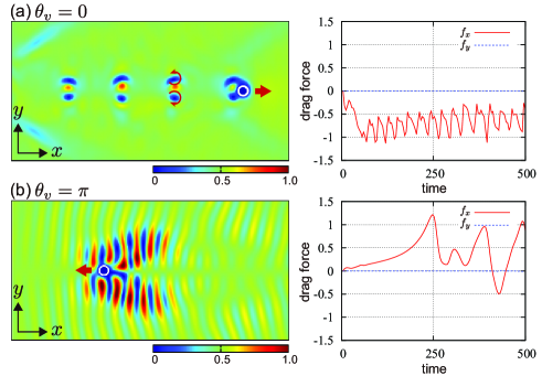
Figure 1: Typical snapshots of the density distribution $|\psi_{1}|^{2}$ and time evolution of the drag force $\bm{f}$ exerted on the potential. The velocities of the potential $(v,\theta_{v})$ are (a) $(0.5,0)$ and (b) $(0.05,\pi)$. The field of view of the left-hand panels is $60\times 30$. The white circles represent the obstacle potential, and the thick arrows indicate the moving direction. The curved arrows indicate the directions of the circulations of the vortices. The parameters are $R=0.5$, $\kappa=1$, and $\gamma=0.8$. See the Supplemental Material for movies of the dynamics of component 1 SM .

First, we focus on the two special cases of $\theta_{v}=0$ and $\theta_{v}=\pi$, where $\theta_{v}$ is the angle between the obstacle velocity $\bm{v}$ and the $x$ axis. In the case of $\theta_{v}=0$, when the velocity $v$ exceeds a critical value, vortex-antivortex pairs are created, as shown in the left-hand panel of Fig. 1(a). In this case, the periodic generation of vortex-antivortex pairs is, in a sense, reminiscent of the scalar case. However, the created vortex pairs are different from those in the scalar BEC, in that the vortex cores in both components deviate from each other, producing pairs of half-quantum vortices M. Kato . The right-hand panel of Fig. 1(a) shows the drag force experienced by the obstacle, defined by $\bm{f}_{\rm d}=i\partial_{t}\int d\bm{r}(\Psi^{\dagger}\bm{\nabla}\Psi)$. The drag force in the $x$ direction exhibits periodic oscillation due to the periodic generation of vortices, whereas the drag force in the $y$ direction remains zero. In the case of $\theta_{v}=\pi$, when the velocity $v$ exceeds a critical velocity, spin waves are excited, as shown in the left-hand panel of Fig. 1(b), which is very different from the case of $\theta_{v}=0$. In this spin-wave state, high-density regions of components 1 and 2 are alternately aligned, as in the stripe state of an SOC BEC. The critical velocity of the spin-wave generation is much smaller than that of the vortex generation for $\theta_{v}=0$. Thus, the excitation dynamics is strongly anisotropic with respect to the moving obstacle potential.

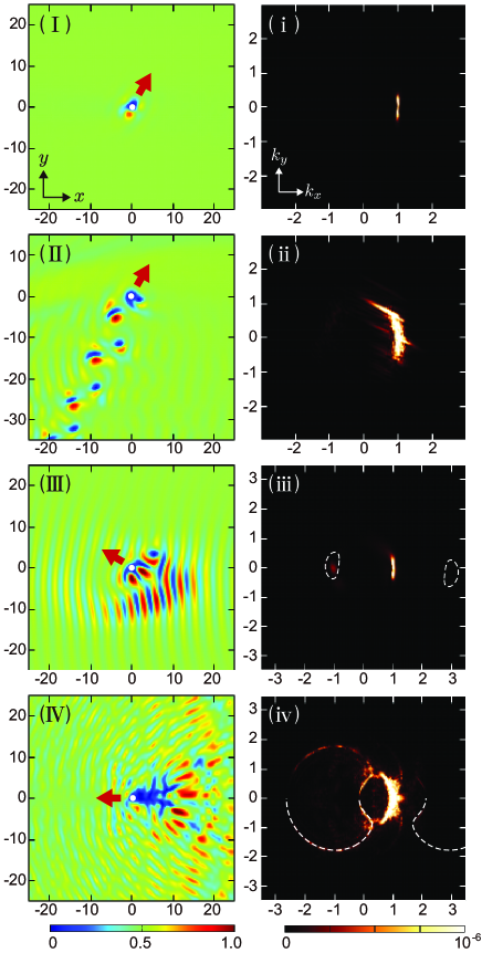
Figure 2: Snapshots of (I)-(IV) the density distributions $|\psi_{1}|^{2}$ and (i)-(iv) the momentum-space distribution $|\tilde{\psi}_{1}|^{2}$ for $\kappa=1$, $\gamma=0.8$, and $R=0.5$, where $\tilde{\psi}_{1}$ is the Fourier transform of $\psi_{1}$. (I, i) $(v,\theta_{v})=(0.1,\pi/3)$, (II, ii) $(v,\theta_{v})=(0.2,\pi/3)$, (III, iii) $(v,\theta_{v})=(0.07,5\pi/6)$, and (IV, iv) $(v,\theta_{v})=(0.4,\pi)$. The white solid circles and the red arrows in the left-hand panels are the obstacle potentials and moving directions, respectively. The dashed lines in (iii) and (iv) indicate the analytical solutions of $\omega(k_{x}-\kappa,k_{y})=0$ in Eq. (12). (In (iv), the dashed lines are shown only for $k_{y}<0$.) See the Supplemental Material for movies of the dynamics of $|\psi_{1}|^{2}$ and $|\tilde{\psi}_{1}|^{2}$ SM .

For a deeper understanding of the anisotropic properties, we explore the $v$ and $\theta_{v}$ dependence of the dynamics. Figure 2 shows four typical dynamics with different velocities and azimuthal angles of the obstacle motion. These four kinds of dynamics are (I) weak excitation, (II) vortex pairs, (III) spin wave, and (IV) strong excitation. In the absence of excitation, the momentum-space distribution is $\delta(k_{x}-\kappa,k_{y})$ due to the plane-wave background. For the weak excitation, no pronounced excitations are observed in the density distributions, but the long wavelength excitations are induced at $k_{x}=\kappa$ and $|k_{y}|\lesssim 0.4$, as shown in Fig. 2(i). For the spin wave, we find excitations at $\bm{k}\simeq-\kappa\bm{e}_{x}$, as shown in Fig. 2(iii). For the strong excitation, the shock-wave pattern appears in the density distribution, as shown in Fig. 2(IV), which has a ring shape in the momentum space, as shown in Fig. 2(iv). These momentum-space behaviors are explained in Sec. III.2.

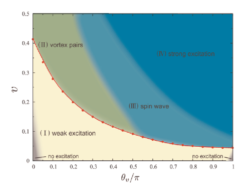
Figure 3: The excitation diagram with respect to $v$ and $\theta_{v}$ for $\kappa=1$, $\gamma=0.8$, and $R=0.5$. The dynamics are classified into (I)-(IV), which correspond to those in Fig. 3. The red points indicate the critical velocity, at which the drag force increases suddenly, and the red line is a visual guide.

Figure 3 shows a diagram of the four kinds of excitation with respect to $v$ and $\theta_{v}$, where regions (I)-(IV) correspond to the dynamics in Fig. 2. As $v$ and $\theta_{v}$ are increased, the excitation behavior changes from (II) to (IV). The boundaries between these three regions are vague. In contrast, there is a sharp boundary between region (I) and regions (II)-(IV), as indicated by the red points in Fig. 3. When we start from region (I) and slowly increase the velocity $v$, the small drag force in region (I) steeply increases at this boundary. For small $v$ and $\theta\simeq 0,\pi$, there are narrow regions in which the drag force almost vanishes, which are indicated by the dark regions in Fig. 3.

III.2 Bogoliubov analysis

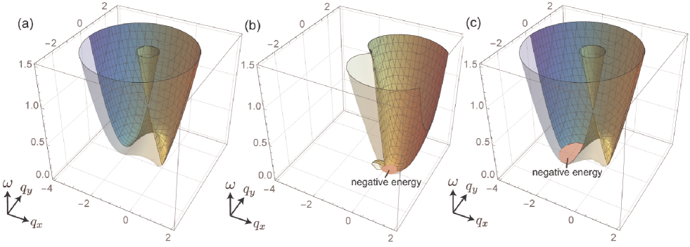
Figure 4: Excitation spectrum of a uniform system for $\kappa=1$ and $\gamma=0.8$ in the frame moving at velocities (a) $(v,\theta_{v})=(0,0)$, (b) $(v,\theta_{v})=(1,0)$, and (c) $(v,\theta_{v})=(0.1,\pi)$. The colored regions on the $q_{x}$-$q_{y}$ plane indicate negative energy, $\omega(\bm{q})<0$.

We perform a Bogoliubov analysis in order to clarify the numerically obtained behavior. The wave function can be written as

$$\bm{\Psi}(\bm{r},t)=e^{-i\mu t+i\kappa x}\left[\frac{1}{\sqrt{2}}\left(\begin{array}[]{c}1\\ 1\end{array}\right)+\bm{\delta}\bm{\Psi}(\bm{r},t)\right],$$ (6)

where $\mu=-\kappa^{2}/2-v_{x}\kappa+(1+\gamma)/2$ is the chemical potential. The small excitation $\delta\bm{\Psi}(\bm{r},t)$ is decomposed into

$$\delta\bm{\Psi}(\bm{r},t)=\bm{\alpha}e^{i(\bm{q}\cdot\bm{r}-\omega t)}+\bm{\beta}^{\ast}e^{-i(\bm{q}\cdot\bm{r}-\omega t)},$$ (7)

where $\bm{\alpha}=(\alpha_{1},\alpha_{2})^{\rm T}$ and $\bm{\beta}=(\beta_{1},\beta_{2})^{\rm T}$ are the amplitudes, $\bm{q}=(q\cos\theta_{q},q\sin\theta_{q})$ is the wave number, and $\omega$ is the frequency of the excitation. Substituting Eq. (6) into Eq. (3) with $V=0$ and taking the first order of $\delta\bm{\Psi}$, we obtain

$$\left(\mu^{\prime}+i\frac{\partial}{\partial t}\right)\delta\bm{\Psi}=(\mathcal{H}_{0}+\mathcal{H}_{1})\delta\bm{\Psi}+\mathcal{H}_{2}\delta\bm{\Psi}^{\ast}+i\bm{v}\cdot\nabla\delta\bm{\Psi},$$ (8)

where $\mu^{\prime}=-\kappa^{2}/2+(1+\gamma)/2$,

$$\mathcal{H}_{0}=\begin{pmatrix}-\frac{1}{2}(\bm{\nabla}+i\kappa\bm{e}_{x})^{2}&i\kappa\partial_{-}-\kappa^{2}\\ i\kappa\partial_{+}-\kappa^{2}&-\frac{1}{2}(\bm{\nabla}+i\kappa\bm{e}_{x})^{2}\end{pmatrix},$$ (9)

and

$$\mathcal{H}_{1}=\frac{1}{2}\begin{pmatrix}2+\gamma&\gamma\\ \gamma&2+\gamma\end{pmatrix},\mathcal{H}_{2}=\frac{1}{2}\begin{pmatrix}1&\gamma\\ \gamma&1\end{pmatrix}.$$ (10)

The Bogoliubov equation is obtained from Eqs. (7)-(10) as $\{\mathcal{H}(\bm{q})-[\omega(\bm{q})+\bm{v}\cdot\bm{q}]\mathcal{I}\}\bm{\chi}=\bm{0}$, where

$$\mathcal{H}(\bm{q})=\begin{pmatrix}\frac{1}{2}q^{2}+\kappa q_{x}+\kappa^{2}+\frac{1}{2}&-\kappa q_{-}-\kappa^{2}+\frac{1}{2}\gamma&\frac{1}{2}&\frac{1}{2}\gamma\\ -\kappa q_{+}-\kappa^{2}+\frac{1}{2}\gamma&\frac{1}{2}q^{2}+\kappa q_{x}+\kappa^{2}+\frac{1}{2}&\frac{1}{2}\gamma&\frac{1}{2}\\ -\frac{1}{2}&-\frac{1}{2}\gamma&-\frac{1}{2}q^{2}+\kappa q_{x}-\kappa^{2}-\frac{1}{2}&-\kappa q_{+}+\kappa^{2}-\frac{1}{2}\gamma\\ -\frac{1}{2}\gamma&-\frac{1}{2}&-\kappa q_{-}+\kappa^{2}-\frac{1}{2}\gamma&-\frac{1}{2}q^{2}+\kappa q_{x}-\kappa^{2}-\frac{1}{2}\end{pmatrix}$$ (11)

and $\bm{\chi}=(\alpha_{1},\alpha_{2},\beta_{1},\beta_{2})^{\rm T}$. The Bogoliubov excitation spectrum $\omega(\bm{q},\bm{v})$ is the solution of

$$|\mathcal{H}(\bm{q})-(\omega+\bm{v}\cdot\bm{q})\mathcal{I}|=0.$$ (12)

Figure 4(a) shows the excitation spectrum $\omega(\bm{q},\bm{v})$ at $\bm{v}=\bm{0}$. The spectrum breaks the rotational symmetry and has a roton-like minimum at $q_{y}<0$. For nonzero $v$, a region in which $\omega$ becomes negative appears. The Landau critical velocity is defined as the velocity above which the negative-$\omega$ region appears on the $q_{x}$-$q_{y}$ plane. Thus, in the present case, the Landau critical velocity depends on the angle $\theta_{v}$ of the moving potential. When $\theta_{v}=0$, the negative-energy region is located near the origin of the momentum space, as shown in Fig. 4(b), which is similar to the case of a scalar BEC. For $\theta_{v}=\pi$, on the other hand, the negative-energy region appears at finite momentum due to the roton-like minimum, as shown in Fig. 4(c). This corresponds to the spin-wave excitation in Figs. 2(III) and 2(iii).

Setting $\omega=0$ in Eq. (12), we have

$$|\mathcal{H}(\bm{q})-\bm{v}\cdot\bm{q}\mathcal{I}|=0.$$ (13)

For given $\theta_{v}$, the Landau critical velocity $v_{L}$ is the minimum value of $v\geq 0$ for which Eq. (13) has at least a real solution $\bm{q}$. First, we solve Eq. (13) under the assumption that the solution is $q\simeq 0$. Taking the limit $q\rightarrow 0$, Eq. (13) is rewritten as

$$v=\sqrt{\frac{1+\gamma}{2}}\left|\frac{\cos\theta_{q}}{\cos(\theta_{q}-\theta_{v})}\right|,$$ (14)

where $\theta_{q}$ is the azimuthal angle in the $q_{x}$-$q_{y}$ plane. When $\theta_{v}\neq 0$ and $\theta_{v}\neq\pi$, the minimum value of $v\geq 0$ for which Eq. (14) has a solution is $v=0$ (the solution is $\theta_{q}=\pm\pi/2$). Thus, the Landau critical velocity for $\theta_{v}\neq 0$ and $\theta_{v}\neq\pi$ is $v_{L}=0$. The instability around $\theta_{q}=\pm\pi/2$ appears in Fig. 2(i). The Landau critical velocities for $\theta_{v}=0$ and $\theta_{v}=\pi$ are obtained analytically, and we have

$$v_{L}(\theta_{v})=\begin{cases}\sqrt{(1+\gamma)/2}&(\theta_{v}=0)\\ -\kappa+\sqrt{\kappa^{2}+(1-\gamma)/2}&(\theta_{v}=\pi)\\ 0&({\rm other})\end{cases}.$$ (15)

Note that $v_{L}$ for $\theta_{v}=0$ is independent of $\kappa$, which has a phonon-like relation $\omega\propto q_{x}$ for $q_{x}\ll 1$, as in the Bogoliubov mode of a scalar BEC. When $\theta_{v}=\pi$, the wave number

$$q_{x}=-\sqrt[4]{8\kappa^{2}(1-\gamma+2\kappa^{2})}$$ (16)

first becomes negative above the Landau critical velocity, which corresponds to the wave number for the spin wave shown in Figs. 2(III) and 2(iii). In the limit of $\kappa\rightarrow 0$, the two velocities in Eq. (15) are $\sqrt{(1\pm\gamma)/2}$, which agree with those in the two-component BEC without SO coupling.

Although the Landau critical velocity is 0 for $\theta_{v}\neq 0$ and $\theta_{v}\neq\pi$ in Eq. (15), the effect of the excitation remains slight when $v$ is small, as shown in Figs. 2(I) and 2(i). However, there exists an effective critical velocity, above which the drag force suddenly increases, as indicated by the red line in Fig. 3.

The dashed lines in Figs. 2(iii) and 2(iv) indicate the analytical solutions of $\omega(k_{x}-\kappa,k_{y},\bm{v})=0$ for $(v,\theta_{v})=(0.07,5\pi/6)$ and $(v,\theta_{v})=(0.4,\pi)$, respectively. In Fig. 2(iii), condensates are excited in the region of $\omega(k_{x}-\kappa,k_{y},\bm{v})<0$. For the much larger velocity, a ring excitation appears in the momentum space, which we classified into (IV) strong excitation. Due to the energy conservation law, the entire region of $\omega(k_{x}-\kappa,k_{y},\bm{v})<0$ inside the dashed line in Fig. 2(iv) cannot be excited, and only the ring-like region at $\omega(k_{x}-\kappa,k_{y},\bm{v})\simeq 0$ is excited.

For $\theta_{v}=0$ and $\theta_{v}=\pi$, Eq. (11) can be diagonalized, and the eigenvectors can be obtained. For $\theta_{v}=0$, the eigenvector is

$$\bm{\alpha}(q)\propto\sqrt{1+f(q)}\left(\begin{array}[]{c}1\\ 1\end{array}\right),$$ (17c)

$$\bm{\beta}(q)\propto-\sqrt{1-f(q)}\left(\begin{array}[]{c}1\\ 1\end{array}\right),$$ (17f)

where

$$f(q)=\frac{q\sqrt{q^{2}+2\left(1+\gamma\right)}}{q^{2}+1+\gamma},$$ (18)

and for $\theta_{v}=\pi$,

$$\bm{\alpha}(q)\propto\sqrt{1+g(q)}\left(\begin{array}[]{c}1\\ -1\end{array}\right),$$ (19c)

$$\bm{\beta}(q)\propto\sqrt{1-g(q)}\left(\begin{array}[]{c}-1\\ 1\end{array}\right),$$ (19f)

where

$$g(q)=\frac{\sqrt{\left(q^{2}+4\kappa^{2}\right)\left(q^{2}+4\kappa^{2}+2-2\gamma\right)}}{q^{2}+4\kappa^{2}+1-\gamma}.$$ (20)

In the case of $\gamma\simeq 1$, we find $|\bm{\beta}|/|\bm{\alpha}|\simeq 0$ in $\theta_{v}=\pi$. This is why the Bogoliubov counterparts (right-hand dashed lines in Figs. 2(iii) and 2(vi)) are not significantly excited.

IV Parameter dependence of the critical velocity

Next, we discuss the dependence of the critical velocity on the SO-coupling strength $\kappa$ and on the obstacle radius $R$. We focus on the moving directions $\theta_{v}=0$ and $\theta_{v}=\pi$ of the obstacle potential. The critical velocity $v_{c}$ is defined as the velocity above which the drag force suddenly increases, as indicated by the red line in Fig. 3.

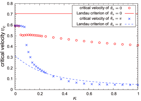
Figure 5: Dependence of the critical velocity $v_{c}$ on the strength of the SO coupling $\kappa$ for $\gamma=0.8$ and $R=0.5$. The red circles and blue crosses indicate the critical velocities for $\theta_{v}=0$ and $\theta_{v}=\pi$, respectively. The red solid line and the blue dashed line indicate the Landau criterion for $\theta_{v}=0$ and $\theta_{v}=\pi$, respectively, in Eq. (15).

Figure 5 shows the $\kappa$ dependence of the critical velocity $v_{c}$. For $\theta_{v}=0$, $v_{c}$ discontinuously decreases at $\kappa\simeq 0.03$, and gradually decreases with increasing in $\kappa$. The discontinuous change is attributed to the $\psi_{1}$-$\psi_{2}$ symmetry breaking in the vortices that are generated by the potential. For $\kappa\gtrsim 0.03$, the vortex cores in the two components are displaced from each other M. Kato , which can be regarded as a pair of half-quantized vortices, whereas the vortices generated for $\kappa\lesssim 0.03$ are the usual topological defects of the global phase in which $\psi_{1}=\psi_{2}$ is preserved. Similarly, for $\theta_{v}=\pi$, the symmetry between the two components is broken for $\kappa\gtrsim 0.08$, causing the sudden change in $v_{L}$. The critical velocity $v_{c}$ is below the Landau critical velocity $v_{L}$ for $\kappa\gtrsim 0.3$, which may be due to the finite size effect of the obstacle potential.

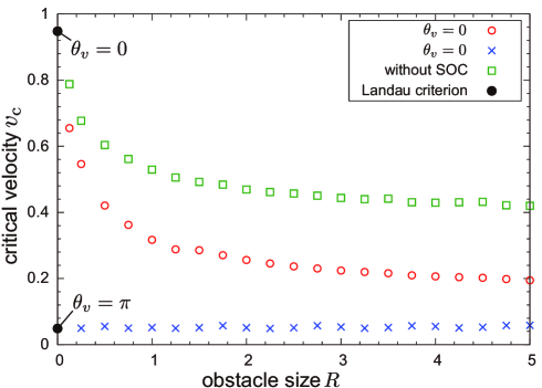
Figure 6: Dependence of critical velocities $v_{c}$ on the obstacle radius $R$ for $\kappa=1$ and $\gamma=0.8$. The red circles and blue crosses indicate the critical velocities for $\theta_{v}=0$ and $\theta_{v}=\pi$, respectively. The green squares indicate the critical velocity without the SOC. The black solid circles indicate the Landau criteria in Eq. (15).

Figure 6 shows the dependence of critical velocity $v_{c}$ on the obstacle radius $R$ for $\theta_{v}=0$ and $\theta_{v}=\pi$. The critical velocity for the system without the SOC is also plotted for comparison. In the limit of small $R$, the critical velocities approach the Landau critical velocity, as expected. The critical velocity with SOC is always smaller than that without the SOC, for the same reason as that for the steep decrease of $v_{c}$ in Fig. 5, i.e., the symmetry breaking between the two components due to the spin dependent force by the SOC tends to decrease the critical velocity. Interestingly, for the case of $\theta_{v}=\pi$, $v_{c}$ is approximately independent of $R$, whereas $v_{c}$ decreases with $R$ for the case of $\theta_{v}=0$.

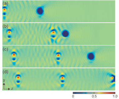
Figure 7: Serial snapshots of the density distributions $|\psi_{1}|^{2}$ of the dynamics in the rest frame for $\kappa=1$ and $\gamma=0.8$. The velocity of the moving obstacle is $(v,\theta_{v})=(0.5,0)$, and the radius is $R=2$. The time interval is 75, and the field of view is $100\times 20$. See the Supplemental Material for movies of the dynamics of of component 1 SM .

Figure 7 shows serial snapshots of the density distribution in the rest frame for $(v,\theta_{v})=(0.5,0)$. The velocity of the vortex pairs released from the moving obstacle potential, $v_{\rm vortex}\simeq 0.05$, is much smaller than that without the SOC M. Kato . In the rest frame, the vortex pairs are created just like a moving obstacle would leave behind them on its trajectory.

V velocity field

Finally, we discuss the velocity field distribution induced by the obstacle potential. The velocity field of the condensate is defined as

$$\bm{v}_{f}(\bm{r})=\frac{1}{2i\rho}\left[\bm{\Psi}^{\dagger}\bm{\nabla}\bm{\Psi}-\bm{\Psi}^{T}\bm{\nabla}\bm{\Psi}^{\ast}\right]-\frac{\kappa}{\rho}\bm{\Psi}^{\dagger}\bm{\sigma}_{\perp}\bm{\Psi},$$ (21)

where $\rho=|\psi_{1}|^{2}+|\psi_{2}|^{2}$. The first term on the right-hand side of Eq. (21) is the usual superfluid velocity, and the second term originates from the SOC. The velocity field satisfies the equation of continuity, $\partial\rho/\partial t+\bm{\nabla}\cdot(\rho\bm{v})=0$. The velocity field far from the obstacle potential vanishes due to the cancellation between the first and second terms of Eq. (21).

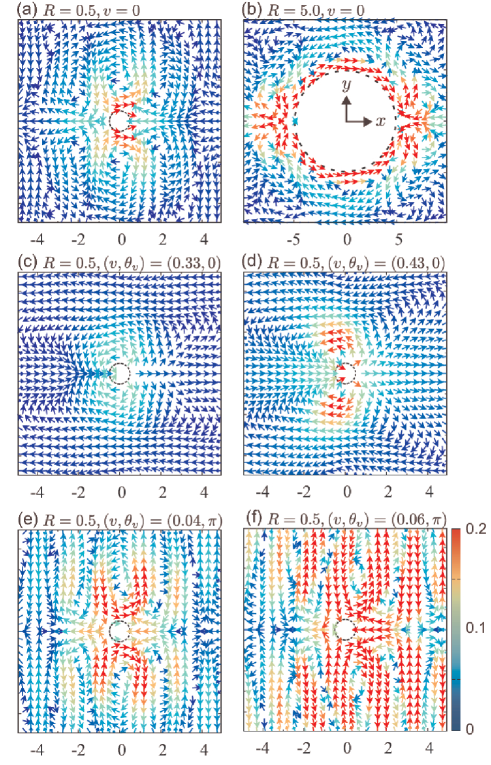
Figure 8: Velocity field distribution induced by an obstacle potential for $\kappa=1$ and $\gamma=0.8$. (a)-(b) Ground states with the obstacle potential at rest. The radii of the circular potential are $R=0.5$ and $5.0$. The velocity of the potential with radius $R=0.5$ is increased as $v(t)=6.0\times 10^{-4}t$ in (c)-(d) and $v(t)=-7.0\times 10^{-5}t$ in (e)-(d). (c)$(v,\theta_{v})=(0.33,0)$ at $t=550$, (d)$(v,\theta_{v})=(0.43,0)$ at $t=717$, (e)$(v,\theta_{v})=(0.04,\pi)$ at $t=600$, and (f)$(v,\theta_{v})=(0.06,\pi)$ at $t=835$. The arrows indicate the direction of the velocity field, and their color indicates the value of $v$. The dashed circle in each panel indicates the obstacle potential.

Figures 8(a) and 8(b) show the velocity field of the ground state with the obstacle potential at rest. Even for the static case, the velocity field exhibits complicated structures containing multiple circulations. A strong rightward flow is observed in the vicinity of the potential, which is explained as follows. The spin-dependent SOC forces on components 1 and 2 are in the $+y$ and $-y$ directions, respectively, which results in the density difference between the two components at the edge of the potential. For the wave function,

$$\bm{\Psi}(\bm{r})=\left(\begin{array}[]{c}u_{1}(\bm{r})e^{i\kappa x}\\ u_{2}(\bm{r})e^{i\kappa x}\end{array}\right),$$ (22)

with real functions $u_{1}$ and $u_{2}$, the velocity field is given by $\bm{v}_{f}=\kappa\rho^{-1}(u_{1}-u_{2})^{2}\bm{e}_{x}$, where $\bm{e}_{x}$ is the unit vector in the $x$ direction. Thus, the density imbalance at the edge of the potential generates the rightward velocity field.

For $\theta_{v}=0$, as the obstacle velocity increases, the circulations in the velocity field vanish and the velocity field becomes similar to that for the system without SOC, as shown in Figs. 8(c) and 8(d). The disappearance of the complicated velocity field is due to the disappearance of the imbalance between $|\psi_{1}|^{2}$ and $|\psi_{2}|^{2}$ by the fast motion of the obstacle.

On the other hand, the velocity field for $\theta_{v}=\pi$ is quite different from the case of $\theta_{v}=0$, as shown in Figs. 8(e) and 8(f). In this case, the flows are mainly along the $y$ direction, and alternately shift upward and downward. This behavior can be understood based on the results of the Bogoliubov analysis in Sec. III.2. Assuming $\gamma=1$, for simplicity, the most unstable wave number is estimated to be $\bm{q}\simeq-2\kappa\bm{e}_{x}$ from Eq. (16), and the eigenvector in Eq. (19) is approximated to be $\bm{\alpha}\propto(1,-1)^{T}$ and $\bm{\beta}\simeq\bm{0}$. Substituting these into Eq. (6), the excited wave function becomes

$$\Psi(\bm{r},t)=\frac{e^{-i\mu t}}{\sqrt{2}}\left[\left(\begin{array}[]{c}1\\ 1\end{array}\right)e^{i\kappa x}+\delta u\left(\begin{array}[]{c}1\\ -1\end{array}\right)e^{-i\kappa x}\right],$$ (23)

where $\delta u$ is an infinitesimal amplitude of the excitation, which is assumed to be real without loss of generality. The velocity field in Eq. (21) is thus obtained as

$$\bm{v}_{f}(\bm{r})=-2\delta u\sin(2\kappa x)\bm{e}_{y},$$ (24)

where $\bm{e}_{y}$ is a unit vector in the $y$ direction. In Fig. 8(f), the wave length of the velocity field is estimated to be $\lambda_{v}\simeq 3$, which agrees well with the wavelength $\pi/\kappa$ in Eq. (24).

VI Conclusions

In conclusion, we have investigated the dynamics of an SO-coupled BEC with a moving obstacle potential. We found that the obstacle potential moving in the plane-wave state exhibits a variety of excitation dynamics. We have shown that the dynamics strongly depend on the direction of the obstacle motion. When the potential moves in the plane-wave direction, half-quantized vortex pairs are released. When the potential moves in the opposite direction, on the other hand, spin waves are dominant. This behavior can be understood from the Bogoliubov spectrum. Although the Landau critical velocity derived from the Bogoliubov spectrum is zero for the other directions, we numerically found that there is an effective critical velocity, below which excitation is negligible and above which the drag force on the obstacle increases steeply. We obtained a diagram of the excitation behavior with respect to the velocity $\bm{v}$ of the potential. We explored the dependence of the effective critical velocity on the strength of the SO coupling $\kappa$ and the obstacle size $R$. We also investigated the velocity field distribution for the system, which exhibits complicated flow patterns depending on the parameters.

- (1) Y.-J. Lin, R. L. Compton, K. Jiménez-García, J. V. Porto, and I. B. Spielman, Nature (London) 462, 628 (2009).
- (2) Y.-J. Lin, K. Jiménez-García, and I. B. Spielman, Nature (London) 471, 83 (2011).
- (3) Y.-J. Lin, R. L. Compton, K. Jiménez-García, W. D. Phillips, J. V. Porto, and I. B. Spielman, Nat. Phys. 7, 531 (2011).
- (4) Y.-J. Lin, R. L. Compton, A. R. Perry, W. D. Phillips, J. V. Porto, and I. B. Spielman, Phys. Rev. Lett. 102, 130401 (2009).
- (5) B. M. Anderson, G. Juzeliūnas, V. M. Galitski, and I. B. Spielman, Phys. Rev. Lett. 108, 235301 (2012).
- (6) Z. Fu, L. Huang, Z. Meng, P. Wang, L. Zhang, S. Zhang, H. Zhai, P. Zhang, and J. Zhang, Nat. Phys. 10, 110 (2014).
- (7) L. Huang, Z. Meng, P. Wang, P. Peng, S.-L. Zhang, L. Chen, D. Li, Q. Zhou, and J. Zhang, Nat. Phys. 12, 540 (2016).
- (8) Z. M. Meng, L. H. Huang, P. Peng, D. H. Li, L. C. Chen, Y. Xu, C. Zhang, P. Wang, and J. Zhang, Rev. Lett. 117, 235304, (2016).
- (9) S. C. Ji, J. Y. Zhang, L. Zhang, Z. D. Du, W. Zheng, Y. J. Deng, H. Zhai, S. Chen, and J. W. Pan, Nat. Phys. 10, 314 (2014).
- (10) Z. Wu, L. Zhang, W. Sun, X.-T. Xu, B.-Z. Wang, S.-C. Ji, Y. Deng, S. Chen, X.-J Liu, J.-W. Pan, Science 354, 83 (2016).
- (11) J. Dalibard, F. Gerbier, Juzeliūnas, and P. Öhberg, Rev. Mod. Phys. 83, 1523 (2011).
- (12) N. Goldman, G. Juzeliūnas, P. Öhberg, and I. B. Spielman, Rep. Prog. Phys. 77, 126401 (2014).
- (13) H. Zhai, Rep. Prog. Phys. 78, 026001 (2015).
- (14) P.-S. He, Y.-H. Zhu, and W.-M. Liu, Phys. Rev. A 89, 053615 (2014).
- (15) R. Liao, O. Fialko, J. Brand, and U. Zülicke, Phys. Rev. A 93, 023625 (2016).
- (16) C. Wang, C. Gao, C.-M. Jian, and H. Zhai, Phys. Rev. Lett. 105, 160403 (2010).
- (17) T.-L. Ho and S. Zhang, Phys. Rev. Lett. 107, 150403 (2011).
- (18) X. F. Zhou, J. Zhou, and C. J. Wu, Phys. Rev. A 84, 063624 (2011).
- (19) S. Sinha, R. Nath, and L. Santos, Phys. Rev. Lett. 107, 270401 (2011).
- (20) H. Hu, B. Ramachandhran, H. Pu, and X.-J. Liu, Phys. Rev. Lett. 108, 010402 (2012).
- (21) T. Kawakami, T. Mizushima, M. Nitta, and K. Machida, Phys. Rev. Lett. 109, 015301 (2012).
- (22) B. Ramachandhran, B. Opanchuk, X.-J. Liu, H. Pu, P. D. Drummond, and H. Hu, Phys. Rev. A 85, 023606 (2012).
- (23) J. Radić, T. A. Sedrakyan, I. B. Spielman, and V. Galitski, Phys. Rev. A 84, 063604 (2011).
- (24) A. L. Fetter, Phys. Rev. A 89, 023629 (2014).
- (25) K. Kasamatsu, Phys. Rev. A 92, 063608 (2015).
- (26) A. Gallemí, M. Guilleumas, R. Mayol, and A. M. Mateo, Phys. Rev. A 93, 033618 (2016).
- (27) Q. Zhu, C. Zhang, and B. Wu, Eur. Phys. Lett. 100, 50003 (2012).
- (28) M. A. Khamehchi,Y. Zhang, C. Hamner,T. Busch, and P. Engels, Phys. Rev. A 90, 063624 (2014).
- (29) S. C. Ji, L. Zhang, X. T. Xu, Z.Wu, Y. Deng, S. Chen, and J. W. Pan, Phys. Rev. Lett. 114, 105301 (2015).
- (30) K. Sun, C. Qu, Y. Xu, Y. Zhang, and C. Zhang, Phys. Rev. A 93, 023615 (2016).
- (31) M. Kato, X.-F. Zhang, and H. Saito, Phys. Rev. A 95, 043605 (2017).
- (32) See Supplemental Material at http:// for movies of the dynamics.