Learning Pixel-Distribution Prior with Wider Convolution for Image Denoising

Abstract

In this work, we explore an innovative strategy for image denoising by using convolutional neural networks (CNN) to learn pixel-distribution from noisy data. By increasing CNN’s width with large reception fields and more channels in each layer, CNNs can reveal the ability of learning pixel-distribution, which is a prior excising in many different types of noise. The key to our approach is a discovery that wider CNNs tends to learn the pixel-distribution features, which provides the probability of that inference-mapping primarily relies on the priors instead of deeper CNNs with more stacked non-linear layers. We evaluate our work: Wide inference Networks (WIN) on additive white Gaussian noise (AWGN) and demonstrate that by learning the pixel-distribution in images, WIN-based network consistently achieves significantly better performance than current state-of-the-art deep CNN-based methods in both quantitative and visual evaluations. Code and models are available at https://github.com/cswin/WIN.

1 Prior: pixel-distribution features

In low-level vision problems, pixel-level features are the most important features. We compare the histograms of different images in various noise levels to investigate the pixel-level features having a certain of consistency. As we can see from Fig. 1 and Fig. 2, the pixel-distribution in noisy images is more similar in higher noise level $\sigma=50$ than lower noise level $\sigma=10$.

WIN inferences noise-free images based on the learned pixel-distribution features. When the noise level is the higher, the pixel-distribution features are more similar. Thus, WIN can learn more pixel-distribution features from noisy images having higher level noise. This is the reason that WIN performs even better in higher-level noise, which can be seen and verified in section 3.

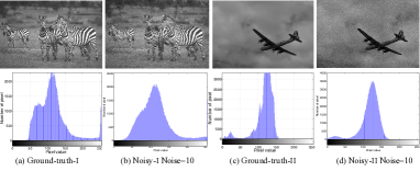
Figure 1: Compare the pixel distributions of histograms of two different images added additive white Gaussian noise (AWGN) with same noise level $\sigma=10$.

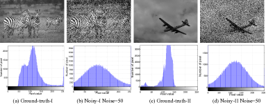
Figure 2: Compare the pixel distributions of histograms of two different images added additive white Gaussian noise (AWGN) with same noise level $\sigma=50$.

2 Wider Convolution Inference Strategy

In Fig. 3, we illustrate the architectures of WIN5, WIN5-R, and WIN5-RB.

2.1 Architectures

Three proposed models have the identical basic structure: $L=5$ layers and $K=128$ filters of size $F=7\times 7$ in most convolution layers, except for the last one with $K=1$ filter of size $F=7\times 7$. The differences among them are whether batch normalization (BN) and an input-to-output skip connection are involved. WIN5-RB has two types of layers with two different colors. (a) Conv+BN+ReLU [19]: for layers 1 to $L-1$, BN is added between Conv and ReLU [19]. (b) Conv+BN: for the last layer, $K=1$ filters of size $F=7\times 7$ is used to reconstruct the $R(y)\approx\displaystyle-n$. In addition, a shortcut skip connecting the input (data layer) with the output (last layer) is added to merge the input data with $R(y)$ as the final recovered image.

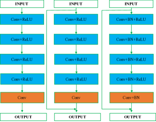
Figure 3: Architectures (a) WIN5 (b) WIN5-R (c) WIN5-RB.

2.2 Having Knowledge Base with Batch-Normal

In this work, we employ Batch Normalization (BN) for extracting pixel-distribution statistic features and reserving training data means and variances in networks for denoising inference instead of using the regularizing effect of improving the generalization of a learned model.

The regularizer-BN can keep the data distribution the same as input: Gaussian distribution. This distribution consistency between input and regularizer ensures more pixel-distribution statistic features can be extracted accurately. The integration of BN [9] into more filters will further preserve the prior information of the training set. Actually, a number of state-of-the-art studies [5, 11, 24] have adopted image priors (e.g. distribution statistic information) to achieve impressive performance.

Can Batch Normalization work without a Skip Connection? In WINs, BN [9] cannot work without the input-to-output skip connection and is always over-fitting. In WIN5-RB’s training, BN keeps the distribution of input data consistent and the skip connection can not only introduce residual learning but also guide the network to extract the certain features in common: pixel-distribution. Without the input data as a comparison, BN could bring negative effects by keeping the each input distribution same, especially, when a task is to output pixel-level feature map. In DnCNN, two BN layers are removed from the first and last layers, by which a certain degree of the BN’s negative effects can be reduced. Meantime DnCNN also highlights network’s generalization ability largely relies on the depth of networks.

In Fig.4, learned priors (means and variances) are preserved in WINs as knowledge base for denoising inference. When WIN has more channels to preserve more data means and variances, various combinations of these feature maps can corporate with residual learning to infer the noise-free images more accurately.

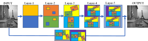
Figure 4: The process of denoising inference by sparse distribution statistics features. Learned priors (means and variances) are preserved in WINs as knowledge base for denoising inference. When WIN has more channels to preserve more data means and variances, various combinations of these feature maps can corporate with residual learning to infer the noise-free images more accurately.

3 Experimental Results

Table 1: The average results of PSNR (dB) / SSIM / Run Time (seconds) of different methods on the BSD200-test [18] (200 images). Note: WIN5-RB-B (blind denoising) is trained on larger number of patches as data augmentation is adapted.This is the reason why WIN5-RB-B (trained on $\sigma=[0-70]$) can outperform WIN5-RB-S (trained on single $\sigma=10,30,50,70$ separately) in some cases.

PSNR (dB) / SSIM
$\sigma$	BM3D [3]	RED-Net [16]	DnCNN [26]	WIN5	WIN5-R	WIN5-RB-S	WIN5-RB-B
10	34.02/0.9182	32.96/0.8963	34.60/0.9283	34.10/0.9205	34.43/0.9243	35.83/0.9494	35.43/0.9461
30	28.57/0.7823	29.05/0.8049	29.13/0.8060	28.93/0.7987	30.94/0.8644	33.62/0.9193	33.27/0.9263
50	26.44/0.7028	26.88/0.7230	26.99/0.7289	28.57/0.7979	29.38/0.8251	31.79/0.8831	32.18/0.9136
70	25.23/0.6522	26.66/0.7108	25.65/0.6709	27.98/0.7875	28.16/0.7784	30.34/0.8362	31.07/0.8962
Run Time(s)
30	1.67	69.25	13.61	15.36	15.78	20.39	15.82
50	2.87	70.34	13.76	16.70	22.72	21.79	13.79
70	2.93	69.99	12.88	16.10	19.28	20.86	13.17

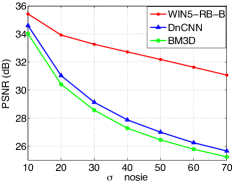
Figure 5: Behavior at different noise levels of average PSNR on BSD200-test. WIN5-RB-B (blind denoising) is trained for $\sigma=[0-70]$ and outperforms BM3D [3] and DnCNN [26] on all noise levels and is significantly more stable even on higher noise levels.

3.1 Quantitative Result

The quantitative result on test set BSD200 is shown on Table 1 including noise levels $\sigma=10,30,50,70$. Moreover, we compare WIN5-RB-B, DnCNN and BM3D behaviors at different noise levels of average PSNR on BSD200-test. As we can see from Fig.5, WIN5-RB-B (blind denoising) trained for $\sigma=[0-70]$ outperforms BM3D [3] and DnCNN [26] on all noise levels and is significantly more stable even on higher noise levels.

In addition, in Fig.5, as the noise level is increasing, the performance gain of WIN5-RB-B is getting larger, while the performance gain of DnCNN comparing to BM3D is not changing much as the noise level is changing. Compared with WINs, DnCNN is composed of even more layers embedded with BN. This observation indicates that the performance gain achieved by WIN5-RB does not mostly come from BN’s regularization effect but the pixel-distribution features learned and relevant priors such as means and variances reserved in WINs. Both Larger kernels and more channels can promote CNNs more likely to learn pixel-distribution features.

3.2 Visual results

For Visual results, We have various images from two different datasets, BSD200-test and Set12, with noise levels $\sigma=10,30,50,70$ applied separately.

One image from BSD200-test with noise level=10

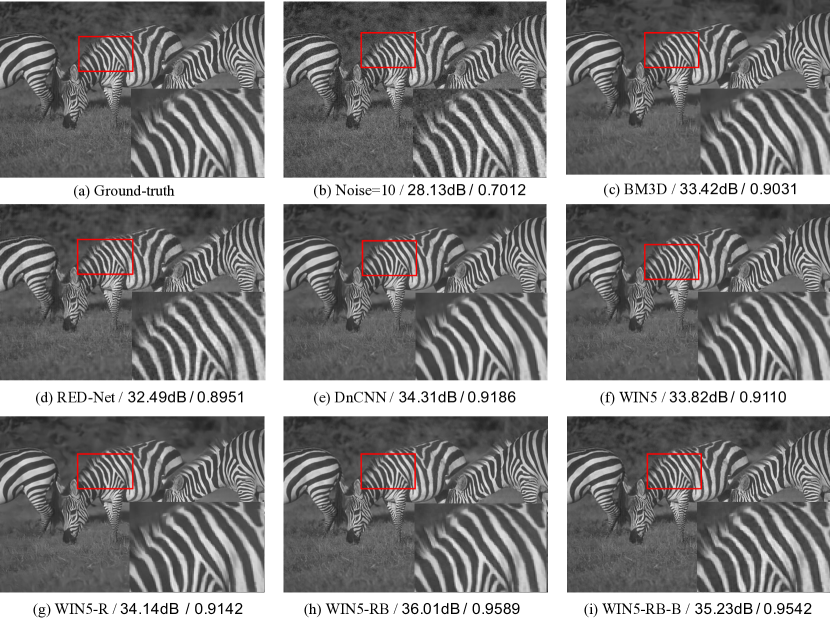
Figure 6: Visual results of one image from BSD200-test with noise level $\sigma=10$ along with PSNR(dB) / SSIM. As we can see, our proposed methods can yield more natural and accurate details in the texture as well as visually pleasant results.

One image from BSD200-test with noise level=30

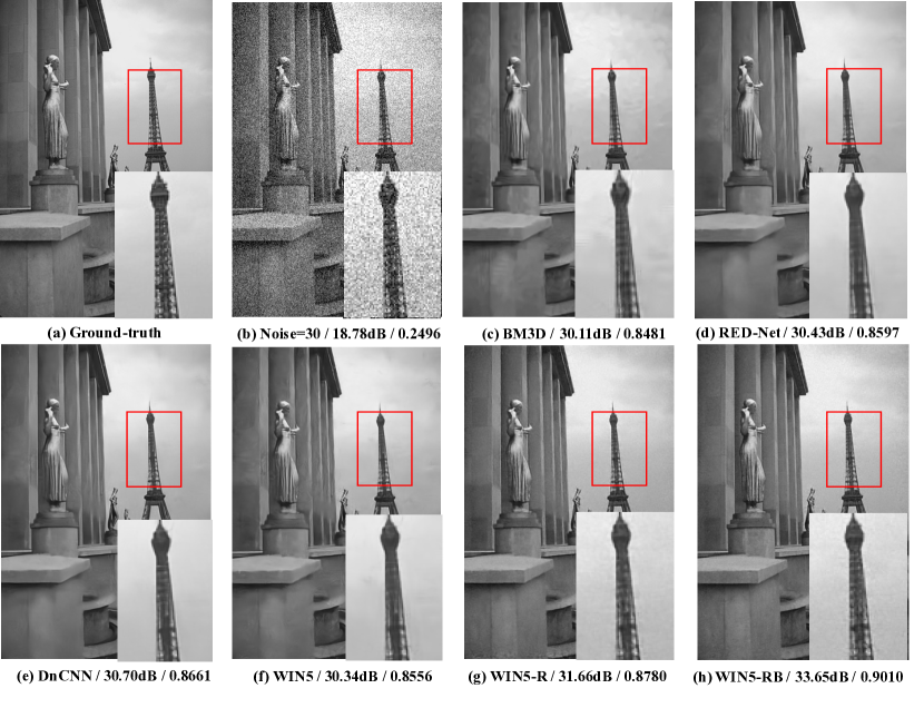
Figure 7: Visual results of one image from BSD200-test with noise level $\sigma=30$ along with PSNR(dB) / SSIM. As we can see, our proposed methods can yield more natural and accurate details in the texture as well as visually pleasant results.

One image from BSD200-test with noise level=50

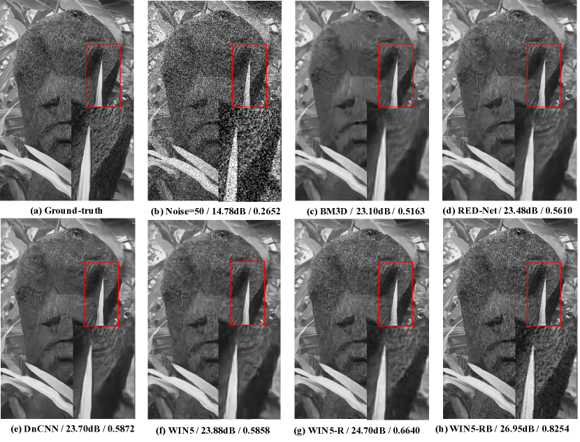
Figure 8: Visual results of one image from BSD200-test with noise level $\sigma=50$ along with PSNR(dB) / SSIM. As we can see, our proposed methods can yield more natural and accurate details in the texture as well as visually pleasant results.

One image from BSD200-test with noise level=70

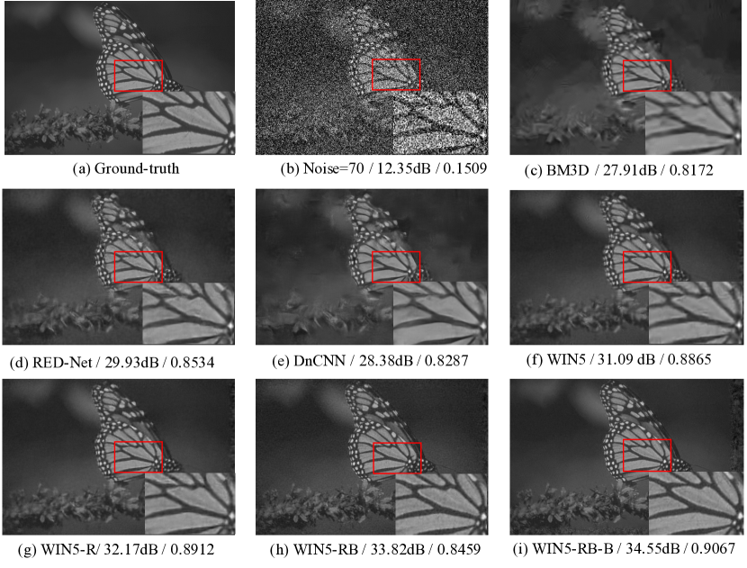
Figure 9: Visual results of one image from BSD200-test with noise level $\sigma=70$ along with PSNR(dB) / SSIM. As we can see, our proposed methods can yield more natural and accurate details in the texture as well as visually pleasant results.

One image from Set12 with noise level=10

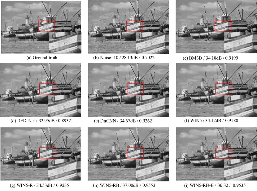
Figure 10: Visual results of one image from Set12 with noise level $\sigma=10$ along with PSNR(dB) / SSIM. As we can see, our proposed methods can yield more natural and accurate details in the texture as well as visually pleasant results.

One image from Set12 with noise level=30

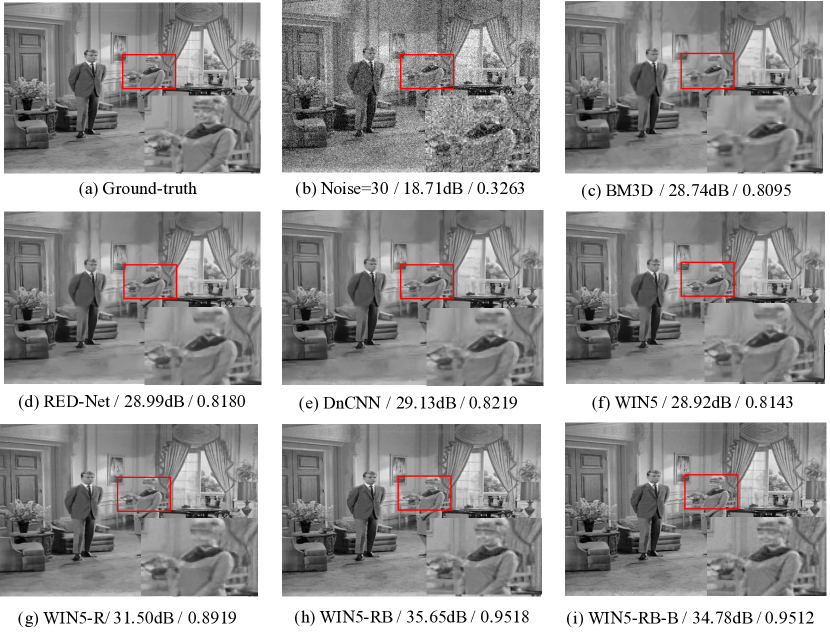
Figure 11: Visual results of one image from Set12 with noise level $\sigma=30$ along with PSNR(dB) / SSIM. As we can see, our proposed methods can yield more natural and accurate details in the texture as well as visually pleasant results.

One image from Set12 with noise level=50

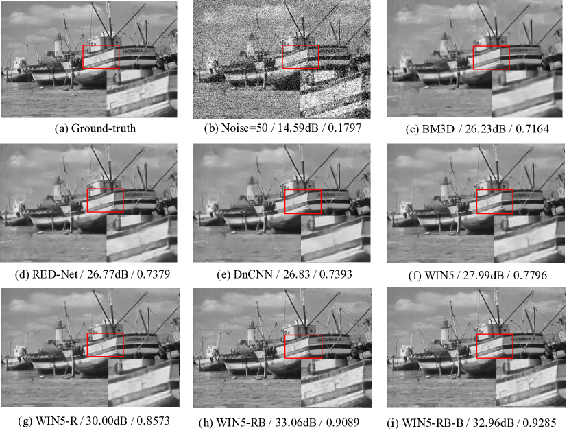
Figure 12: Visual results of one image from Set12 with noise level $\sigma=50$ along with PSNR(dB) / SSIM. As we can see, our proposed methods can yield more natural and accurate details in the texture as well as visually pleasant results.

References

- [1] D. F. Andrews and C. L. Mallows. Scale mixtures of normal distributions. Journal of the Royal Statistical Society. Series B (Methodological), pages 99–102, 1974.
- [2] D. Ciregan, U. Meier, and J. Schmidhuber. Multi-column deep neural networks for image classification. In Computer Vision and Pattern Recognition (CVPR), 2012 IEEE Conference on, pages 3642–3649. IEEE, 2012.
- [3] K. Dabov, A. Foi, V. Katkovnik, and K. Egiazarian. BM3D image denoising with shape-adaptive principal component analysis. In SPARS’09-Signal Processing with Adaptive Sparse Structured Representations, 2009.
- [4] C. Dong, Y. Deng, C. Change Loy, and X. Tang. Compression artifacts reduction by a deep convolutional network. In Proceedings of the IEEE International Conference on Computer Vision, pages 576–584, 2015.
- [5] M. Elad and M. Aharon. Image denoising via sparse and redundant representations over learned dictionaries. IEEE Transactions on Image processing, 15(12):3736–3745, 2006.
- [6] C. Farabet, C. Couprie, L. Najman, and Y. LeCun. Learning hierarchical features for scene labeling. IEEE transactions on pattern analysis and machine intelligence, 35(8):1915–1929, 2013.
- [7] K. He, X. Zhang, S. Ren, and J. Sun. Deep residual learning for image recognition. In Proceedings of the IEEE Conference on Computer Vision and Pattern Recognition, pages 770–778, 2016.
- [8] J. J. Hopfield. Neural networks and physical systems with emergent collective computational abilities. Proceedings of the national academy of sciences, 79(8):2554–2558, 1982.
- [9] S. Ioffe and C. Szegedy. Batch normalization: Accelerating deep network training by reducing internal covariate shift. arXiv preprint arXiv:1502.03167, 2015.
- [10] V. Jain and S. Seung. Natural image denoising with convolutional networks. In Advances in Neural Information Processing Systems, pages 769–776, 2009.
- [11] N. Joshi, C. L. Zitnick, R. Szeliski, and D. J. Kriegman. Image deblurring and denoising using color priors. In Computer Vision and Pattern Recognition, 2009. CVPR 2009. IEEE Conference on, pages 1550–1557. IEEE, 2009.
- [12] D. Kiku, Y. Monno, M. Tanaka, and M. Okutomi. Residual interpolation for color image demosaicking. In 2013 IEEE International Conference on Image Processing, pages 2304–2308. IEEE, 2013.
- [13] J. Kim, J. K. Lee, and K. M. Lee. Accurate image super-resolution using very deep convolutional networks. In The IEEE Conference on Computer Vision and Pattern Recognition (CVPR Oral), June 2016.
- [14] A. Krizhevsky, I. Sutskever, and G. E. Hinton. Imagenet classification with deep convolutional neural networks. In Advances in neural information processing systems, pages 1097–1105, 2012.
- [15] S. Z. Li. Markov random field modeling in image analysis. Springer Science & Business Media, 2009.
- [16] X.-J. Mao, C. Shen, and Y.-B. Yang. Image restoration using convolutional auto-encoders with symmetric skip connections. arXiv preprint arXiv:1606.08921, 2016.
- [17] D. Martin, C. Fowlkes, D. Tal, and J. Malik. A database of human segmented natural images and its application to evaluating segmentation algorithms and measuring ecological statistics. In Computer Vision, 2001. ICCV 2001. Proceedings. Eighth IEEE International Conference on, volume 2, pages 416–423. IEEE, 2001.
- [18] D. Martin, C. Fowlkes, D. Tal, and J. Malik. A database of human segmented natural images and its application to evaluating segmentation algorithms and measuring ecological statistics. In Proc. 8th Int’l Conf. Computer Vision, volume 2, pages 416–423, July 2001.
- [19] V. Nair and G. E. Hinton. Rectified linear units improve restricted boltzmann machines. In Proceedings of the 27th international conference on machine learning (ICML-10), pages 807–814, 2010.
- [20] Y. A. Rozanov. Markov random fields. In Markov Random Fields, pages 55–102. Springer, 1982.
- [21] K. Simonyan and A. Zisserman. Very deep convolutional networks for large-scale image recognition. arXiv preprint arXiv:1409.1556, 2014.
- [22] J. T. Springenberg, A. Dosovitskiy, T. Brox, and M. Riedmiller. Striving for simplicity: The all convolutional net. arXiv preprint arXiv:1412.6806, 2014.
- [23] C. Szegedy, W. Liu, Y. Jia, P. Sermanet, S. Reed, D. Anguelov, D. Erhan, V. Vanhoucke, and A. Rabinovich. Going deeper with convolutions. In Proceedings of the IEEE Conference on Computer Vision and Pattern Recognition, pages 1–9, 2015.
- [24] J. Xu, L. Zhang, W. Zuo, D. Zhang, and X. Feng. Patch group based nonlocal self-similarity prior learning for image denoising. In Proceedings of the IEEE International Conference on Computer Vision, pages 244–252, 2015.
- [25] M. D. Zeiler and R. Fergus. Visualizing and understanding convolutional networks. In European Conference on Computer Vision, pages 818–833. Springer, 2014.
- [26] K. Zhang, W. Zuo, Y. Chen, D. Meng, and L. Zhang. Beyond a gaussian denoiser: Residual learning of deep cnn for image denoising. arXiv preprint arXiv:1608.03981, 2016.