Bunching Effect and Quantum Statistics of Partially Indistinguishable Photons

Abstract

The quantum statistics of particles is determined by both the spins and the indistinguishability of quantum states. Here we studied the quantum statistics of partially distinguishable photons by defining the multi-photon indistinguishability. The photon bunching coefficient was formulated based on the properties of permutation symmetry, and a modified Bose–Einstein statistics was presented with an indistinguishability induced photon bunching effect. Moreover, the statistical transition of the photon state was studied for partially distinguishable photons, and the results shows the that indistinguishability exhibits the same role as that observed in the generation of laser. The results will fill the gap between Bose–Einstein and Poisson statistics for photons, and a formula is presented for the study of multi-photon quantum information processes.

I Introduction

The indistinguishability induced photon bunching effect is the foundation of stimulated emission, multi-photon interference and general statistics QO ; Sun07 . The stimulated emission process is the physical mechanism underlying lasers and superluminescence. With multi-photon interference HOM ; SA ; PanRMP ; Ou , optical quantum information processing has been well developed KLM ; KokRMP ; OBreinSci , and the advantages have been demonstrated in quantum computing via the Shor algorithm Lu07 ; Lanyon07 ; OBrien12 , boson sampling Broome ; Spring ; Tillmann ; Bentivegna15 , and quantum metrology Vittorio11 ; Nagata07 ; SUNEPL ; Xiang11 , which has achieved resolutions that extend beyond classical limits and approach the quantum Heisenberg limit. Additionally, for indistinguishable photons, the general photon number distribution shows Bose–Einstein statistics. However, when photons are partially distinguishable, the fidelity of quantum computing and the resolution of quantum metrology quickly decreases as the photon numbers increase, and in certain cases, the advantages of quantum information processing can be lost. Moreover, the photon number distribution will vary considerably from that of Bose–Einstein statistics. For example, the photon number distribution could show Poisson statistics when the photons are totally distinguishable. However, the properties of photon statistics have not been clarified when photons are partially indistinguishable. Moreover, the bunching effect of partially indistinguishable photons has not been resolved.

In this study, we discuss the role of photon indistinguishability Sun09 in photon statistics. By defining and calculating the indistinguishability ($K_{n}$) of an $n$-photon state, the photon bunching effect is presented and analyzed in detail for partially indistinguishable photons. Both the multi-photon indistinguishability and multi-photon bunching effect show exponential decay with increase in the photon number. Consequently, the photon statistical distribution is modified from the Bose–Einstein statistics ($K_{n}=1$) by considering the partially indistinguishable photon state and approaches the Poisson statistics when the indistinguishability is lost ($K_{n}=0$). Because photon indistinguishability induces notable photon bunching at high photon numbers, the statistical transition of photon state may occur. Such a photon statistical transition can be evaluated by the second-order degree of coherence where the transition point highly depends on the photon indistinguishability.

In general, the statistical distribution of particles can be described as

$$P_{\varepsilon}\propto\frac{1}{\mathrm{e}^{\varepsilon/k_{B}T}-S}\text{,}$$ (1)

where $\varepsilon$ represents the energy, $k_{B}$ represents the Boltzmann constant, and $T$ represents the absolute temperature. The statistical properties of different particles are governed by their spins and the indistinguishability of their quantum states. For indistinguishable Fermions with half-integer spins, $P_{\varepsilon}$ represents Fermi–Dirac statistics with $S=-1$; while for Bosons with integer spins, it shows Bose–Einstein statistics with $S=1$. The main difference between these two distributions is the value of $S$, which describes both the permutation symmetric properties and the indistinguishability induced bunching factor. In typical circumstances, particles are always interacting with other particles or the outer environment, and their quantum coherence may be lost. Thus, particles are in a mixed state and can be partially distinguishable. In this case, the value of $\left|S\right|$ should be between $0$ and $1$. By studying the photon indistinguishability induced bunching effect and photon statistics, we find that $S$ monotonously depends on the value of the indistinguishability. This result will fill the gap in the photon statistics between the indistinguishable case (Bose–Einstein statistics) and the totally distinguishable case (Poisson statistics).

II Multi-photon indistinguishability and bunching effect

Without a loss of generality, we consider a multi-photon state from $N$ separated emitters, which can be described as Sun09

$$\text{{$\rho$}}_{NPhoton}=C_{0}\bigotimes_{k=1}^{N}(\left|\text{vac}\right\rangle\left\langle\text{vac}\right|+c_{k}\rho_{k})\text{,}$$ (2)

where $\rho_{k}$ ($\mathrm{tr}\rho_{k}=1$) describes the quantum state of a single photon. $\left|\text{vac}\right\rangle$ is the vacuum state. $C_{0}$ is a normalization constant and $c_{k}>0$ is a constant determined by the processes of photon generation and collection. For simplicity, we can set all $c_{k}=c$ and $\rho_{k}=\rho$ because all emitters are under the same environment during the photon generation process. A single photon might be in a mixed state, which can be spectrally decomposed as $\rho=\int_{-\infty}^{+\infty}\mathrm{d}\omega f(\omega)\left|\omega\right\rangle\left\langle\omega\right|$ Sun09 , with $\left|\omega\right\rangle=\int_{-\infty}^{+\infty}\mathrm{d}\upsilon g_{\omega}(\upsilon)a^{{\dagger}}(\upsilon)\left|\text{vac}\right\rangle$, where $a^{{\dagger}}$ ($a$) is single photon creation (annihilation) operator. $|g_{\omega}(\upsilon)|^{2}$ ($\int_{-\infty}^{+\infty}|g_{\omega}(\upsilon)|^{2}\mathrm{d}\upsilon=1$) shows the spectrum of the transform limited pulse with a center frequency $\omega$ and a width $\sigma_{g}$, and $f(\omega)$ ($\int_{-\infty}^{+\infty}f(\omega)\mathrm{d}\omega=1$) is the distribution of a center frequency $\omega_{c}$ with a width $\sigma_{f}$.

To discuss the photon indistinguishability induced photon bunching effect and photon statistics, we can define the indistinguishability of $n$ photons as $K_{n}=\mathrm{tr}\rho^{n}$, with $K_{2}\equiv K=\mathrm{tr}\rho^{2}$ Sun09 and $K_{1}=\mathrm{tr}\rho=1$. Thus, when $\sigma_{f}=0$, the single-photon state is a pure state and photons are indistinguishable with $K=1$ and $K_{n}=1$. However, because of interactions between single photons and the outer environment or other photons in the generation process with $\sigma_{f}>0$, photons are partially distinguishable with $0<K_{n(n>1)}<1$. When $\sigma_{f}\gg\sigma_{g}$, the photons are totally distinguishable, with $K_{n}\longrightarrow 0$.

When both $g_{\omega}(\upsilon)=\mathrm{e}^{-(\upsilon-\omega)^{2}/4\sigma_{g}^{2}}/\sqrt[4]{2\mathrm{\pi}\sigma_{g}^{2}}$ and $f(\omega)=\mathrm{e}^{-(\omega-\omega_{c})^{2}/2\sigma_{f}^{2}}/\sqrt{2\mathrm{\pi}\sigma_{f}^{2}}$ are Gaussian functions with widths of $\sigma_{g}$ and $\sigma_{f}$, respectively, we can obtain $K=$ $\sigma_{g}/(\sqrt{\sigma_{g}^{2}+\sigma_{f}^{2}})$ Sun09 . In this case, $K_{n}$ can be analytically derived based on the value of $K$. Since

$$\left\langle\omega_{i}|\omega_{j}\right\rangle=\int\nolimits_{-\infty}^{+\infty}g_{\omega_{i}}^{\ast}(\upsilon)g_{\omega_{j}}(\upsilon)\mathrm{d}\upsilon=\mathrm{e}^{-(\omega_{i}-\omega_{j})^{2}/8\sigma_{g}^{2}}\text{,}$$ (3)

the value of $K_{n}$ can be

$$K_{n} = \int\nolimits_{-\infty}^{+\infty}\mathrm{d}\omega_{1}\mathrm{d}\omega_{2}\cdots\mathrm{d}\omega_{n}f(\omega_{1})f(\omega_{1})\cdots f(\omega_{n})\left\langle\omega_{1}|\omega_{2}\right\rangle\left\langle\omega_{2}|\omega_{3}\right\rangle\cdots\left\langle\omega_{n}|\omega_{1}\right\rangle$$ (4)

$$= \frac{1}{(2\mathrm{\pi}\sigma_{f}^{2})^{n/2}}\int\nolimits_{-\infty}^{+\infty}\mathrm{d}\omega_{1}\mathrm{d}\omega_{2}\cdots\mathrm{d}\omega_{n}\exp[\sum\nolimits_{i=1}^{n}(-\frac{\omega_{i}^{2}}{2\sigma_{f}^{2}})]\times\exp[-\frac{(\omega_{1}-\omega_{2})^{2}+(\omega_{2}-\omega_{3})^{2}+\cdots+(\omega_{n}-\omega_{1})^{2}}{8\sigma_{g}^{2}}]$$

$$= \frac{1}{(\sigma_{f}^{2})^{n/2}\sqrt{\det M_{n\times n}}}\text{,}$$

where the $n\times n$ matrix is

$$M_{n\times n}=\left[\begin{array}[]{cccccc}\frac{1}{2\sigma_{f}^{2}}+\frac{1}{4\sigma_{g}^{2}}&-\frac{1}{8\sigma_{g}^{2}}&0&\cdots&0&-\frac{1}{8\sigma_{g}^{2}}\\ -\frac{1}{8\sigma_{g}^{2}}&\frac{1}{2\sigma_{f}^{2}}+\frac{1}{4\sigma_{g}^{2}}&-\frac{1}{8\sigma_{g}^{2}}&\cdots&0&0\\ 0&-\frac{1}{8\sigma_{g}^{2}}&\frac{1}{2\sigma_{f}^{2}}+\frac{1}{4\sigma_{g}^{2}}&\cdots&0&0\\ \vdots&\vdots&\vdots&\ddots&\vdots&\vdots\\ 0&0&0&\cdots&\frac{1}{2\sigma_{f}^{2}}+\frac{1}{4\sigma_{g}^{2}}&-\frac{1}{8\sigma_{g}^{2}}\\ -\frac{1}{8\sigma_{g}^{2}}&0&0&\cdots&-\frac{1}{8\sigma_{g}^{2}}&\frac{1}{2\sigma_{f}^{2}}+\frac{1}{4\sigma_{g}^{2}}\end{array}\right]\text{.}$$

In the above calculation, we simply set $\omega_{c}=0$ and applied the $n$-dimensional Gaussian integral with

$$\int\nolimits_{-\infty}^{+\infty}\exp(-\frac{1}{2}\sum\nolimits_{i,j=1}^{n}A_{i,j}x_{i}x_{j})\mathrm{d}^{n}x=\sqrt{\frac{(2\mathrm{\pi})^{n}}{\det A}}\text{,}$$

where $A$ is a symmetric positive-definite $n\times n$ matrix GMatrix . The first five terms are listed in Table.1.

Table 1: The values of multi-photon indistinguishability when spectral distributions ($g_{\omega}(\upsilon)$ and $f(\omega)$) of photons are Gaussian.

$n$	$2$	$3$	$4$	$5$	$6$
$K_{n}$	$K$	$\frac{4K^{2}}{3+K^{2}}$	$\frac{2K^{3}}{1+K^{2}}$	$\frac{16K^{4}}{5+10K^{2}+K^{4}}$	$\frac{16K^{5}}{3+10K^{2}+3K^{4}}$

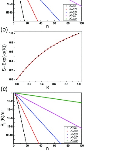
Figure 1: (a) Multi-photon indistinguishability ($K_{n}$) shows exponential decay with the photon number ($n$) for different two-photon indistinguishabilities ($K$). The solid lines are the fittings with Eq.(5). (b) Photon bunching factor ($S=\mathrm{e}^{-\alpha(K)}$) versus the two-photon indistinguishability ($K$). (c) Photon bunching coefficient ($B_{n}$) with the photon number ($n$) for different two-photon indistinguishabilities ($K$). The solid lines are the fittings with Eq.(9). In the calculation, the spectral distributions ($g_{\omega}(\upsilon)$ and $f(\omega)$) of the photons are Gaussian.

Fig. 1(a) shows that the value of $K_{n}$ decays with an increase in the photon numbers. We find that $K_{n}$ ($n\gg 1$) can be well fitted by

$$K_{n}(K)=\mathrm{e}^{-\alpha(K)n}$$ (5)

with a decay rate of $\alpha(K)$. Also, we can find that $K_{n+m}(K)=K_{n}(K)\times K_{m}(K)$. The value of $\mathrm{e}^{-\alpha(K)}$ is also shown in Fig.1 (b). When $K=1$, $\mathrm{e}^{-\alpha(K)}=1$. Additionally, when $K\longrightarrow 0$, $\mathrm{e}^{-\alpha(K)}\longrightarrow 0$.

Because the nonzero $K$ will induce photon bunching, the photon number distribution of $\rho_{NPhoton}$ strongly depends on the value of $K_{n(n>1)}$. Formally, the photon state in Eq.(2) can be re-written as

$$\rho_{NPhoton}=C\sum_{n=0}^{N}\binom{N}{n}B_{n}c^{n}\{n\}\text{,}$$ (6)

where $C$ is a new normalization constant and $\{n\}$ describes the state with the photon number of $n$. $B_{n}$ is an indistinguishability ($K_{n(n>1)}>0$) induced photon bunching coefficient.

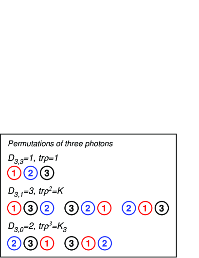
Figure 2: Six ($3!=6$) permutations of three photons for the calculation of three-photon indistinguishability.

Principally, the Bosonic permutation symmetry induces the photon bunching effect Sun07PRA . Here we apply the permutation of $n$ photons to obtain the photon bunching coefficient of an $n$-photon state, which can be described as

$$B_{n}=\sum\limits_{k=2}^{n}D_{n,n-k}K_{k}+1\text{,}$$ (7)

where $D_{n,n-k}=\frac{n!}{(n-k)!}\sum\nolimits_{i=2}^{k}(-1)^{i}/i!$ are rencontres numbers, which show the number of permutations of $n$ photons with $(n-k)$ fixed photons without permutation. Fig.2 illustrates the number of permutations of three photons of $3!=6$, with $D_{3,3}=1$, $D_{3,2}=0$, $D_{3,1}=3$, and $D_{3,0}=2$. Thus, for totally distinguishable states with $K=0$, when $n>1$, $K_{n}=0$ and $B_{n}=1$. For indistinguishable states, $K_{n}=1$, $B_{n}=\sum\nolimits_{k=2}^{n}D_{n,n-k}+1=n!$ shows an $n$-photon bunching result and $\{n\}=\left|n\right\rangle\left\langle n\right|$ is an $n$-photon Fock state. For partially indistinguishable photons, $1<B_{n}<n!$. When $n\gg 1$,

$$\frac{B_{n+1}(K)/(n+1)!}{B_{n}(K)/n!}\rightarrow\frac{K_{n+1}}{K_{n}}=\mathrm{e}^{-\alpha(K)}\text{,}$$ (8)

$B_{n}(K)/n!$ also shows an exponential decay with a photon number with a decay rate of $\alpha(K)$. For the photon state with Gaussian spectral distributions and $n\gg 1$,

$$B_{n}(K)=n!\mathrm{e}^{-\alpha(K)(n-1)}\text{,}$$ (9)

which is shown in Fig.1 (c).

III Photon distribution of partially indistinguishable photons

For totally distinguishable states, $B_{n}=1$, photon bunching does not occur and $\rho_{NPhoton}$ shows a classical state with a binomial distribution. When $N\gg 1$, the binomial distribution converts to Poisson statistics OCQO . For all indistinguishable states with $K_{n}=1$ and $B_{n}=n!$, the photon number distribution of Eq.(2) is

$$\rho_{NPhoton}\simeq(1-Nc)\sum_{n=0}^{N}(Nc)^{n}\left|n\right\rangle\left\langle n\right|=\sum_{n=0}^{N}P_{n}\left|n\right\rangle\left\langle n\right|\text{,}$$ (10)

when $Nc<1$ and $N\gg 1$. It can be described by the Bose–Einstein statistics with

$$P_{n}=\frac{\bar{n}^{n}}{(1+\bar{n})^{n+1}}=P\frac{\mathrm{e}^{-n\varepsilon/k_{B}T}}{\mathrm{e}^{\varepsilon/k_{B}T}-1}\text{,}$$ (11)

where $Nc=\mathrm{e}^{-\varepsilon/k_{B}T}$, $P=\mathrm{e}^{\varepsilon/k_{B}T}+\mathrm{e}^{-\varepsilon/k_{B}T}-2$ and $\bar{n}=Nc/(1-Nc)=1/(\mathrm{e}^{\varepsilon/k_{B}T}-1)$ is the mean photon number.

However, for photons with partial indistinguishability ($0<K_{n}<1$), the photon state should be

$$\rho_{NPhoton} \simeq (1-Nc\mathrm{e}^{-\alpha(K)})\sum_{n=0}^{N}(Nc\mathrm{e}^{-\alpha(K)})^{n}\{n\}$$ (12)

$$= \sum_{n=0}^{N}P_{n}(K)\{n\}\text{.}$$

When $Nc<1$ and $N\gg 1$, a modified Bose–Einstein statistics can be presented as

$$P_{n}(K)=P(K)\frac{\mathrm{e}^{-n[\varepsilon/k_{B}T+\alpha(K)]}}{\mathrm{e}^{\varepsilon/k_{B}T}-S}\text{,}$$ (13)

where $P(K)=\mathrm{e}^{\varepsilon/k_{B}T}+\mathrm{e}^{-\varepsilon/k_{B}T-2\alpha(K)}-2\mathrm{e}^{-\alpha(K)}$, and the mean photon number is $\bar{n}=Nc\mathrm{e}^{-\alpha(K)}/(1-Nc\mathrm{e}^{-\alpha(K)})=1/(\mathrm{e}^{\varepsilon/k_{B}T+\alpha(K)}-1)$. Here, $S=\mathrm{e}^{-\alpha(K)}$ is an indistinguishability induced photon bunching factor. Without changing $N$ and $c$, the statistics is modified from the Bose–Einstein statistics in Eq.(11) via $S$, with $S=1$ for indistinguishable case ($K=1$) and $S=0$ for the totally distinguishable case ($K=0$). The results clearly demonstrates the important role of indistinguishability in photon statistics.

IV Indistinguishability induced photon bunching and statistical transition

Because photons are Bosons, statistical transition can occur when more than one photon occurs in a single mode, which results from the indistinguishability induced photon bunching effect. Here, we apply the second-order degree of coherence ($g^{(2)}(0)$) to evaluate the photon statistical transition. For the single photon state in Eq.(2), $c$ describes the photon emission probability from an emitter and $Nc$ is the number of photons from $N$ emitters without photon bunching. When $Nc\ll 1$, $g^{(2)}(0)=1+K$. However, when $Nc\gg 1$ and $K>0$, more than one photon occurs in the emission mode and the bunching effect from the indistinguishable multi-photon state dominates the quantum statistics, as shown in Eq.(8). This finding demonstrates that photons condensate into an $n$-photon Fock state with $g^{(2)}(0)\rightarrow 1$ when $n\gg 1$. Fig.3 (a) shows the values of $g^{(2)}(0)$ with different values of $K$ and the behavior of photon statistical transitions from $g^{(2)}(0)=1+K$ to $g^{(2)}(0)\rightarrow 1$ with an increase in the photon number $Nc$. For indistinguishable photon state with Bose–Einstein statistics, the transition occurs at $Nc=1$. We found that with lower $K$ values, a higher photon number $Nc$ is required to make the transition. This finding indicates that photon indistinguishability induced photon bunching effect is a key contribution to the transition. Eq.(12) shows that, the transition points should occur approximately at $Nc=1/S$.

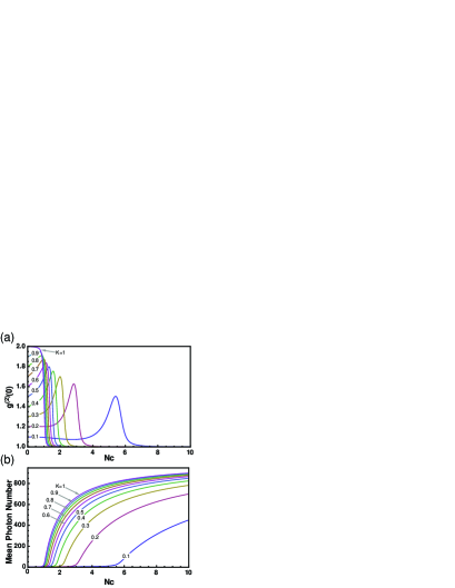
Figure 3: (a) Second-order degree of coherence ($g^{(2)}(0)$) versus $Nc$. (b) Mean photon number versus $Nc$. From left to right, the ten curves in each figure correspond to two-photon indistinguishabilities ($K$) from $1$ to $0.1$. In the calculation, $N=1000$ and the spectral distributions ($g_{\omega}(\upsilon)$ and $f(\omega)$) of the photons are Gaussian.

Such a transition can also be demonstrated by the mean photon numbers ($\bar{n}$) in Fig.3 (b). At a low emission rate ($Nc\ll 1$), spontaneous emission dominates and $\bar{n}$ increases slowly with $Nc$ for different photon indistinguishabilities. However, when $Nc>1/S$, $\bar{n}$ increases quickly with $Nc$ because the bunching effect from indistinguishable photons induces stimulated emission Sun07 and dominates the photon statistics. Higher $K$ values correspond to a higher increase rate. When $Nc\gg 1/S$, $\bar{n}\rightarrow N$, which demonstrates saturation. Fig.3 shows that, although the photon emission in Eq.(2) lacks phase coherence, the photon indistinguishability exhibits the same role as in the generation of laser Abmann .

V Discussion and conclusion

The multi-photon interference is essential for optical quantum information processes. In addition to phase modulation, the photon indistinguishability induced bunching effect is a key parameter in multi-photon interference. Defining and calculating multi-photon indistinguishability ($K_{n}$) are key elements in the analysis of multi-photon interference Sun07 ; Xiang06 ; RaNC and optical quantum information processes. Because multi-photon indistinguishability shows an exponential decay with increases in the photon numbers, such an imperfect indistinguishability is the reason for the exponential decay in the fidelity of multi-photon entangled state and the visibility of multi-photon interference Huang ; Wang16 . Especially in recently developed boson sampling Broome ; Spring ; Tillmann ; Bentivegna15 ; Tillmann15 and quantum metrology Vittorio11 ; Nagata07 ; SUNEPL ; Xiang11 with entangled photon number state, many photons interfere in a same spatial mode. Imperfect interference with partially indistinguishable photons highly decreases the fidelity of quantum computation and the resolution of the quantum metrology. Defining multi-photon indistinguishability provides important insights on these issues.

In conclusion, we have presented the definition of the indistinguishability of multi-photon states. Based on the multi-photon emission model, we discussed the indistinguishability induced bunching effect in photon statistical behavior. The photon statistical distribution can be changed from a classical Poisson distribution to Bose–Einstein statistics when the multi-photon indistinguishability is increased from $0$ to $1$. A modified Bose–Einstein statistics is presented for partially indistinguishable photons with an indistinguishability induced photon bunching factor note . In addition to its influence on photon statistical behavior, multi-photon indistinguishability is a key parameter in multi-photon interference for optical quantum information techniques and in the generation of laser and superluminescence.

References

- (1) M. O. Scully and M. S. Zubairy, Quantum Optics (Cambridge University Press, Cambridge, England, 1997).
- (2) F.-W. Sun, B.-H. Liu, Y.-X. Gong, Y.-F. Huang, Z.Y. Ou, and G.-C. Guo, Phys. Rev. Lett. 99, 043601 (2007).
- (3) C. K. Hong, Z. Y. Ou, and L. Mandel, Phys. Rev. Lett. 59, 2044 (1987).
- (4) Y. H. Shih and C. O. Alley, Phys. Rev. Lett. 61, 2921 (1988).
- (5) J.-W. Pan, Z.-B. Chen, C.-Y. Lu, H. Weinfurter, A. Zeilinger, and M. Żukowski, Rev. Mod. Phys. 84, 777 (2012).
- (6) Z. Y. Ou, Multi-Photon Quantum Interference (Springer, New York, 2007).
- (7) E. Knill, R. Laflamme, and G. Milburn, Nature 409, 46 (2001).
- (8) P. Kok, W. J. Munro, K. Nemoto, T. C. Ralph, J. P. Dowling, and G. J. Milburn, Rev. Mod. Phys. 79, 135 (2007).
- (9) J. L. O’Brien, Science 318, 1567 (2007).
- (10) C.-Y. Lu, D. E. Browne, T. Yang, and J.-W. Pan, Phys. Rev. Lett. 99, 250504 (2007)
- (11) B. P. Lanyon, T. J. Weinhold, N. K. Langford, M. Barbieri, D. F. V. James, A. Gilchrist, and A. G. White, Phys. Rev. Lett. 99, 250505 (2007)
- (12) E. Martín-López, A. Laing, T. Lawson, R. Alvarez, X.-Q. Zhou and J. L. O’Brien, Nat. Photon. 6, 773 (2012).
- (13) M. A. Broome, A. Fedrizzi, S. Rahimi-Keshari, J. Dove, S. Aaronson, T. C. Ralph, A. G. White, Science 339, 794–798 (2013).
- (14) J. B. Spring, B. J. Metcalf, P. C. Humphreys, W. S. Kolthammer, X.-M. Jin, M. Barbieri, A. Datta N. Thomas-Peter, N. K. Langford, D. Kundys, J. C. Gates, B. J. Smith, P. G. R. Smith, I. A. Walmsley, Science 339, 798 (2013).
- (15) M. Tillmann, B. Dakic, R. Heilmann, S. Nolte, A. Szameit, P. Walther, Experimental boson sampling. Nat. Photon. 7, 540 (2013).
- (16) M. Bentivegna, N. Spagnolo, C. Vitelli, F. Flamini, N. Viggianiello, L. Latmiral, P. Mataloni, D. J. Brod, E. F. Galvão, A. Crespi, R. Ramponi, R. Osellame, and F. Sciarrino, Science Adv. 1, e1400255 (2015)
- (17) G. Vittorio, L. Seth, and M. Lorenzo, Nat. Photon. 5, 222 (2011).
- (18) T. Nagata, R. Okamoto, J. L. O’Brien, K. Sasaki, and S. Takeuchi, Science 316, 726 (2007).
- (19) F.-W. Sun, B.-H. Liu, Y.-X. Gong, Y.-F. Huang, Z. Y. Ou, and G.-C. Guo, Europhys. Lett. 82, 24001 (2008).
- (20) G.Y. Xiang, B. L. D. Higgins, W. H. Berry, M. G. Wiseman, and J. Pryde, Nat. Photon. 5, 43 (2011).
- (21) F.-W. Sun and C. W. Wong, Phys. Rev. A 79, 013824 (2009).
- (22) https://en.wikipedia.org/wiki/Gaussian_integral.
- (23) F.-W. Sun, B.-H. Liu, Y.-F. Huang, Y.-S. Zhang, Z. Y. Ou, and G.-C. Guo, Phys. Rev. A 76, 063805 (2007).
- (24) L. Mandel and E. Wolf, Optical Coherence and Quantum Optics (Cambridge University Press, Cambridge, England, 1995). It is not a coherent state from the laser since it is lack of phase coherence.
- (25) M. Aann, F. Veit, M. Bayer, M. van der Poel, and J. M. Hvam, Science 325, 297 (2009).
- (26) G.-Y. Xiang, Y.-F. Huang, F.-W. Sun, P. Zhang, Z.Y. Ou, and G.-C. Guo, Phys. Rev. Lett. 97, 023604 (2006).
- (27) Y.-S. Ra, M. C. Tichy, H. -T. Lim, O. Kwon, F. Mintert, A. Buchleitner, and Y.-H. Kim, Nat. Commun. 4, 2451 (2013).
- (28) Y. F. Huang, B.-H. Liu, L. Peng, Y.-H. Li, L. Li, C.-F. Li, and G.-C. Guo, Nat. Commun. 2, 546 (2011).
- (29) X.-L. Wang, L.-K. Chen, W. Li, H.-L. Huang, C. Liu, C. Chen, Y.-H. Luo, Z.-E. Su, D. Wu, Z.-D. Li, H. Lu, Y. Hu, X. Jiang, C.-Z. Peng, L. Li, N.-L. Liu, Y.-A. Chen, C.-Y. Lu, and J.-W. Pan, Phys. Rev. Lett. 117, 210502 (2016).
- (30) M. Tillmann, S.-H. Tan, S. E. Stoeckl, B. C. Sanders, H. de Guise, R. Heilmann, S. Nolte, A. Szameit, and P. Walther, Phys. Rev. X 5, 041015 (2015).
- (31) Although from Eq.(13), the statistics of partially indistinguishable photons can also be formally written as the Bose–Einstein statistics with extra photon energy () from the permutation of partially indistinguishable photons. However , the extra photon energy is infinite.