Solitary waves and double layers in an adiabatic multi-component space plasma

Abstract

Abstract: The formation and propagation of small amplitude Heavy-ion-acoustic (HIA) solitary waves and double layers in an unmagnetized collisionless multi-component plasma system consisting of superthermal electrons, Boltzmann distributed light ions, and adiabatic positively charged inertial heavy ions are theoretically investigated. The reductive perturbation technique is employed to derive the modified Korteweg-de Vries (mK-dV) and standard Gardner (SG) equations. The solitary wave (SW) solution of mK-dV and SG equations as well as Double Layers (DLs) solution of SG equation is studied for analysis of higher-order nonlinearity. It is found that the plasma system under consideration supports positive and negative potential Gardner solitons but only positive potential mK-dV solitons. In addition, it is shown that, the basic properties of HIA mK-dV and Gardner solitons and DLs (viz. polarity, amplitude, width, and phase speed) are incomparably influenced by the adiabaticity effect of heavy ions and the superthermality effect of electrons. The relevance of the present findings to the system of space plasmas as well as to the system of researchers interest is specified.

Keywords: HIA waves; Effects of Adiabaticity and Superthermality; Gardner solitons and Double Layers.
PACS numbers: 52.35.Fp, 52.35.Mw, 52.35.Tc

I Introduction

The physics of astrophysical plasmas plays the part of most expeditiously growing branches of plasma physics, because such plasmas are omnipresent in space environments Rees1983 ; Miller1987 ; Michel1991 ; Havnes1992 ; Whipple1992 . The ion-acoustic (IA) waves have a crucial role for learning the linear and nonlinear characteristics of various astrophysical plasmas. This type of wave modes are nothing but a low-frequency longitudinal plasma density oscillations which was first anticipated in 1929 by Tonks and Langmuir who defined the phase velocity for isothermal changes and frequencies well below the ion plasma frequency Tonks1929 . In 1933, Revans studied the IA waves experimentally and observed the presence of electrical oscillations within an electrical discharges through gases Revans1933 .

The study of a small population of excess energetic or superthermal electrons within a space plasma system with strong electric fields has proven to be a rich topic with many surprising new phenomena discovered in recent and past years. Astrophysical plasmas are usually hot and collisionless and their characteristics are maintained by the collective wave-particle interactions preferably than individual particle-particle interactions. A number of Satellite or experimental observations have uncovered the presence of excess energetic or superthermal electrons in space and laboratory plasma environments Vasyliunas1968 ; Formisano1973 ; Scudder1981 ; Feldman1982 ; Marsch1982 ; Collier1996 ; Mori2003 ; Papp2015 ; Zeng2015 . The plasma system that contains highly energetic particles with energies greater than thermal energies is studied by using the kappa velocity distribution Vasyliunas1968 ; Baluku2008 ; Baluku2010 . Notably, high energy particles exist due to the effect of external forces acting on the space environment plasmas. Gurevich et al. Gurevich1995 investigated the behaviour of fast or superthermal electrons by deriving the kinetic equation and demonstrated the strong influence of the density profile on the diffusion of fast particles. Lu et al. Lu2011 studied the presence of superthermal electrons in the space plasma and observed the variation of indices of the power law distribution in the magnetosheath. For modeling aforesaid plasmas, kappa velocity distribution is applicable because Boltzmann distribution perhaps inappropriate for explaining the long-range interactions. The generalized three dimensional kappa distribution function Summer1991 is mathematically represented as,

$$F_{k}(v)=\frac{\Gamma(k+1)}{(\pi kw)^{3/2}\Gamma(k-1/2)}(1+\frac{v^{2}}{kw^{2}})^{-(k+1)}$$

Where $F_{k}$ represents the kappa distribution function, $\Gamma$ is the gamma function, $w$ being the most probable speed of the energetic particles, given by $w=[(2k-3/k)^{1/2}(k_{B}T/m)^{1/2}]$, with T shows the characteristic kinetic temperature and $w$ is related to the thermal speed $V_{t}=(k_{B}T/m)^{1/2}$ and, the parameter $k$ symbolizes the spectral index Cattaert2007 which defines the strength of the superthermality. The range of this parameter is $3/2<k<\infty$ Alam2013 . In the limit $k\rightarrow\infty$ Basu2008 ; Baluku2012 , the kappa distribution function lessens to the well-known Boltzmann distribution.

The study of plasmas with impurities (heavy ions or charged dust grains) has been attracted a great deal of interest among the researchers Hines1957 ; Rao1990 ; popel1995a ; popel1996 ; Shukla2002 ; Losseva2009 . Rao et al. Rao1990 considered a dusty plasma system containing dust particles and investigated the linear and nonlinear wave phenomena of dust-acoustic waves. In our present work, the theoretical model is assumed to be composed of inertial heavy ions which is millions to billions times lighter than that of the dust particles. The nonlinear behavior of ion acoustic waves for plasmas containing impurity ions or negatively charged dust particles is examined by Popel and Yu popel1995a since positively charged inertial heavy ions are taken into consideration in our present model. The HIA waves differs from conventional ion acoustic waves in impurity (dust grains) containing plasmas by the following points: i) in Dust-ion-acoustic (DIA) waves the inertia is given by the light ions mass whereas in HIA waves inertia is provided by the heavy ion mass; ii) in HIA waves mobile heavy ions provide the necessary inertia whereas in DIA waves static dust grains participate only in maintaining the equilibrium charge neutrality condition; iii) the frequency of the DIA waves is much greater than that of the HIA waves.

A significant number of attempts have been taken to study the characteristics of plasma system that usually contains ions/heavy-ions or electrons mrHossen2014a ; mrHossen2014b ; mrHossen2014c ; mrHossen2014d ; mrHossen2014e ; BHosen2016a ; BHosen2016b ; Sayed2007 ; Ema2015a ; Ema2015b ; Rahman2007 ; Mamun2008 ; Mahmood2008 ; Fatema2008 ; Hossen2014e ; Hossen2014f ; Hossen2014g ; Hossen2014h . Mahmood et al. Mahmood2008 studied the IA waves in a multi-component plasma system consisting of adiabatically heated ions and observed that the amplitude of electron density humps decreases with the increase of hot ion temperatures. A degenerate quantum plasma system is thought out by Hossen et al. Hossen2014e ; Hossen2014f ; Hossen2014g ; Hossen2014h who studied the roles of heavy ions on HIA waves. In former time, Hines considered a multi-ion plasma system in the ionosphere and studied the effect of heavy ions on the propagation of radio waves Hines1957 . Mamun et al. Mamun2008 observed the combined effects of adiabatic electrons and negatively charged static dust that how they modify the basic properties of the DIA K-dV solitons by studying a dusty plasma system. A lot of investigations have also been made to study the energetic particles by a number of plasma scientists. Barbosa et al. Barbosa1980 considered a model for the generation of banded electrostatic emissions by superthermal electrons employing a power law form which can apply to Jupiter’s magnetosphere and concentrated on instability in the upper hybrid and lower harmonic bands. Basu Basu2008 addressed a plasma system with kappa distributed plasma particles in order to explain the distinguishing features of the kappa distributions. Using kinetic theoretical approach, the basic features of electron acoustic waves in a plasma system whose electrons are two-kappa distributed are studied by Baluku et al. Baluku2011 . Mehran Mehran2012 considered an unmagnetized plasma including cool ions and hot ions with kappa distributed electrons and investigated the basic properties of IA waves where the suprathermality effects play vital roles. Later, Baluku et al. Baluku2012 studied the features of IA solitons in a plasma system with both electron components are kappa-distributed found in Saturn’s magnetosphere. Eslami et al. Eslami2011 thought out an unmagnetized plasma system containing warm adiabatic ions, superthermal electrons, and thermal positrons and found the effects of the spectral index $k$ on the IA waves.

Therefore, the effects of superthermal electrons and adiabatic heavy ions on the propagaton of HIA waves in EI plasmas have been investigated. We have studied the basic properties of small amplitude HIA waves by using the reductive perturbation method in concerning plasma system. To the best of our knowledge no theoretical investigations have been made to investigate the HIA solitary waves in EI plasmas comprising of superthermal electrons, Boltzmann distributed light ions, and adiabatic positively charged inertial heavy ions. Thus, our present attempt is to investigate the contribution of superthermality of electrons and adiabaticity of heavy ions on the nonlinear propagation of HIA waves.

The remainder of this paper is arranged as follows: The basic governing equations are provided in sect. II. The mK-dV and SG equations are derived in sects. III and IV, and their solitary wave solutions are analyzed in sect. V, respectively. DL solution of SG equation is analyzed in sect. VI. Finally, a brief results and discussion is presented in sect. VII.

II The basic governing equations

The propagation of HIA waves in an unmagnetized, collisionless plasma system containing superthermal electrons, Boltzmann distributed light ions, and adiabatic positively charged inertial heavy ions has been considered. At equilibrium, we have $Z_{i}n_{i0}+Z_{h}n_{h0}=n_{e0}$, where $n_{i0},n_{h0}$, and $n_{e0}$ are the unperturbed light ion, heavy ion, and electron number density, $Z_{i}$ is the ion number state, and $Z_{h}$ is the number of light ions residing on the heavy ion’s surface.

The dynamics of HIA waves in such an adiabatic plasma system is governed by the following equations:

$$\hskip 28.45274pt\frac{\partial n_{h}}{\partial t}+\frac{\partial}{\partial x}(n_{h}u_{h})=0,$$ (1)

$$\hskip 28.45274pt\frac{\partial u_{h}}{\partial t}+u_{h}\frac{\partial u_{h}}{\partial x}+\frac{\partial\psi}{\partial x}+\frac{\sigma}{n_{h}}\frac{\partial p_{h}}{\partial x}=0,$$ (2)

$$\hskip 28.45274pt\frac{\partial p_{h}}{\partial t}+u_{h}\frac{\partial p_{h}}{\partial x}+\gamma_{h}p_{h}\frac{\partial u_{h}}{\partial x}=0,$$ (3)

$$\hskip 28.45274pt\frac{\partial^{2}\psi}{\partial x^{2}}=-n_{h}+\beta n_{e}-\alpha n_{i},$$ (4)

where the number density of the plasma species $(n_{j})$ (j= h, i, e; h for heavy ion, i for light ion, e for electron), heavy ion number density $(n_{h})$, heavy ion thermal pressure $(p_{h})$, heavy ion fluid speed $(u_{h})$, and electrostatic potential $(\psi)$ are normalized by ion/electron equilibrium number density $n_{j0}$, heavy ion number density at equilibrium multiplied by number of electrons residing on the heavy ion $Z_{h}n_{h0}$, $Z_{h}n_{h0}T_{h}$, effective heavy ion acoustic velocity $C_{h}=\sqrt{T_{e}/m_{h}}$, and the quantity $T_{e}/e$. The space and time variables are normalized by the Debye radius $\lambda_{D}=\sqrt{T_{e}/4\pi Z_{h}n_{h0}e^{2}}$ and the reciprocal heavy ion plasma frequency ${\omega_{h}}^{-1}=(4\pi e^{2}Z_{h}n_{h0}/m_{h})^{1/2}$, e is the magnitude of the charge of electron. Furthermore, $\sigma=(T_{h}/T_{e})$, $\alpha=(Z_{i}n_{i0}/Z_{h}n_{h0})$, and $\beta=(n_{e0}/Z_{h}n_{h0})$.

It is noted here that for an isothermal process $\gamma_{s}=1$ and $p_{s}=n_{s}$ with constant $T_{s}$ $(i.e.,T_{s}=T_{s0})$, where $s$ is the concerning plasma species taken as adiabatic in the corresponding model. For adiabatic ion fluid, $\gamma_{s}=3$ is taken into accountMamun2008 .

For Modelling the effects of superthermal electrons we have considered the following kappa distribution

$$\hskip 14.22636ptn_{e}=n_{e0}[1-\frac{e\psi}{{T_{e}}(k-\frac{3}{2})}]exp(-k+\frac{1}{2}),\$$ (5)

here, the superthermal parameter k stands for kappa distribution. It is notable that the range of k is $1.6\sim 2.2$ Eslami2012 ; Alam2014 .

The well-known Maxwell-Boltzmann distribution has been considered for light ions. In this case, we have obtained the following Maxwellian light ion number density.

$$\hskip 14.22636ptn_{i}=n_{i0}exp(\frac{-e\psi}{T_{i}}),$$ (6)

where, $n_{e}$ $(n_{i})$ is the number density of the perturbed electrons (light ions) and $T_{e}$ $(T_{i})$ is the temperature of electrons (light ions), respectively.

III Derivation of the modified K-dV equation

We have examined the electrostatic perturbations propagating in an unmagnetized collisionless plasma system due to the effect of dispersion. By considering higher order term, we have derived mK-dV equation employing reductive perturbation method using Eqs. (1) - (4), a set of stretched coordinates Maxon1974 ; Shah2015a ; Shah2015b ; Rahman2014 has introduced for the mK-dV equation as

$$\hskip 14.22636pt\eta={\epsilon}(x-V_{p}t),$$ (7)

$$\hskip 14.22636ptT={\epsilon}^{3}t$$ (8)

where $V_{p}$ is the wave phase speed ($\omega/k$ with $\omega$ being angular frequency and $k$ being the wave number of the perturbation mode), and $\epsilon$ is a smallness parameter measuring the weakness of the dispersion ($0<\epsilon<1$). Now, we have expanded $n_{j}$, $u_{h}$, $p_{h}$ and $\psi$ in power series of $\epsilon$ in the following way,

$$\hskip 14.22636ptn_{j}=1+\epsilon n_{j}^{(1)}+\epsilon^{2}n_{j}^{(2)}+\epsilon^{3}n_{j}^{(3)}+\cdot\cdot\cdot,$$ (9)

$$\hskip 14.22636ptu_{h}=0+\epsilon u_{h}^{(1)}+\epsilon^{2}u_{h}^{(2)}+\epsilon^{3}u_{h}^{(3)}+\cdot\cdot\cdot,$$ (10)

$$\hskip 14.22636ptp_{h}=1+\epsilon p_{h}^{(1)}+\epsilon^{2}p_{h}^{(2)}+\epsilon^{3}p_{h}^{(3)}+\cdot\cdot\cdot,$$ (11)

$$\hskip 14.22636pt\psi=0+\epsilon\psi^{(1)}+\epsilon^{2}\psi^{(2)}+\epsilon^{3}\psi^{(3)}+\cdot\cdot\cdot.$$ (12)

By substituting the values of $\eta$, $T$, and expansions (9)-(12) into (1) - (4) and taking the coefficient of $\epsilon^{2}$ from equations (1)-(3), and $\epsilon$ from (4), we have $n_{j}^{(1)}=u_{j}^{(1)}/V_{p}$, $u_{h}^{(1)}=V_{p}\psi^{(1)}/V_{p}^{2}-\gamma\sigma$, $n_{h}^{(1)}=\psi^{(1)}/V_{p}^{2}-\gamma\sigma$, $p_{h}^{(1)}=\gamma\psi^{(1)}/(V_{p}^{2}-\gamma\sigma)$, and

$$V_{p}=\sqrt{\frac{2k-3}{\alpha\sigma_{i}(2k-3)+\beta(2k-1)}+\gamma\sigma}$$

where $\sigma_{i}=T_{e}/T_{i}$ and $V_{p}$ represents the dispersion relation for the HIA type electrostatic waves in an EI plasma under consideration.

Taking the coefficient of $\epsilon^{3}$, we have obtained a set of equations, which, after using the values of $n_{h}^{(1)}$, $u_{h}^{(1)}$, and $p_{h}^{(1)}$, can be simplified as

$$n_{h}^{(2)}=\frac{3V_{p}^{2}-2\sigma\gamma+\sigma\gamma^{2}}{2(V_{p}^{2}-\sigma\gamma)^{3}}(\psi^{(1)})^{2}+\frac{\psi^{(2)}}{V_{p}^{2}-\sigma\gamma},$$ (13)

$$u_{h}^{(2)}=\frac{V_{p}^{3}+V_{p}\sigma\gamma^{2}}{2(V_{p}^{2}-\sigma\gamma)^{3}}(\psi^{(1)})^{2}+\frac{V_{p}\psi^{(2)}}{V_{p}^{2}-\sigma\gamma},$$ (14)

$$p_{h}^{(2)}=\frac{\gamma(\psi^{(1)})^{2}}{2(V_{p}^{2}-\sigma\gamma)^{2}}+\frac{\gamma u_{h}^{(2)}}{V_{p}}+\frac{\gamma^{2}(\psi^{(1)})^{2}}{2(V_{p}^{2}-\sigma\gamma)^{2}},$$ (15)

$${\rho^{(2)}}=\frac{1}{2}A(\psi^{(1)})^{2},$$ (16)

where

$$A=[\frac{3V_{p}^{2}-2\sigma\gamma+\sigma\gamma^{2}}{(V_{p}^{2}-\sigma\gamma)^{3}}+\beta\frac{1-4k^{2}}{(2k-3)^{2}}+\alpha{\sigma_{i}}^{2}]$$ (17)

To the next higher order of $\epsilon$, we obtain a set of equations

$$\frac{\partial n_{h}^{(1)}}{\partial T}-V_{p}\frac{\partial n_{h}^{(3)}}{\partial\eta}+\frac{\partial u_{h}^{(3)}}{\partial\eta}+\frac{\partial}{\partial\eta}[u_{h}^{(2)}n_{h}^{(1)}$$

$$\hskip 99.58464pt+n_{h}^{(2)}u_{h}^{(1)}]=0,$$ (18)

$$\frac{\partial u_{h}^{(1)}}{\partial T}-V_{p}\frac{\partial u_{h}^{(3)}}{\partial\eta}+\frac{\partial}{\partial\eta}[u_{h}^{(1)}u_{h}^{(2)}]+\frac{\partial\psi^{(3)}}{\partial\eta}$$

$$\hskip 51.21495pt+\sigma\frac{\partial p_{h}^{(3)}}{\partial\eta}-\sigma n_{h}^{(1)}\frac{\partial p_{h}^{(2)}}{\partial\eta}=0,$$ (19)

$$\frac{\partial p_{h}^{(1)}}{\partial T}-V_{p}\frac{\partial p_{h}^{(3)}}{\partial\eta}+u_{h}^{(1)}\frac{\partial p_{h}^{(2)}}{\partial\eta}+u_{h}^{(2)}\frac{\partial p_{h}^{(1)}}{\partial\eta}$$

$$\hskip 5.69054pt+\gamma\frac{\partial u_{h}^{(3)}}{\partial\eta}+\gamma p_{h}^{(1)}\frac{\partial u_{h}^{(2)}}{\partial\eta}+\gamma p_{h}^{(2)}\frac{\partial u_{h}^{(1)}}{\partial\eta}=0,$$ (20)

$$\frac{\partial^{2}\psi^{(1)}}{\partial\eta^{2}}=-n_{h}^{(3)}-\beta\left[\frac{(2k+3)(1-4k^{2})}{6(2k-3)^{3}}(\psi^{(1)})^{3}\right.$$

$$\hskip 28.45274pt\left.+\frac{(1-4k^{2})}{(2k-3)^{2}}\psi^{(1)}\psi^{(2)}+\frac{(1-2k)}{2k-3}\psi^{(3)}\right]$$

$$\hskip 22.76219pt+\alpha\left[{\sigma_{i}}{\psi^{(3)}}-{\sigma_{i}}^{2}\psi^{(1)}\psi^{(2)}+\frac{1}{6}{\sigma_{i}}^{3}({\psi^{(1)}})^{3}\right]\$$ (21)

Now combining Eqs. (18) - (21) and using the values of $n_{h}^{(2)}$, $u_{h}^{(2)}$, $p_{h}^{(2)}$ and $\rho^{(2)}$, we obtain an equation of the form

$$\frac{\partial\psi^{(1)}}{\partial T}+\alpha_{1}\alpha_{2}({\psi^{(1)}})^{2}\frac{\partial\psi^{(1)}}{\partial\eta}+\alpha_{2}\frac{\partial^{3}\psi^{(1)}}{\partial\eta^{3}}=0,$$ (22)

where the value $\alpha_{1}$ and $\alpha_{2}$ is given by

$$\alpha_{1}=\frac{15V_{p}^{4}+9V_{p}^{2}\sigma\gamma^{2}-17V_{p}^{2}\sigma\gamma-5\sigma^{2}\gamma^{3}}{2(V_{p}^{2}-\sigma\gamma)^{5}}$$

$$\hskip 14.22636pt+\frac{3\sigma^{2}\gamma^{4}+6\sigma^{2}\gamma^{2}}{2(V_{p}^{2}-\sigma\gamma)^{5}}+\frac{\sigma\gamma^{2}+\sigma\gamma^{3}}{2(V_{p}^{2}-\sigma\gamma)^{4}}$$

$$\hskip 14.22636pt+\frac{\beta(2k+3)(1-4k^{2})}{2(2k-3)^{3}}-\frac{\alpha}{2}\sigma_{i}^{3},$$ (23)

$$\alpha_{2}=\frac{{(V_{p}^{2}-\sigma\gamma)}^{2}}{2V_{p}},$$ (24)

In order to trace the influence of different plasma parameters on the propagation of HIA waves in our considered plasma system, we have derived the mK-dV equation (22). The stationary solitary wave solution of standard mK-dV equation is obtained by considering a frame $\xi=\eta-u_{0}T$ (moving with speed $u_{0}$) and the solution is,

$$\hskip 5.69054pt{\rm\psi^{(1)}}=\rm\psi_{m}{\rm sech}(\frac{\xi}{\delta}),$$ (25)

where the amplitude, $\psi_{m}=\sqrt{6u_{0}/\alpha_{1}\alpha_{2}}$, and the width, $\delta=\psi_{m}\sqrt{\gamma_{1}},{\gamma_{1}}=\alpha_{1}/6$ and $u_{0}$ is the plasma species speed at equilibrium. The amplitude and width variation of mK-dV solitons are nearly valid around critical value $(k=k_{c})$. The mK-dV equation has a SW solution around $k=k_{c}$, but not any DLs solution. Therefore, we proceed into next higher-order nonlinear equation known as SG equation, because the SG equation supports both SWs and DLs just at the critical value obtained from $A=0$.

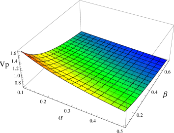
Figure 1: The variation of phase speed $V_{p}$ with $\alpha$ and $\beta$. The other parameters are fixed at $k=2.3$, $\sigma=0.03$, $\sigma_{i}=1.4$, and $U_{0}=0.01$.

IV Derivation of SG Equation

It is obvious from Eq. (16) that $A=0$ since $\psi^{(1)}\neq 0$. We also found that $A=0$ around its critical value $k=k_{c}$. We then assume $A=A_{0}$ when $k\neq k_{c}$ and $k$ is close to $k_{c}$ that $\mid k=k_{c}\mid=\epsilon$ and we can represent $A=0$ as

$$\hskip 5.69054ptA_{0}\simeq s\left(\frac{\partial A}{\partial k}\right)_{k=k_{c}}|k-k_{c}|=sC_{1}\epsilon,$$ (26)

where $|k-k_{c}|$ is a small and dimensionless parameter, and can be taken as the expansion parameter $\epsilon$, i.e. $|k-k_{c}|\simeq\epsilon$, and $s=1$ for $k<k_{c}$ and $s=-1$ for $k>k_{c}$. $C_{1}$ is a constant depending on the superthermality parameter $k$, and is given by

$$\hskip 8.53581ptC_{1}=\frac{1-4k^{2}}{(2k-3)^{2}}.$$ (27)

So, $\rho^{(2)}$ can be expressed as

$$\hskip 8.53581pt\epsilon^{2}\rho^{(2)}\simeq-\epsilon^{3}\frac{1}{2}C_{1}s({\psi^{(1)}})^{2},$$ (28)

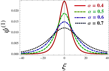
Figure 2: The variation of the positive potential mK-dV solitons with $\alpha$. The other parameters are fixed at $k=2.3$, $\sigma=0.03$, $\beta=0.4$, $\sigma_{i}=1.4$, and $U_{0}=0.01$.

which, therefore, must be included in the third order Poisson’s equation. To the next higher order in $\epsilon^{3}$, we obtain the following equation

$$\frac{\partial^{2}\psi^{(1)}}{\partial\eta^{2}}+\frac{1}{2}sC_{1}({\psi^{(1)}})^{2}-n_{h}^{(3)}-\beta\left[\frac{(2k+3)(1-4k^{2})}{(2k-3)^{3}}\right.$$

$$\left.({\psi^{(1)}})^{3}+\frac{(1-4k^{2})}{(2k-3)^{3}}\psi^{(1)}\psi^{(2)}+\frac{(1-2k)}{(2k-3)}\psi^{(3)}\right]$$

$$-\alpha\left[\sigma_{i}\psi^{(3)}-\sigma_{i}^{2}\psi^{(1)}\psi^{(2)}+\frac{1}{6}\sigma_{i}^{3}({\psi^{(1)}})^{3}\right]=0.$$ (29)

After simplification, we can write from Eq. (29)

$$\frac{\partial\psi^{(1)}}{\partial T}+sC_{1}\alpha_{2}\psi^{(1)}\frac{\partial\psi^{(1)}}{\partial\eta}+\alpha_{1}\alpha_{2}({\psi^{(1)}})^{2}\frac{\partial\psi^{(1)}}{\partial\eta}$$

$$\hskip 108.12047pt+\alpha_{2}\frac{\partial^{3}\psi^{(1)}}{\partial\eta^{3}}=0.$$ (30)

Equation (30) is known as SG equation. It is also called mixed mK-dV equation Lee2009 . It supports both the SWs and DLs solutions since it contains both $\psi$-term of korteweg-de-Vries (K-dV) and $\psi^{2}$-term of mK-dV equation. The Gardner equation derived here is valid for $k\simeq k_{c}$. Figures 5-7 show the variation of the amplitude of positive and negative GSs with $k$ and number density ratio $\beta$ respectively.

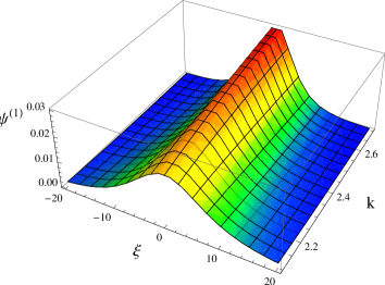
Figure 3: The variation of the positive potential mK-dV solitons for different values of spectral index $k$. The other parameters are fixed at $\alpha=0.4$, $\sigma=0.03$, $\beta=0.4$, $\sigma_{i}=1.4$, and $U_{0}=0.01$.

V SW Solution of SG Equation

The SW solution of SG equation is given by the following equation Alam2014 :

$$\hskip 5.69054pt\psi^{(1)}=\left[\frac{1}{\psi_{m2}}-\left(\frac{1}{\psi_{m2}}-\frac{1}{\psi_{m1}}\right)\cosh^{2}\left(\frac{\xi}{\Delta}\right)\right]^{-1},$$ (31)

where

$$\hskip 5.69054pt\psi_{m1,2}=\psi_{m}\left[1\mp\sqrt{1+\frac{U_{0}}{V_{0}}}\right],$$ (32)

$$\hskip 5.69054ptU_{0}=\frac{sC_{1}B}{3}\psi_{m1,2}+\frac{\alpha_{1}B}{6}\psi_{m1,2}^{2},$$ (33)

$$\hskip 5.69054ptV_{0}=\frac{C_{1}^{2}s^{2}B}{6\alpha_{1}},$$ (34)

$$\hskip 5.69054pt\psi_{m}=\frac{-C_{1}s}{\alpha_{1}},$$ (35)

$$\hskip 5.69054pt\Delta=\frac{2}{\sqrt{-\gamma\psi_{m1}\psi_{m2}}}.$$ (36)

$$\hskip 5.69054pt\gamma=\frac{\alpha_{1}}{6}.$$ (37)

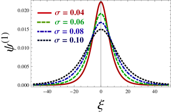
Figure 4: The variation of the positive potential mK-dV solitons with $\sigma$. The other parameters are fixed at $k=2.3$, $\alpha=0.4$, $\sigma_{i}=1.4$, $\beta=0.4$, and $U_{0}=0.01$.

VI DL Solution of SG Equation

The DL solution of Eq. (30) is given by

$$\hskip 5.69054pt\psi^{(1)}=\frac{\psi_{m}}{2}\left[1+\tanh\left(\frac{\xi}{\Delta}\right)\right],$$ (38)

with

$$\hskip 5.69054ptU_{0}=-\frac{s^{2}B}{6\alpha_{1}},$$ (39)

$$\hskip 5.69054pt\psi_{m}=\frac{6U_{0}}{sB},$$ (40)

$$\hskip 5.69054pt\Delta=\frac{2}{\psi_{m}\sqrt{-\gamma}},$$ (41)

where $\gamma=\alpha_{1}/6$ and $\psi_{m}$ ($\Delta$) is the DL height (thickness). This clearly indicates that Eq. (38) represents a DL solution if and only if $\gamma<0$, i.e., $\alpha_{1}<0$. When $\alpha_{1}B=0$, then, in this case, we can find the value of the parameter $k$ as the critical one ($k=k_{d}\approx 1.29$) for a set of plasma parameters viz. $\sigma_{i}=1.6$, $\beta=0.7$, and $U_{0}=0.01$. For $k_{d}<1.29$, $\alpha_{1}<0$, DL does not form. Therefore, positive potential DLs exist for $k_{d}>1.29$ and $s=1$ in our considered plasma system. Fig. 8 indicates the variation of the amplitude of positive DLs with $\alpha$.

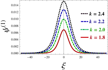
Figure 5: The variation of the positive potential GS solitons with $k$. The other parameters are fixed at $\alpha=0.4$, $\sigma_{i}=1.4$, $\beta=0.4$, and $U_{0}=0.01$.

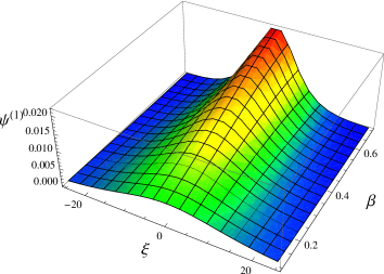
Figure 6: The variation of the positive potential GS solitons for different values of $\beta$. The other parameters are fixed at $k=2.3$, $\alpha=0.4$, $\sigma_{i}=1.4$, and $U_{0}=0.01$.

VII Results and Discussion

In our present investigation, the small amplitude HIA solitary waves rely on plasma parameters, namely the ion to heavy ion number density ratio $\alpha$, the electron to heavy ion number density $\beta$ and th temperature ratio $\sigma$. From the expression of $V_{p}$ it is clear that the phase speed decreases by the plasma parameters $\alpha$ and $\beta$. Figures 1-8 show how the basic features of the HIA waves are significantly varied in the presence of superthermal electrons, Boltzmann distributed light ions, and adiabatic positively charged inertial heavy ions. The phase speed $V_{p}$ has been changed moderately due to the effects of $\alpha$ and $\beta$ which are shown in Fig. 1. The amplitude of the HIA solitary waves decreases with the increasing of $\alpha$ and $\beta$ due to the increasing of inertia (see Figs. 2 and 4). The spectral index $k$ has a vital role on the forming of solitary structures. For small values of $k$ the superthermal electrons in the tail of velocity distribution function increases and, vice versa. In case of mK-dV solitons only positive potentials have been found which is shown in Figs. 2-4 for $(k_{c}>1.48)$ but below this critical value no profiles have been seen. The superthermality effects are presented in Figs. 5 and 7 where the positive and negative potentials of Gardner solitons have been found for $(k_{c}>1.48)$ and $(k_{c}<1.48)$, respectively. DL solution of equation has been analyzed by considering a new set of plasma parameters $\sigma_{i}=1.6$, $\beta=0.7$, and $U_{0}=0.01$. The positive potential DLs has been found for $(k_{d}>1.29)$ depicted in Fig. 8. Eventually, the results that we have found in our present investigation can be summarized as follows:

1. The plasma system under consideration supports finite but small amplitude HIA solitary structures whose fundamental characteristics (viz. polarity, amplitude, phase speed, etc.) have been found distinctly modified by the effect of plasma parameters, namely, $k$, $\alpha$, $\sigma$, $\sigma_{i}$, and $\beta$.

2. It is clear from the expression of the phase speed ($V_{p}$) that the phase speed greatly depends on the plasma parameters $\alpha$ and $\beta$. From this observation, the phase speed of HIA waves are found to be increased with the decreasing value of $\alpha$ and $\beta$ (see Fig. 1).

3. The hump (compressive or positive) type HIA mK-dV solitons are found to exist above the critical value ($k_{c}>1.48$). It is conspicuous from the amplitude of positive potential mK-dV solitons that the amplitude decreases with the increase of the heavy ion number density $\alpha$ and the ion-fluid temperature $\sigma$ but increases with the increasing values of $k$ (see Figs. 2-4).

   

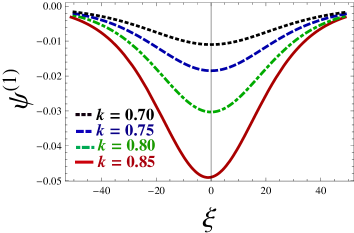
   Figure 7: The variation of the negative potential GS solitons with $k$. The other parameters are fixed at $\alpha=0.4$, $\sigma_{i}=1.4$, $\beta=0.4$, and $U_{0}=0.01$.

   

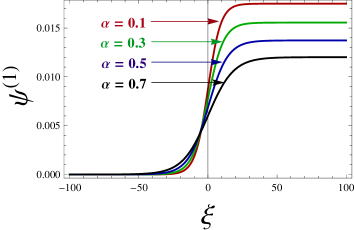
   Figure 8: The variation of the positive potential DLs with $\alpha$ for $k=1.4$, $\sigma_{i}=1.6$, $\beta=0.7$, and $U_{0}=0.01$.

4. In our present attempt we have found the equation of HIA GS which supports both the SWs and DLs solutions by reason of containing both $\psi$-term of K-dV and $\psi^{2}$-term of mK-dV equation. Therefore, the compressive and rarefactive HIA GS solitons are observed to exist above the critical value ($k_{c}>1.48$) and below the critical value ($k_{c}<1.48$) (see Figs. 5-7).

5. The amplitude of the HIA GS increases with the increasing values of spectral index (via $k$) and electron to heavy ion number density (via $\beta$). Besides, the width of the negative potential HIA GS becomes sharper with increases value of $k$ (see Figs. 5-7).

6. It is found that only compressive HIA DLs are exist around critical value ($k>k_{d}$). The amplitude of the positive potential DLs are observed to increase with the decreasing values of ion to heavy ion number density ratio (via $\alpha$) (see Fig. 8).

The principal features of HIA waves in an unmagnetized collisionless EI plasma containing superthermal electrons, Boltzmann distributed light ions, and adiabatic positively charged inertial heavy ions have been theoretically analyzed. We have numerically examined the effects of different plasma parameters on the basic features (viz. polarity, amplitude, and phase speed) of the HIA SWs as well as the adiabatic effects of heavy ions and superthermality effects of electrons. The ranges of plasma parameters used in our investigation ($\alpha=0.1-0.7$, $\sigma_{i}=1.2-2$, $\beta=0.1-0.9$, $\sigma=0.01-0.2$) Jilani2013 ) which are relevant to astrophysical Mendis1994 ; Goertz1989 and labrotory Selwyn1993 ; Winter1998 plasma situations. It is obvious from our present investigation that the effects of superthermal electrons and adiabatic positively charged inertial heavy ions greatly affect the fundamental properties of the HIA SWs.

Lastly, it is clarified from our present attempt that the results that have been found can be useful to know the remarkable features of HIA waves in collisionless unmagnetized plasmas where the effect of superthermality of electrons become pronounced.

Acknowledgments: M. G. Shah, M. M. Rahman and M. R. Hossen are greatly thankful to the Ministry of Science and technology (Bangladesh) for rewarding the National Science and Technology (NST) fellowship.

References

- (1) M. J. Rees, In The Very Early Universe, edited by G.W. Gibbons, S.W. Hawking, and S. Siklas, Cambridge University Press, Cambridge 1983.
- (2) H. R. Miller and P. J. Witta, Active Galactic Nuclei, Springer, Berlin 1987.
- (3) F. C. Michel, Theory of Neutron Star Magnetosphere, Chicago University Press, Chicago 1991.
- (4) O. Havnes, T. Aslaken, F. Melandso, and T. Nitter, Phys. Scr. 45, 491 (1992).
- (5) E. C. Whipple, T. G. Northrop, and D. A. Mendis, J. Geophys. Res. 90, 7405 (1985).
- (6) L. Tonks and I. Langmuir, Phy. Rev. 33, 195 (1929).
- (7) R. W. Revans, Phy. Rev. 44, 798 (1933).
- (8) V. M. Vasyliunas, J. Geophys. Res. 73, 2839 (1968).
- (9) V. Formisano, G. Moreno, and F. Palmiotto, J. Geophys. Res. 78, 3714 (1973).
- (10) J. D. Scudder, E. C. Sittler, and H. S. Bridge, J. Geophys. Res. 86, 8157 (1981).
- (11) W. C. Feldman, R. C. Anderson, J. R. Asbridge, S. J. Bame, J. T. Gosling, et al., J. Geophys. Res. 87, 632 (1982).
- (12) E. Marsch, K. H. Muhlhauser, R. Schwenn, H. Rosenbauer, W. Pilipp, et al., J. Geophys. Res. 87, 52 (1982).
- (13) M. R. Collier, D. C. Hamilton, G. Gloeckler, P. Bochsler, and R. B. Sheldon, Geophys. Res. Lett. 23, 1191 (1996).
- (14) E. E. Antonova, N. O. Ermakova, M. V. Stepanova, M. V. Teltzov, Adv. Space Res. 31, 1229 (2003)
- (15) G. Papp, M. Drevlak, G. I. Pokol, and T. Fulop, J. Plasma Phys. 81, 475810503 (2015).
- (16) L. Zeng, H. R. Koslowski, Y. Liang, A. Lvovskiy, M. Lehnen, et al., J. Plasma Phys. 81, 475810402 (2015).
- (17) T. K. Baluka and M. A. Hellberg, Phys. Plasmas 15, 123705 (2008).
- (18) T. K. Baluku, M. A. Hellberg, I. Kourakis, and N. S. Saini, Phys. Plasmas 17, 053702 (2010).
- (19) A. V. Gurevich, A. V. Lukyanov, and K. P. Zybin, Nucl. Fusion 35, 827 (1995).
- (20) Q. Lu, L. Shan, C. Shen, T. Zhang, Y. Li, et al., J. Geophys. Res. 116, A03224 (2011).
- (21) D. Summers and R. M. Thorne, Phys. Fluids B 3, 1835 (1991).
- (22) T. Cattaert, M. A. Helberg, and R. L. Mace, Phys. Plasmas 14, 082111 (2007).
- (23) M. S. Alam, M. M. Masud, and A. A. Mamun, Plasma Phys. Rep. 39, 1011 (2013).
- (24) B. Basu, Phys. Plasmas 15, 042108 (2008).
- (25) T. K. Baluku and M. A. Hellberg, Phys. Plasmas 19, 012106 (2012).
- (26) C. O. Hines, J. Atmospheric Terrest. Phys. 11, 36 (1957).
- (27) N. N. Rao, P. K. Shukla, and M. Y. Yu, Planet. Space Sci. 38, 543 (1990).
- (28) S. I. Popel and M. Y. Yu, Contrib. Plasma Phys. 35, 103 (1995).
- (29) S. I. Popel, M. Y. Yu, and V. N. Tsytovich, Phys. Plasmas 3, 4313 (1996).
- (30) P. K. Shukla and A. A. Mamun, Introduction to Dusty Plasma Physics, Institute of Physics Publishing, Bristol 2002.
- (31) T. V. Losseva, S. I. Popel, A. P. Golub, and P. K. Shukla, Phys. Plasmas 16, 093704 (2009).
- (32) M. R. Hossen, L. Nahar and A. A. Mamun, Braz. J. Phys. 44, 673 (2014).
- (33) M. R. Hossen, L. Nahar and A. A. Mamun, Braz. J. Phys. 44, 638 (2014).
- (34) M. R. Hossen, S. A. Ema and A. A. Mamun, Commun. Theor. Phys. 62, 888 (2014).
- (35) M. R. Hossen, L. Nahar and A. A. Mamun. J. Astrophys. 2014, 653065 (2014).
- (36) M. R. Hossen and A. A. Mamun, Plasma Sci. Tech. 17, 177 (2015).
- (37) B. Hosen, M. G. Shah, M. R. Hossen and A. A. Mamun, Euro. J. Plus 131, 81 (2016).
- (38) B. Hosen, M. Amina, A. A. Mamun and M. R. Hossen, J. Korean Phys. Soc. 69, 1762 (2016).
- (39) F. Sayed and A. A. Mamun, Phys. Plasmas 14, 034503 (2007).
- (40) S. A. Ema, M. R. Hossen, and A. A. Mamun, Phys. Plasmas 22, 092108 (2015).
- (41) S. A. Ema, M. R. Hossen, and A. A. Mamun, Contrib. Plasma Phys. 55, 596 (2015).
- (42) A. Rahman, F. Sayed, and A. A. Mamun, Phys. Plasmas 14, 034503 (2007).
- (43) A. A. Mamun and N. Jahan, Euro. Phys. Lett. 84, 35001 (2008).
- (44) S. Mahmood and N. Akhtar, Eur. Phys. J. D 49, 217 (2008).
- (45) F. Tanjia and A.A. Mamun, J. Plasma Phys. 75, 99 (2008).
- (46) M. R. Hossen, L. Nahar, S. Sultana, and A. A. Mamun, High Energy Density Phys. 13, 13 (2014).
- (47) M. R. Hossen, L. Nahar, and A. A. Mamun, Phys. Scr. 89, 105603 (2014).
- (48) M. R. Hossen, L. Nahar, S. Sultana, and A. A. Mamun, Astrophys. Space Sci. 353, 123 (2014).
- (49) M. R. Hossen, L. Nahar and, A. A. Mamun, J. Korean Phys. Soc. 65, 1863 (2014).
- (50) D. D. Barbosa and W. S. Kurth, J. Geophys. Res. 85, 6729 (1980).
- (51) T. K. Baluku, M. A. Hellberg, and R. L. Mace, J. Geophys. Res. 116, A04227 (2011).
- (52) M. Shahmansouri, Chin. Phys. Lett. 29, 105201 (2012).
- (53) P. Eslami, M. Mottaghizadeh, and H. R. Pakzad, Phys. Plasmas 18, 072305 (2011).
- (54) P. Eslami, M. Mottaghizadeh, and H. R. Pakzad, Can. J. Phys. 90, 661 (2012).
- (55) M. S. Alam, M. J. Uddin, M. M. Masud, and A. A. Mamun, Chaos 24, 033130 (2014).
- (56) S. Maxon and J. Viecelli, Phys. Rev. Lett. 32, 4 (1974).
- (57) M. G. Shah, M. R. Hossen, and A. A. Mamun, J. Plasma Phys. 81, 905810517 (2015).
- (58) M. G. Shah, M. R. Hossen, S. Sultana, and A. A. Mamun, Chin. Phys. Lett. 32, 085203 (2015).
- (59) M. M. Rahman, M. S. Alam, and A. A. Mamun, Eur. Phys. J. Plus 129, 1 (2014).
- (60) N. C. Lee, Phys. Plasmas 16, 042316 (2009).
- (61) K. Jilani, A. M. Mirza, and T. A. Khan, Astrophys. Space Sci. 344, 135 (2013).
- (62) D. A. Mendis and M. Rosenberg, Annu. Rev. Astron. Astrophys. 32, 419 (1994).
- (63) C. K. Goertz, Rev. Geophys. 27, 271 (1989).
- (64) G. S. Selwyn, Jpn. J. Appl. Phys. 32, 3068 (1993).
- (65) J. Winter, Plasma Phys. Control. Fusion 340, 1201 (1998).