Ion-acoustic solitary pulses in a dense plasma

Abstract

The propagation of ion-acoustic solitary waves (IASWs) in a magnetized, collisionless degenerate plasma system for describing collective plasma oscillations in dense quantum plasmas with relativistically degenerate electrons, oppositely charged inertial ions, and positively charged immobile heavy elements is investigated theoretically. The perturbations of the magnetized quantum plasma are studied employing the reductive perturbation technique to derive the Korteweg-de Vries (K-dV) and the modified K-dV (mK-dV) equations that admits solitary wave solutions. Chandrasekhar limits are used to investigate the degeneracy effects of interstellar compact objects through equation of state for degenerate electrons in case of non-relativistic and ultra-relativistic cases. The basic properties of small but finite-amplitude IASWs are modified significantly by the combined effects of the degenerate electron number density, pair ion number density, static heavy element number density and magnetic field. It is found that the obliqueness affects both the amplitude and width of the solitary waves, whereas the other parameters mainly influence the width of the solitons. The results presented in this paper can be useful for future investigations of astrophysical multi-ion plasmas.

1 Introduction

The study of nonlinear wave phenomena in pair ion plasmas is predominantly significant due to its application in space and laboratory plasmas [1, 2, 3, 4, 5, 6, 7]. Generally, pair ion plasma system is a system containing more than one types of ions and has a great importance to different field of plasma science and technology. The evolution of solitons in plasma having both positive and negative ion species have been investigated by Rizzato et al. [8]. In different laboratory situations, (viz. plasma processing reactors, neutral beam sources, low-temperature laboratory experiments, etc.) the existence of positive-negative ion plasmas has also been found [9, 10, 11]. In addition, a new experimental setup is developed for ion energy loss measurements in a partially ionized, moderately coupled carbon dense plasma with the presence of heavy ion beam [12]. Therefore, the study of plasma excitations in magnetized dense plasmas allow us learning different basic wave phenomena, such as solitons, shock waves, double layers, vortices, etc. One of the basic wave processes namely ion-acoustic (IA) waves in celestial as well as terrestrial plasma system have been studied for several decades both theoretically and experimentally [13, 14, 15, 16, 17, 18, 19, 20, 21]. Washimi and Taniuti [13] were the first to derive the Korteweg de-Vries (KdV) equation governing the propagation of IA waves in a collisionless plasma. IA waves have been studied in various cases, i.e., multi-ion plasma compositions [18, 22], two temperature electron plasmas [17, 22, 23, 24, 25], plasma with superthermal electrons [26, 27], pair-ion plasmas [19, 28], degenerate plasmas [29] and relativistic effect of plasmas [30]. It is well-known that the external magnetic field can modify the propagation properties of the electrostatic IA solitary structures. The effect of an ambient external magnetic field on the electrostatic waves has been studied by a number of authors [31, 32, 33, 34]. Yu et al. [31] extended the Sagdeev approach to study the IA waves in a magnetized plasma. Their results show how the external magnetic field affects the nature of the solitary wave profiles.

Currently, theoretical concerns are to analyze the environment of the compact objects, such as white dwarfs, neutron stars, etc. [35, 36, 37, 38, 39]. The basic constituents of white dwarfs are mainly oxygen, carbon, helium with an envelope of hydrogen gas. The icy satellites of Saturn have been shown to be the source of the heavy positive ion i.e., O⁺, N⁺, etc. plasma in the inner Saturnian torus [40, 41, 42]. The degenerate electron number density in such a compact object is so high (e.g. the degenerate electron number density can be of the order of $10^{30}$ $cm^{-3}$ in white dwarfs, and of the order of $10^{36}$ $cm^{-3}$ in neutron stars) [29, 43] that the electron Fermi energy is comparable to the electron mass energy and the electron speed is comparable to the speed of light in a vacuum. Within astrophysical objects, the lower energy state is filled with electrons so additional electrons cannot give up energy to the lower energy state and they generate degeneracy pressure which is explained by the joined effects of Pauli’s exclusion principle and Heisenberg’s uncertainty principle. The equation of state for degenerate electrons in such interstellar compact objects are explained by Chandrasekhar for two limits where $({P_{e}}\propto{n_{e}}^{5/3})$ for the non-relativistic limit and $({P_{e}}\propto{n_{e}}^{4/3})$ for the ultra-relativistic limit, where $P_{e}$ is the degenerate electron pressure and $n_{e}$ is the degenerate electron number density. To demonstrate the equation of state, Chandrasekhar introduced that for the nonrelativistic degenerate electrons, $\gamma=\frac{5}{3};~{}K=\frac{3}{5}\left(\frac{\pi}{3}\right)^{\frac{1}{3}}\frac{\pi\hbar^{2}}{m}\simeq\frac{3}{5}\Lambda_{c}\hbar c$ where $K$ is the proportionality constant, $\Lambda_{c}=\pi\hbar/mc=1.2\times 10^{-10}~{}cm$, and $\hbar$ is the Planck constant divided by $2\pi$ and for the ultrarelativistic degenerate electrons, $\gamma=\frac{4}{3};~{}K=\frac{3}{4}\left(\frac{\pi^{2}}{9}\right)^{\frac{1}{3}}\hbar c\simeq\frac{3}{4}\hbar c$ [35, 36].

Now, a large number of authors studied the basic properties of solitons or shock waves by deriving the K-dV, mK-dV, Gardner or Burgers equation for planar or nonplanar cases in considering different types of effects [5, 44, 45, 46, 47, 48, 49, 50]. Alinejad and Mamun [28] studied oblique propagation of small amplitude IA solitons in a pair plasma with superthermal electrons. The nonextensivity effects on the obliquely propagating IA waves in a magnetized plasma have been investigated by Shahmansouri and Alinejad [51]. The effect of an applied uniform magnetic field on the propagation of magnetosonic solitary waves in the weakly relativistic limit in a magnetized multi-ion plasma composed of electrons, light ions and heavy ions has been studied by Wang et al. [52]. Masood et al. [53] considered a degenerate quantum magnetized plasma to study the propagation of electromagnetic wave. Hossen et al. [54, 55, 56, 57] investigated the basic features of different nonlinear acoustic waves in the presence of heavy elements in a relativistic degenerate plasma system that is valid only for the unmagnetized case.

To the best of our knowledge, there are no investigations, which have been made for condition of matter by considering magnetized degenerate electrons and oppositely charged ions in a magnetized quantum plasma. Therefore, in this work our main intention is to study the basic features of IASWs by deriving the magnetized K-dV and magnetized mK-dV equations in magnetized dense plasmas.

2 Theoretical model and basic equations

We consider a degenerate, dense, magnetized quantum multi-ion plasma system consisting of both non-relativistic and ultra-relativistic degenerate electrons, non-relativistic degenerate inertial ions of both positively and negatively charged and positively charged immobile heavy elements. It is noted here that the behavior of such a multi-ion plasma may significantly differ from the behavior of a single-ion-species plasma. The study of the effect of magnetic lines of force of both the magnetized positively and negatively charged ions is very common in literature [1, 7, 52, 58, 59, 60]. In equilibrium, we have $n_{e0}+Z_{-}n_{-0}=Z_{+}n_{+0}+Z_{h}n_{h0}$, where $Z_{+}$ is the number of positive ions, $Z_{-}$ is the number of negative ions, $Z_{h}$ is the number of positive ions residing on the heavy ion’s surface and $n_{+0}$, $n_{-0}$, $n_{e0}$ and $n_{h0}$ are the number densities of positive ions, negative ions, electrons and heavy elements in equilibrium. The positively charged static heavy elements participate only in maintaining the quasi-neutrality condition in equilibrium. We consider that the number densities of positive and negative ions is equal in equilibrium i.e., $n_{+0}=n_{-0}$. The dynamics of nonlinear IA waves in the presence of the external magnetic field $\textbf{B}=\hat{z}B_{0}$ is governed by the following momentum equation

$$\nabla\phi-\frac{K_{1}}{n_{e}}\nabla{n_{e}}^{\gamma}=0,$$ (1)

and the non-degenerate inertial ion equations composed of the ion continuity and ion momentum equations are given by

$$\frac{\partial n_{+}}{\partial t}+\nabla.({n_{+}}{\textbf{u}_{+}})=0,$$ (2)

$$\frac{\partial n_{-}}{\partial t}+\nabla.({n_{-}}{\textbf{u}_{-}})=0,$$ (3)

$$\frac{\partial\textbf{u}_{+}}{\partial t}+({\textbf{u}_{+}}.\nabla)u_{+}=-\nabla\phi+\omega_{c_{+}}({\textbf{u}_{+}}\times{\hat{z}}),$$ (4)

$$\frac{\partial\textbf{u}_{-}}{\partial t}+({\textbf{u}_{-}}.\nabla)u_{-}=\beta\nabla\phi+\omega_{c_{-}}({\textbf{u}_{-}}\times{\hat{z}}),$$ (5)

The equation that is closed by Poisson s equation

$$\nabla^{2}\phi=\delta{n_{e}}+\sigma{n_{-}}-{n_{+}}-{Z_{h}}\mu,$$ (6)

where $n_{+}$, $n_{-}$ and $n_{e}$ is the perturbed number densities of inertial positive ions, inertial negative ions and degenerate electrons, respectively). $\textbf{u}_{i}$ is the plasma species fluid speed normalized by $C_{pm}=(m_{e}c^{2}/Z_{p}m_{p})^{1/2}$ with $m_{e}$ ($m_{p}$) being the electron (plasma ion specie s) rest mass, $c$ is the speed of light in vacuum, $\phi$ is the electrostatic wave potential normalized by $m_{e}c^{2}/e$ with e being the magnitude of the charge of an electron. Here $\beta=(Z_{-}m_{+}/Z_{+}m_{-})$ is the ratio of the masses of the positive and the negative ion multiplied by their charge per ion $Z_{s}$ (where s = +, -), $\delta\ =(n_{e0}/Z_{+}n_{+0})$ is the ratio of the number density of electron and positive ion multiplied by charge per positive ion $Z_{+}$, $\sigma=(Z_{-}n_{-0}/Z_{+}n_{+0})$ is the ratio of number density of negative and positive ion multiplied by their charge per ion and $\mu=(n_{h0}/Z_{+}n_{+0})$ is the ratio of the number density of heavy element and positive ion multiplied by $Z_{+}$. The nonlinear propagation of usual IA waves in electron-ion plasma can be recovered by setting $\mu=0$. The time variable ($t$) is normalized by ${\omega_{pm}}=(4\pi n_{p0}e^{2}/m_{p})^{1/2}$, and the space variable ($x$) is normalized by $\lambda_{m}=(m_{e}c^{2}/4\pi n_{p0}e^{2})^{1/2}$. We have defined the parameter that appears in Eq. (1) as $K=n_{e0}^{\gamma-1}K_{e}/{m_{e}}{c}^{2}$.

3 Derivation of the Magnetized K-dV Equation

In order to investigate the dynamics of small but finite amplitude obliquely propagating IA waves in the relativistic degenerate dense magnetized multi-ion quantum plasma, we use the standard reductive perturbation technique to drive the K-dV equation. We now introduce the new set of stretched coordinates as

$$\eta=\epsilon^{1/2}(L_{x}x+L_{y}y+L_{z}z-V_{p}t),$$ (7)

$$T={\epsilon}^{3/2}t,$$ (8)

where $\epsilon$ is a smallness parameter $(0<\epsilon<1)$ measuring the amplitude of perturbation, $V_{p}$ is the wave phase velocity normalized by the IA speed ($C_{im}$), and $l_{x}$, $l_{y}$, and $l_{z}$ are the directional cosines of the wave vector k along the x, y, and, z axes, respectively, so that $l_{x}^{2}$ + $l_{y}^{2}$ + $l_{z}^{2}$ = 1. It is noted here that x, y, z are all normalized by the Debye length $\lambda_{D}$, and $T$ is normalized by the inverse of ion plasma frequency ($\omega_{pi}^{-1}$ ). We may expand $n_{s}$, $u_{s}$, and $\phi$ in power series of $\epsilon$ as

$$n_{s}=1+\epsilon n_{s}^{(1)}+\epsilon^{2}n_{s}^{(2)}+\cdot\cdot\cdot,$$ (9)

$$u_{ix,y}=0+\epsilon^{3/2}u_{ix,y}^{(1)}+\epsilon^{2}u_{ix,y}^{(2)}+\cdot\cdot\cdot,$$ (10)

$$u_{iz}=0+\epsilon u_{iz}^{(1)}+\epsilon^{2}u_{iz}^{(2)}+\cdot\cdot\cdot,$$ (11)

$$\phi=0+\epsilon\phi^{(1)}+\epsilon^{2}\phi^{(2)}+\cdot\cdot\cdot,$$ (12)

Now, substituting Eqs. (7) - (12) into Eqs. (1) - (6) and taking the lowest order coefficient of $\epsilon$, we obtain, $u_{+z}^{(1)}={L_{z}\phi^{(1)}}/{V_{p}}$, $u_{-z}^{(1)}={-L_{z}\beta\phi^{(1)}}/{V_{p}}$, $n_{+}^{(1)}={L_{z}^{2}\phi^{(1)}}/{V_{p}^{2}}$, $n_{-}^{(1)}={-L_{z}^{2}\beta\phi^{(1)}}/{V_{p}^{2}}$, $n_{e}^{(1)}=\phi^{(1)}/K_{11}$, and $V_{p}=L_{z}\sqrt{{\frac{K_{11}(\sigma\beta+1)}{\delta}}}$ represents the dispersion relation for the IA waves that move along the propagation vector $k$.

To the lowest order of x- and y-component of the momentum equations (4) and (5) we get,

$$u_{+y}^{(1)}=\frac{L_{x}}{\omega_{c+}}\frac{\partial\phi^{(1)}}{\partial\eta},$$ (13)

$$u_{+x}^{(1)}=-\frac{L_{y}}{\omega_{c+}}\frac{\partial\phi^{(1)}}{\partial\eta},$$ (14)

$$u_{-y}^{(1)}=-\beta\frac{L_{x}}{\omega_{c-}}\frac{\partial\phi^{(1)}}{\partial\eta},$$ (15)

$$u_{-x}^{(1)}=\beta\frac{L_{y}}{\omega_{c-}}\frac{\partial\phi^{(1)}}{\partial\eta},$$ (16)

Now, substituting Eqs. (7)-(16) into (4) and (5) one can obtain from the higher order series of $\epsilon$ of the momentum and Poisson’s equations as

$$u_{+y}^{(2)}=\frac{L_{y}V_{P}}{\omega_{c+}^{2}}\frac{\partial^{2}\phi^{(1)}}{\partial\eta^{2}},$$ (17)

$$u_{+x}^{(2)}=\frac{L_{x}V_{P}}{\omega_{c+}^{2}}\frac{\partial^{2}\phi^{(1)}}{\partial\eta^{2}},$$ (18)

$$u_{-y}^{(2)}=-\beta\frac{L_{y}V_{P}}{\omega_{c-}^{2}}\frac{\partial^{2}\phi^{(1)}}{\partial\eta^{2}},$$ (19)

$$u_{-x}^{(2)}=-\beta\frac{L_{x}V_{P}}{\omega_{c-}^{2}}\frac{\partial^{2}\phi^{(1)}}{\partial\eta^{2}},$$ (20)

$$\frac{\partial^{2}\phi^{(1)}}{\partial\eta^{2}}=\delta n_{e}^{(2)}+\sigma n_{-}^{(2)}-n_{+}^{(2)},$$ (21)

Using the same process, we get the next higher order continuity equation as well as the z-component of the momentum equation. Now, combining these higher order equations together with Eqs. (13)-(21) one can obtain

$$\frac{\partial\phi^{(1)}}{\partial T}+\lambda\phi^{(1)}\frac{\partial\phi^{(1)}}{\partial\eta}+\beta\frac{\partial^{3}\phi^{(1)}}{\partial\eta^{3}}=0,$$ (22)

This is well-known K-dV equation that describes the obliquely propagating IA waves in a magnetized quantum plasma.

where

$$\lambda=\frac{K_{11}V_{p}}{2\delta}\left[\frac{{\delta}(\gamma-2)}{K_{11}^{2}}-\frac{{3\sigma\beta^{2}L_{z}^{4}}}{V_{p}^{4}}+\frac{3L_{z}^{4}}{V_{p}^{4}}\right]$$ (23)

$$\beta=\frac{K_{11}V_{p}}{2\delta}\left[1+\frac{\sigma\beta(1-L_{z}^{2})}{\omega_{c-}^{2}}+\frac{(1-L_{z}^{2})}{\omega_{c+}^{2}}\right]$$ (24)

In order to indicate the influence of different plasma parameters on the propagation of solitary waves in magnetized quantum plasma, we derive the solution of K-dV equation (22). The stationary solitary wave solution of standard K-dV equation is obtained by considering a frame $\xi=\eta-u_{0}T$ (moving with speed $u_{0}$) and the solution is,

$${\rm\phi^{(1)}}=\rm\phi_{m}{\rm[sech^{2}}(\frac{\xi}{\Delta})],$$ (25)

where the amplitude, $\phi_{m}=3u_{0}/\lambda$, and the width, $\Delta=(4\beta/u_{0})^{1/2}$

4 Derivation of the Magnetized mK-dV Equation

To obtain the mK-dV equation, the same stretched co-ordinates are applied as we used in K-dV equation in section 3 (i.e., Eqs.(7) and (8)) and also used the dependent variables which are expanded as

$$n_{s}=1+\epsilon^{1/2}n_{s}^{(1)}+\epsilon n_{s}^{(2)}+\epsilon^{3/2}n_{s}^{(3)}+\cdot\cdot\cdot,$$ (26)

$$u_{ix,y}=0+\epsilon u_{ix,y}^{(1)}+\epsilon^{3/2}u_{ix,y}^{(2)}+\epsilon^{2}u_{ix,y}^{(3)}+\cdot\cdot\cdot,$$ (27)

$$u_{iz}=0+\epsilon^{1/2}u_{iz}^{(1)}+\epsilon u_{iz}^{(2)}+\epsilon^{3/2}u_{iz}^{(3)}+\cdot\cdot\cdot,$$ (28)

$$\phi=0+\epsilon^{1/2}\phi^{(1)}+\epsilon\phi^{(2)}+\epsilon^{3/2}\phi^{(3)}+\cdot\cdot\cdot,$$ (29)

We find the same expressions for $n_{+}^{(1)}$, $n_{-}^{(1)}$, $n_{e}^{(1)}$, $u_{+z}^{(1)}$, $u_{-z}^{(1)}$, $u_{+x,y}^{(1)}$, $u_{-x,y}^{(1)}$, $u_{+x,y}^{(2)}$, $u_{-x,y}^{(2)}$ and $V_{p}$ by using the values of $\eta$ and $T$ in Eqs.(1)-(6) and (26)-(29) as before in section III. The next higher order series of $\epsilon$ of continuity, momentum and poisson’s equations as

$$\frac{\partial n_{+}^{(1)}}{\partial T}-V_{p}\frac{\partial n_{+}^{(3)}}{\partial\eta}+L_{x}\frac{\partial u_{+x}^{(2)}}{\partial\eta}+L_{x}\frac{\partial}{\partial\eta}(n_{+}^{(1)}u_{+x}^{(1)})+L_{y}\frac{\partial u_{+y}^{(2)}}{\partial\eta}$$

$$+L_{y}\frac{\partial}{\partial\eta}(n_{+}^{(1)}u_{+y}^{(1)})+L_{z}\frac{\partial u_{+z}^{(3)}}{\partial\eta}+L_{z}\frac{\partial}{\partial\eta}(n_{+}^{(1)}u_{+z}^{(2)})+L_{z}\frac{\partial}{\partial\eta}(n_{+}^{(2)}u_{+z}^{(1)})=0,$$ (30)

$$\frac{\partial n_{-}^{(1)}}{\partial T}-V_{p}\frac{\partial n_{-}^{(3)}}{\partial\eta}+L_{x}\frac{\partial u_{-x}^{(2)}}{\partial\eta}+L_{x}\frac{\partial}{\partial\eta}(n_{-}^{(1)}u_{-x}^{(1)})+L_{y}\frac{\partial u_{-y}^{(2)}}{\partial\eta}$$

$$+L_{y}\frac{\partial}{\partial\eta}(n_{-}^{(1)}u_{-y}^{(1)})+L_{z}\frac{\partial u_{-z}^{(3)}}{\partial\eta}+L_{z}\frac{\partial}{\partial\eta}(n_{-}^{(1)}u_{-z}^{(2)})+L_{z}\frac{\partial}{\partial\eta}(n_{-}^{(2)}u_{-z}^{(1)})=0,$$ (31)

$$\hskip 34.1433pt\frac{\partial u_{+z}^{(1)}}{\partial T}-V_{p}\frac{\partial u_{+z}^{(3)}}{\partial\eta}+L_{z}\frac{\partial}{\partial\eta}(u_{+z}^{(1)}u_{+z}^{(2)})+L_{z}\frac{\partial\phi^{(3)}}{\partial\eta}=0,$$ (32)

$$\hskip 34.1433pt\frac{\partial u_{-z}^{(1)}}{\partial T}-V_{p}\frac{\partial u_{-z}^{(3)}}{\partial\eta}+L_{z}\frac{\partial}{\partial\eta}(u_{-z}^{(1)}u_{-z}^{(2)})-L_{z}\beta\frac{\partial\phi^{(3)}}{\partial\eta}=0,$$ (33)

$$\hskip 45.5244ptL_{z}\frac{\partial\phi^{(3)}}{\partial\eta}-K_{11}L_{z}\frac{\partial n_{e}^{(3)}}{\partial\eta}-F\frac{\partial}{\partial\eta}(n_{e}^{(1)}n_{e}^{(2)})=0,$$ (34)

$$\hskip 62.59605pt\frac{\partial^{2}\phi^{(1)}}{\partial\eta^{2}}=\delta n_{e}^{(3)}+\sigma n_{-}^{(3)}-n_{+}^{(3)},$$ (35)

where $F=K_{11}L_{z}(\gamma-2)$

Now combining these higher order equations together with Eqs.(30)-(35) one can obtain

$$\frac{\partial\phi^{(1)}}{\partial T}+M\phi^{(1)2}\frac{\partial\phi^{(1)}}{\partial\eta}+N\frac{\partial^{3}\phi^{(1)}}{\partial\eta^{3}}=0,$$ (36)

This is well-known mK-dV equation that describes the obliquely propagating IA waves in a magnetized multi-ion quantum plasma. where $M$ and $N$ are given by

$$M=\frac{K_{11}V_{p}}{2\delta}\left[\frac{5L_{z}^{6}\beta^{3}\sigma}{6V_{p}^{6}}+\frac{5L_{z}^{6}}{6V_{p}^{6}}-\frac{\delta(\gamma-2)^{2}}{9K_{11}^{3}}\right],$$ (37)

$$N=\frac{K_{11}V_{p}}{2\delta}\left[1+\frac{\sigma\beta(1-L_{z}^{2})}{\omega_{c-}^{2}}+\frac{(1-L_{z}^{2})}{\omega_{c+}^{2}}\right]$$ (38)

The stationary solitary wave solution of the standard mK-dV equation is obtained by considering a frame $\xi=\eta-u_{0}T$ (moving with speed $u_{0}$) and the solution is,

$${\rm\phi^{(1)}}=\rm\phi_{m}{\rm[sech}(\frac{\xi}{\varpi})],$$ (39)

where the amplitude, $\phi_{m}=\sqrt{(6u_{0}/M)}$ and the width $\varpi={\sqrt{(N/u_{0})}}$.

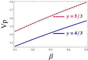
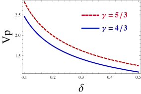
(a)                                (b)

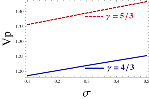
(c)

Figure 1: (Color online) Showing the variation of phase speed $V_{p}$ with (a) the ratio of the masses of the negative and the positive ion multiplied by their charge per ion $\beta$, (b) the ratio of the number density of electrons and positive ions multiplied by charge per positive ion $\delta$, and (c) the ratio of number density of negative and positive ions multiplied by their charge per ion $\sigma$, for $\theta=10^{0}$. The red dashed line represents the non-relativistic case and the blue solid line represents the ultra-relativistic case.

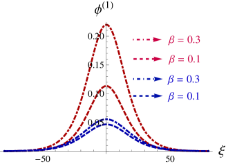
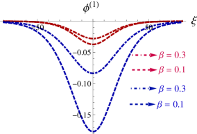
(a)                                                                             (b)

Figure 2: (Color online) Showing the variation of the positive and negative potential K-dV solitons $\phi^{(1)}$ with $\beta$ for $u_{0}=0.01$, $\omega_{ci}=0.5$, $\delta=0.3$, and $\theta=8^{0}$ in case of both non-relativistic and ultra-relativistic limit, where (a) for $\sigma<\sigma_{c}$ and (b) for $\sigma>\sigma_{c}$. The blue line represents the non-relativistic case and the red line represents the ultra-relativistic case.

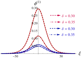
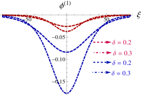
(a)                                                                             (b)

Figure 3: (Color online) Showing the variation of the positive and negative potential K-dV solitons $\phi^{(1)}$ with $\delta$ for $u_{0}=0.01$, $\omega_{ci}=0.5$, $\beta=0.3$, and $\theta=8^{0}$ in case of both non-relativistic and ultra-relativistic limit, where (a) for $\sigma<\sigma_{c}$ and (b) for $\sigma>\sigma_{c}$. The Blue line represents the non-relativistic case and the Red line represents the ultra-relativistic case.

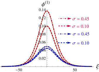
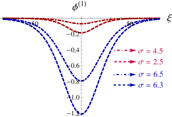
(a)                                                                             (b)

Figure 4: (Color online)(a) Showing the amplitude variation of the K-dV solitons $\phi^{(1)}$ with $\sigma$ for $u_{0}=0.01$, $\omega_{ci}=0.5$, and $\theta=8^{0}$ in case non-relativistic limit and (b) Showing the contour plot of K-dV solitons potential $\phi^{(1)}$ with $\sigma$ for $u_{0}=0.01$, $\omega_{ci}=0.5$, and $\theta=8^{0}$ in case non-relativistic limit.

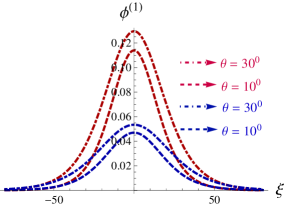
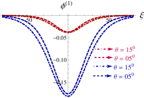
(a)                                                                             (b)

Figure 5: (Color online) Showing the variation of the positive and negative potential K-dV solitons $\phi^{(1)}$ with $\theta$ for $u_{0}=0.01$, $\omega_{ci}=0.5$, $\beta=0.3$ and $\delta=0.3$ in case of both non-relativistic and ultra-relativistic limit, where (a) for $\sigma<\sigma_{c}$ and (b) for $\sigma>\sigma_{c}$. The Blue line represents the non-relativistic case and the Red line represents the ultra-relativistic case.

5 DISCUSSION AND RESULTS

The propagation of IASWs in a magnetized plasma containing of both non-relativistic and ultra-relativistic degenerate electrons, non-relativistic degenerate inertial ions of both positively and negatively charged, and positively charged immobile heavy elements has been studied numerically. To drive K-dV and mK-dV equation we used the well-known reductive perturbation method and then we have studied and analyzed the IASWs solution. We observed and analyzed that both compressive and rarefactive solitary waves (SWs) are found to exist. We have investigate the effects of the different intrinsic parameters (namely the ratio of the masses of the negative and the positive ion multiplied by their charge per ion $\beta$, the ratio of the number density of electrons and positive ions multiplied by charge per positive ions $\delta$, the ratio of number density of negative and positive ion multiplied by their charge per ion $\sigma$, obliqueness $\theta$, cyclotron frequency $\omega_{ci}$, relativistic factor ) on the dynamic properties of IASWs. The amplitude of SWs has been modified by the degenerate pressure of electrons illustrated from the non-relativistic $({P_{e}}\propto{n_{e}}^{5/3})$ to ultra-relativistic $({P_{e}}\propto{n_{e}}^{4/3})$ regime. Adopting Chandrasekhar’s equation of state for relativistically degenerate electrons, it has been examined that the relativistic factor greatly affects the speed of IASWs where for the nonrelativistic degenerate electrons, $\gamma=\frac{5}{3}$ and for the ultrarelativistic degenerate electrons, $\gamma=\frac{4}{3}$, and thus found that the relativistic factor, $\gamma=5/3~{}(nonrelativistic)>\gamma=4/3~{}(ultrarelativistic)$ in every cases.

Here we have numerically obtained that for $\lambda=0$, the amplitude of the K-dV solitons become infinitely large, and the K-dV solution is no longer valid at $\lambda\simeq 0$. It has been observed that the solution of the K-dV equation supports both compressive (positive) and rarefactive (negative) structures depending on the critical value of $\sigma$. In our present investigation, we have found that for $\sigma_{c}=1.70592$, the amplitude of the SWs breaks down due to the vanishing of the nonlinear coefficient $\lambda$. We have observed that at $\sigma<1.70592$, positive (compressive) potential SWs exist, whereas at $\sigma>1.70592$, negative (rarefactive) SWs exist (shown in Figs. 2-4).

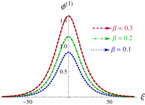
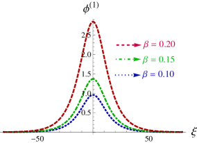
(a)                                                                             (b)

Figure 6: (Color online) Showing the variation of the amplitude of magnetized mK-dV solitons with $\beta$, where (a) for non-relativistic limit and (b) for ultra-relativistic limit. The other plasma parameters are kept fixed.

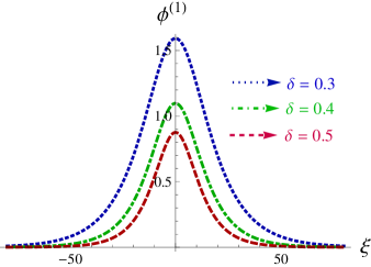
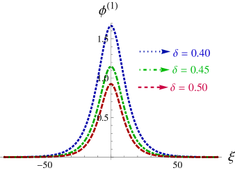
(a)                                                                             (b)

Figure 7: (Color online) (a) Showing the amplitude variation of the mK-dV solitons $\phi^{(1)}$ with $\delta$ for non-relativistic limit and (b) Showing the contour plot of mK-dV solitons potential $\phi^{(1)}$ with $\delta$ for non-relativistic limit.

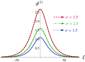
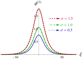
(a)                                                                             (b)

Figure 8: (Color online) Showing the variation of the amplitude of magnetized mK-dV solitons with $\sigma$, where (a) for non-relativistic limit and (b) for ultra-relativistic limit. The other plasma parameters are kept fixed.

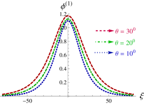
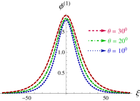
(a)                                                                             (b)

Figure 9: (Color online) Showing the variation of the amplitude of magnetized mK-dV solitons with $\theta$, (a) for non-relativistic limit and (b) for ultra-relativistic limit. The other plasma parameters are kept fixed.

Figure 1 shows the variation of phase speed $V_{p}$ with (a) the ratio of the masses of the negative and the positive ion multiplied by their charge per ion $\beta$. We observed that the phase speed $V_{p}$ increases with the increasing values of $\beta$. (b) the ratio of the number density of electron and positive ion multiplied by charge per positive ion $\delta$. It is shown that with the increase of $\delta$ the phase speed $V_{p}$ decreasing gradually. (c) the ratio of number density of negative and positive ions multiplied by their charge per ion $\sigma$. We found that the phase speed $V_{p}$ increases with the increasing values of $\sigma$. These outcomes are also clear from the phase speed equation of our considered model. It is obvious that the phase speed is always higher for non-relativistic case than those for the ultra-relativistic case. It is due to the variation of the values of the relativistic $\gamma$ factor which is described in introduction.

The effect of $\beta$ on the amplitude of K-dV soliton has shown in Figure 2. It is shown that the amplitude and width of K-dV soliton increases with the increasing values of $\beta$ for both non-relativistic and ultra-relativistic case. Actually, this happens because it increases both the dispersive coefficient and the nonlinearity coefficient. We also found that for positive K-dV soliton $\sigma<\sigma_{c}$ and for negative K-dV soliton $\sigma>\sigma_{c}$.

Figure 3 shows the effect of the variation of $\delta$ with the amplitude of K-dV soliton. It is observed that the solitary profile decreases with increasing values of $\delta$. The effect of $\sigma$ on the amplitude of K-dV soliton was shown in Figure 4. Here we observed that the K-dV soliton increases with the increasing values of $\sigma$. Physically, as the total value of dispersive coefficent increases (i.e., increasing in dispersion of the system), the potential of the solitons increases.

It is shown that the width of the K-dV solitary profiles decrease with the increasing values of $\omega_{ci}$ both for non-relativistic and ultra-relativistic cases. We also observed that the width of the K-dV solitary profile is higher when the plasma system being non-relativistic degenerate case than the ultra-relativistic degenerate case shown in Figure 5 where the width goes to zero when the obliqueness tends to zero and not valid for $\theta>90^{0}$.

Figure 6 shows the effect of obliqueness of the propagation direction, as expressed via $\theta$, is observed for relativistically degenerate electrons, considering $\gamma=5/3$ and $\gamma=4/3$. The variation of amplitude of IASWs is taken place with different values of obliqueness of the wave propagation. It is seen that the amplitude of the magnetized K-dV and mK-dV solitons increases with the increasing of obliqueness, i.e., the angle ($\theta$) between the direction of wave propagation and the magnetic field, $B_{0}$. It is seen that as the value of $\theta$ increases, the amplitude of the solitary waves increases, while their width increases for the lower range of $\delta$ (from $0^{\circ}$ to about $55^{\circ}$), and decreases for its higher range (from $55^{\circ}$ to about $90^{\circ}$). As $\delta\rightarrow 90^{\circ}$, the width goes to $0$, and the amplitude goes to $\infty$. It is likely that for large angles, the assumption that the waves are electrostatic is no longer valid, and we should look for fully electromagnetic structures. Our present investigation is only valid for small value of $\delta$ but invalid for arbitrary large value of $\theta$. In case of larger values of $\theta$, the wave amplitude becomes large enough to break the validity of the reductive perturbation method.

For mK-dV solitons, only compressive solitons are exists which is well-known in plasma literature. It is observed that like K-dV soliton the amplitude of magnetized mK-dV solitons increase with with the increasing of $\beta$ shown in Figure 6. This occurs because $\beta$ increases both the dispersive coefficient and the nonlinearity coefficient. It is also investigated that the amplitude of the mK-dV solitary profiles decreases with the increasing values of $\delta$ as K-dV solitons shown in Figure 7. From Figure 8 we found that for both non-relativistic and ultra-relativistic cases the amplitude of mK-dV solitons increase with the increasing values of $\sigma$. From Figure 9 we found that with the increase in obliqueness the amplitude of magnetized mK-dV solitons increase like K-dV soliton. Actually, the increasing or decreasing of physical parameters strongly responsible for the variation of both the dispersive coefficient (produce due to the dispersion) and the nonlinearity coefficient which makes the solitary strength high or low.

In conclusion, the results of the present investigation should be useful for understanding the nonlinear features of IASWs in a relativistic degenerate quantum multi-ion plasmas which are found in a number of astrophysical plasma systems, such as, neutron stars, white dwarfs, etc. where presence of heavy elements, obliqueness of wave propagation, and relativistic degenerate electrons play a crucial role.

References

- [1] R.S. Tiwari, S.R. Sharma, Modulation instability of ion-acoustic waves in a multi-ion plasma, Phys. Lett. A 77 (1980) 30.
- [2] N. D’Angelo, Low-frequency electrostatic waves in dusty plasmas, Planet. Space Sci. 38 (1990) 1143.
- [3] Chen Yin-Hua, Lu Wei, Wang Wen-Hao, The nonlinear langmuir waves in a multi-ion-component plasma, Commun. Theor. Phys. 35 (2001) 223.
- [4] Y. Nakamura, Y. Saitou, Observation of ion-acoustic waves in two-ion-species plasmas, Plasma Phys. Controlled Fusion 45 (2003) 759.
- [5] A.A. Mamun, R.A. Cairns, P.K. Shukla, Dust negative ion acoustic shock waves in a dusty multi-ion plasma, Phys. Lett. A 373 (2009) 2355.
- [6] D. Perrone, F. Valentini, S. Servidio, S. Dalena, P. Veltri, Vlasov simulations of multi-ion plasma turbulence in the solar wind, Astrophys. J. 762 (2013) 99.
- [7] M. Shahmansouri, H. Alinejad, M. Tribeche, Multi-ion double layers in a magnetized plasma, Commun. Theor. Phys. 64 (2015) 555.
- [8] F.B. Rizzato, R.S. Schneider, D. Dillenburg, Temperature effects on ion acoustic solitons in plasmas with near critical density of negative ions, Plasma Phys. Control. Fusion 29 (1987) 1127.
- [9] R.A. Gottscho, C.E. Gaebe, Negative ion kinetics in RF glow discharges, IEEE Trans. Plasma Sci. 14 (1986) 92.
- [10] M. Bacal, G.W. Hamilton, H- and D- Production in Plasmas, Phys. Rev. Lett. 42 (1979) 1538.
- [11] J. Jacquinot, B.D. McVey, J.E. Scharer, Mode conversion of the fast magnetosonic wave in a deuterium-hydrogen tokamak plasma, Phys. Rev. Lett. 39 (1977) 88.
- [12] A. Ortner, D. Schumacher, W. Cayzac, A. Frank, M.M. Basko, S. Bedacht, A. Blazevic, S. Faik, D. Kraus, T. Rienecker, G. Schaumann, An. Tauschwitz, F. Wagner and M. Roth, A novel experimental setup for energy loss and charge state measurements in dense moderately coupled plasma using laser-heated hohlraum targets, J. Phys.: Conf. Ser. 688 (2016) 012081.
- [13] H. Washimi, T. Taniuti, Propagation of ion-acoustic solitary waves of small amplitude, Phys. Rev. Lett. 17 (1966) 996.
- [14] R.Z. Sagdeev, Cooperative phenomena and shock waves in collisionless plasmas, Rev. Plasma Phys. 4 (1966) 23.
- [15] H. Ikezi, R.J. Taylor, D.R. Baker, Formation and interaction of ion-acoustic solitions, Phys. Rev. Lett. 25 (1970) 11.
- [16] A. Mase, T. Tsukishima, Measurements of ion wave turbulence by microwave scattering, Phys. Fluids 18 (1975) 464.
- [17] S. Baboolal, R. Bharuthram, Cut-off conditions and existence domains for large-amplitude ion-acoustic solitons and double layers in fluid plasmas, J. Plasma Phys. 44 (1990) 1.
- [18] R. Bharuthram, P.K. Shukla, Large amplitude ion-acoustic solitons in a dusty plasma, Planet. Space Sci. 40 (1992) 973.
- [19] S.I. Popel, S.V. Vladimirov, P.K. Shukla, Ion-acoustic solitons in electron positron ion plasmas, Phys. Plasmas 2 (1995) 716.
- [20] A.A. Mamun, Effects of ion temperature on electrostatic solitary structures in nonthermal plasmas, Phys. Rev. E 55 (1997) 1852.
- [21] A.A. Mamun, P.K. Shukla, Spherical and cylindrical dust acoustic solitary waves. Phys. Lett. A 290 (2001) 173.
- [22] M. Shahmansouri, M. Tribeche, Propagation properties of ion acoustic waves in a magnetized superthermal bi-ion plasma, Astrophys. Space Sci. 350 (2014) 781.
- [23] S. Baboolal, R. Bharuthram, M.A. Hellberg, Arbitrary-amplitude theory of ion-acoustic solitons in warm multi-fluid plasmas, J. Plasma Phys. 41 (1989) 341.
- [24] W.K.M. Rice, M.A. Hellberg, R.L. Mace, S. Baboolal, Finite electron mass effects on ion-acoustic solitons in a two electron temperature plasma, Phys. Lett. A 174 (1993) 416.
- [25] S.S. Ghosh, K.K. Ghosh, A.N. Sekar Iyengar, Large Mach number ion acoustic rarefactive solitary waves for a two electron temperature warm ion plasma, Phys. Plasmas 3 (1996) 3939.
- [26] M.G. Shah, M.M. Rahman, M.R. Hossen, A.A. Mamun, Roles of superthermal electrons and adiabatic heavy ions on heavy-ion-acoustic solitary and shock waves in a multi-component plasma, Commun. Theor. Phys. 64 (2015) 208.
- [27] M.G. Shah, M.M. Rahman, M.R. Hossen, A.A. Mamun, Properties of cylindrical and spherical heavy ion-acoustic solitary and shock structures in a multi-species plasma with superthermal electrons, Plasma Phys. Rep. 42 (2016) 168.
- [28] H. Alinejad, A.A. Mamun, Oblique propagation of electrostatic waves in a magnetized electron-positron-ion plasma with superthermal electrons, Phys. Plasmas 18 (2011) 112103.
- [29] M.R. Hossen, L. Nahar, S. Sultana, A.A. Mamun, Roles of positively charged heavy ions and degenerate plasma pressure on cylindrical and spherical ion acoustic solitary waves, Astrophys. Space Sci. 353 (2014) 123.
- [30] M.G. Shah, M.R. Hossen, S. Sultana, A.A. Mamun, Positron-acoustic shock waves in a degenerate multi-component plasma, Chin. Phys. Lett. 32 (2015) 085203.
- [31] M.Y. Yu, P.K. Shukla, S. Bujarbarua, Fully nonlinear ion-acoustic solitary waves in a magnetized plasma, Phys. Fluids 23 (1980) 2146.
- [32] P.K. Shukla, A.A. Mamun, Dust-acoustic shocks in a strongly coupled dusty plasma, IEEE Trans. Plasma Sci. 29 (2001) 221.
- [33] A.A. Mamun, M.N. Alam, A.K. Das, Z. Ahmed, T.K. Datta, Obliquely propagating electrostatic solitary structures in a hot magnetized dusty plasma, Phys. Scr. 58 (1998) 72.
- [34] S. Sultana, I. Kourakis, M.A. Hellberg, Oblique propagation of arbitrary amplitude electron acoustic solitary waves in magnetized kappa-distributed plasmas, Plasma Phys. Controlled Fusion 54 (2012) 105016.
- [35] S. Chandrasekhar, The density of white dwarf stars, Philos. Mag. 11 (1931) 592.
- [36] S. Chandrasekhar, The highly collapsed configurations of a stellar mass, Mon. Not. R. Astron. Soc. 170 (1935) 405.
- [37] S.L. Shapiro, S.A. Teukolsky, Black Holes, White Dwarfs and Neutron Stars: The Physics of Compact Objects : John Wiley & Sons, New York, 1983.
- [38] M.G. Shah, Quantum positron-acoustic waves in dense plasmas (Lap-lambert Publishing, Germany, 2015). ISBN- 978-3-659-81624-6
- [39] M.G. Shah, M.R. Hossen, A.A. Mamun, Nonlinear propagation of positron-acoustic waves in a four component space plasma, J. Plasma Phys. 81 (2015) 905810517.
- [40] A. Eviatar, R.L. Mcnutt, G.L. Siscoe, J.D. Sullivan, Heavy ions in the outer Kronian magnetosphere, J. Geophys. Res. 88 (1983) 823.
- [41] J.D. Richardson, Thermal ions at Saturn: Plasma parameters and implications, J. Geophys. Res. 91 (1986) 1381.
- [42] S.A. Ema, M.R. Hossen, A.A. Mamun, Nonplanar shocks and solitons in a strongly coupled adiabatic plasma: the roles of heavy ion dynamics and nonextensitivity, Cotrib. Plasma Phys. 55 (2015) 596.
- [43] M.R. Hossen, L. Nahar, A.A. Mamun, Roles of arbitrarily charged heavy ions and degenerate plasma pressure in cylindrical and spherical IA shock waves, Phys. Scr. 89 (2014) 105603.
- [44] P. Chatterjee, D.K. Ghosh, B. Sahu, Planar and nonplanar ion acoustic shock waves with nonthermal electrons and positrons, Astrophys. Space Sci. 339 (2012) 261.
- [45] A. Mannan, A.A. Mamun, Planar electron-acoustic solitary waves and double layers in a two-electron-temperature plasma with nonthermal ions, Astrophys. Space Sci. 340 (2012) 109.
- [46] W.F. El-Taibany, M. Wadati, Nonlinear quantum dust acoustic waves in nonuniform complex quantum dusty plasma, Phys. Plasmas 14 (2007) 042302.
- [47] M.S. Zobaer, N. Roy, A.A. Mamun, DIA solitary and shock waves in dusty multi-ion dense plasma with arbitrary charged dust, J. Mod. Phys. 3 (2012) 755.
- [48] U.K. Samanta, A. Saha, P. Chatterjee, Bifurcations of nonlinear ion acoustic travelling waves in the frame of a Zakharov-Kuznetsov equation in magnetized plasma with a kappa distributed electron, Phys. Plasmas 20 (2013) 052111.
- [49] A. Saha, N. Pal, P. Chatterjee, Dynamic behavior of ion acoustic waves in electron-positron-ion magnetoplasmas with superthermal electrons and positrons, Phys. Plasmas 21 (2014) 102101.
- [50] M.G. Shah, M.R. Hossen, A.A. Mamun, Nonplanar positron-acoustic shock waves in astrophysical plasmas, Braz. J. Phys. 45 (2015) 219.
- [51] M. Shahmansouri, H. Alinejad, Effect of electron nonextensivity on oblique propagation of arbitrary ion acoustic waves in a magnetized plasma, Astrophys. Space Sci. 344 (2013) 463.
- [52] Y. Wang, Z. Zhou, Y. Lu, X. Ni, J. Shen, Y. Zhang, Relativistic magnetosonic solitary wave in magnetized multi-ion plasma, Commu. Theor. Phys. 51 (2009) 1121.
- [53] W. Masood, B. Eliasson, P.K. Shukla, Electromagnetic wave equations for relativistically degenerate quantum magnetoplasmas, Phys. Rev. E 81 (2010) 066401.
- [54] M.R. Hossen, L. Nahar, S. Sultana, A.A. Mamun, Nonplanar ion-acoustic shock waves in degenerate plasmas with positively charged heavy ions, High Energy density Phys. 13 (2014) 13.
- [55] M.R. Hossen, A.A. Mamun, Electrostatic solitary structures in a relativistic degenerate multispecies plasma, Braz. J. Phys. 44 (2014) 673.
- [56] M.R. Hossen, S.A. Ema, A.A. Mamun, Nonplanar shock structures in a relativistic degenerate multi-species plasma, Commun. Theor. Phys. 62 (2014) 888.
- [57] M.R. Hossen, A.A. Mamun, Nonplanar shock excitations in a four component degenerate quantum plasma: the effects of various charge states of heavy ions, Plasma Sci. Technol. 17 (2015) 177.
- [58] N. Chakrabarti, A. Fruchtman, R. Arada, Y. Marona, Ion dynamics in a two-ion-species plasma, Phys. Lett. A 297 (2002) 92.
- [59] D. Tskhakaya, S. Kuhn, Boundary conditions for the multi-ion magnetized plasma-wall transition, J. Nucl. Mater. (2005) .
- [60] M.M. Haider, T. Ferdous, S.S. Duha, The effects of vortex like distributed electron in magnetized multi-ion dusty plasmas, Cent. Eur. J. Phys. 12 (2014) 701.