Nucleus-acoustic solitary waves and double layers in a magnetized degenerate quantum plasma

Abstract

The properties of nucleus-acoustic (NA) solitary waves (SWs) and double layers (DLs) in a four-component magnetized degenerate quantum plasma system (containing non-degenerate inertial light nuclei, both non-relativistically and ultra-relativistically degenerate electrons and positrons, and immobile heavy nuclei) are theoretically investigated by the reductive perturbation method. The Korteweg-de Vries (K-dV), the modified K-dV (MK-dV), and the Gardner equations are derived to examine the basic features (viz. amplitude, speed, and width) of NA SWs and DLs. It is found that the effects of the ultra-relativistically degenerate electrons and positrons, stationary heavy nuclei, external magnetic field (obliqueness), etc. significantly modify the basic features of the NA SWs and DLs. The basic features and the underlying physics of NA SWs and DLs, which are relevant to some astrophysical compact objects including white dwarfs and neutron stars, are pinpointed.

I Introduction

There has been a great deal of interest in understanding the plasma fluid dynamics inside the astrophysical dense electron-positron-ion (EPI) plasmas. The EPI plasma is an omnipresent ingredient of many astrophysical systems or regions, such as early universe Misner1973 , active galactic nuclei Begelman1984 ; Miller1987 ; Tribeche2009 , pulsar magnetosphere Liang1998 ; Michel1982 , white dwarfs Hossen2014a ; Hossen2014b , polar regions of neutron stars Michel1991 , solar atmospheres Goldreich1969 ; Hansen1988 , inner regions of the accretion disc surrounding black holes Rees1971 , center of our galaxy Burns1983 , etc. A number of invesitgations have been made on small amplitude solitons in EPI plasmas in the presence of significant percentage of positrons Popel1995 . The annihilation time of positrons in the plasma is long compared with typical particle confinement times. However, for long lifetime of positrons, different types of linear waves and associated nonlinear structures can be generated in such EPI plasmas Tandberg-Hansen1988 ; Piran1999 . The characteristics of linear waves and nonlinear structures have been influenced considerably due to the presence of positron component along with electrons and ions in most space plasmas.

It is now well established that the effect magnetic field significantly modifies the basic properties of linear and nonlinear waves in EPI plasmas which are, in fact, magnetized for most laboratory, space, and astrophysical situations Matthaeus2005 ; Jehan2008 ; Bains2010 ; Mahmood2003 ; Sabry2012 . The electromagnetic forces and degenerate pressures of electrons and positrons give rise to different types of fluctuations at very short length and time scales. The effect of magnetic field on the stability behaviour of low-frequency electrostatic IA waves in EPI plasmas is examined by Jehan et al. Jehan2008 . Bains et al. Bains2010 studied the modulational instability of IA waves encompasses in magnetized quantum EPI plasmas. The large amplitude IA waves propagation in magnetized EPI plasma using Sagdeev potential approach is studied by Mahmood et al. Mahmood2003 . Sabry et al. Sabry2012 have taken the typical magnetized EPI parameters, which are relevent to white dwarfs and corona of magnetars, to examine the IA freak waves in ultra-relativistic degenerate EPI plasmas.

Recently, there has been a renewed interest in studying the relativistic degenerate dense plasmas due to its existence in interstellar compact objects, such as white dwarfs Zobaer2012 ; Akhter2013 ; mr2014a ; mr2014b , neutron stars Shapiro1983 ; Mamun2010a ; Mamun2010b and in tense laser plasma experiments Marklund2006 ; Mourou2006 . It is observed that at a very large number densities, when the electron and positron Fermi energies become dominant over the electron and positron thermal energies, then the electron-positron thermal pressure can be ignored in comparison with the electron-positron degeneracy pressures. Within a astrophysical objects, the lower energy state is filled of electrons so additional electrons be cannot given up energy to the lower energy state and therefore they generate degeneracy pressure. In case of astrophysical compact object, like white dwarf, the average density could be varied from $10^{6}$ $gmcm^{-3}$ to $10^{8}$ $gmcm^{-3}$, the degenerate electron number can be of the order of $10^{30}$ $cm^{-3}$, and the average inter-particle distance is of the order of $10^{-10}$ $cm$ which is of the order of $10^{-13}$ $cm$ for neutron star Shapiro1983 ; Mamun2010a ; Koester1990 ; Azam2005 . In such compact objects the light nuclei can be assumed to be inertial, whereas the electrons and positrons are taken to follow the degeneracy pressure in order to support these objects against the gravitational collapse. It is notable that the basic constituents of white dwarfs are mainly positively and negatively charged heavy elements like carbon, oxygen, helium with an envelope of hydrogen gas. The existence of heavy elements (positively and negatively) is found to form in a prestellar stage of the evolution of the universe, when all matter was compressed to extremely high densities. The average number density of heavy particles is of the order of $10^{29}$ $cm^{-3}$ where distance between heavy particles is of the order of $10^{-10}$ $cm$ (for white dwarfs) Koester1990 .

A general expression for the degenerate pressure of relativistic ions and electrons is given by Chandrasekhar. The equation of state regarding the degeneracy of plasma species is presented at earlier in case of both the non-relativistic $({P_{f}}\propto{n_{f}}^{5/3})$ and the ultra-relativistic $({P_{f}}\propto{n_{f}}^{4/3})$ limits by Chandrasekhar Chandrasekhar1931 ; Chandrasekhar1935 , where $P_{f}$ shows the degenerate pressure and $n_{f}$ describes the number density of plasma species $f$, respectively. To demonstrate the equation of state, Chandrasekhar introduced that for the nonrelativistic degenerate electrons, $\gamma=\frac{5}{3};~{}K=\frac{3}{5}\left(\frac{\pi}{3}\right)^{\frac{1}{3}}\frac{\pi\hbar^{2}}{m}\simeq\frac{3}{5}\Lambda_{c}\hbar c$ where $K$ is the proportionality constant, $\Lambda_{c}=\pi\hbar/mc=1.2\times 10^{-10}~{}cm$, and $\hbar$ is the Planck constant divided by $2\pi$ and for the ultrarelativistic degenerate electrons, $\gamma=\frac{4}{3};~{}K=\frac{3}{4}\left(\frac{\pi^{2}}{9}\right)^{\frac{1}{3}}\hbar c\simeq\frac{3}{4}\hbar c$. Using the Chandrasekhar limit, Taibany et al. El-Taibany2012 considered an ultra dense plasma to study the properties of electromagnetic perturbation modes (fast and slow modes) and clarified that the roles of degeneracy of electrons and positrons, enthalpy corrections, strength of magnetic field, and relativistic factor greatly modify the magnetosonic perturbation modes. Pakzad and Javidan Pakzad2011 studied the IASWs in dissipative plasmas containing relativitic ions, nonthermal electrons, and maxwellian positrons. Ting et al. Ting1992 thought out a relativistic plasma system with nonisothermal electrons and examined the transient features of solitary waves. Chatterjee et al. Chatterjee2012 analyzed the nonlinear propagation of IASWs in an unmagmetized plasma comprising of nonthermal electrons and positrons, and singly charged adiabatically hot positive ions in planar ana nonplanar geometries. Moslem et al. Moslem2007 studied the two-dimensional non-linear acoustic excitations in EPI plasmas that are applicable to the accretion discs of active galactic nuclei, where the ion temperature are 3-300 times higher than those of electrons. Haque and Saleem Haque2003 studied large amplitude two-dimensional IA and drift wave vortices in magnetized EPI plasmas, where the electrons and positrons were assumed to be Boltzmann-distributed. Masood and Mushtaq Masood2008 investigated the linear properties of obliquely propagating magnetoacoustic waves in EPI quantum magnetoplasmas and found that the corrections significantly modify the propagation of fast and slow magnetoacoustic waves in both plasmas. Rizzato Rizzato1988 studied the localization of weakly nonlinear circularly polarized electromagnetic waves in a cold plasma made up of electrons, positrons, and ions. Shah et al. Shah2015a ; Shah2015b ; Shah2015c ; Shah2015d studied an unmagnetized degenerate quantum plasma and investigated the effects of relativistic degenerate electrons and positrons and plasma particle number densities on the propagation of positron-acoustic solitary or shock waves. Shuchy et al. Shuchy2012 studied the electron-acoustic (EA) and dust-electron-acoustic Gardner Solitons (GSs) and DLs with two-temperature-electron (hot and cold) following Boltzmann distributions. Wang et al. Wang2009 investigated the effect of an external uniform magnetic field on the propagation of solitary waves in a in the weakly relativistic magnetized multi-ion plasma containing electrons and light and heavy ions. Labany and Shaaban Labany1995 have considered nonlinear IA waves in a weakly relativistic plasma consisting of warm ion-fluid with non-isothermal electrons. The propagation of electrostatic and electro-magnatic waves in quantum plasma with relativistic degenerate electrons has been analyzed by Khan Khan2012 . Mamun and Shukla Mamun2010a considered the reductive perturbation technique to investigate the solitary waves in ultra-relativistic degenerate dense plasmas. Zeba et al. Zeba2012 studied the nonlinear IA waves in the dense unmagnetized EPI plasmas with ultra-relativistic degenerate electrons and positrons. Masood et al. Masood2010 studied the electro-magnetic wave equation for relativistic degenerate quantum magnetized plasmas. More recently, Hossen et al. rasel2014a ; rasel2014b ; rasel2014c ; rasel2015 investigated the basic features of different nonlinear acoustic waves in the presence of heavy elements in a relativistic degenerate plasma system. But this attempts is valid only for unmagnetized case. However, to the best of knowledge, no theoretical investigation has been made on the nonlinear properties of NA SWs in magnetized degenerate quantum plasmas with relativistic degenerate electrons and positrons. Therefore, in our present work, we attempt to study the basic features of NA SWs by deriving the K-dV, MK-dV and Gardner equations in magnetized degenerate quantum plasma containing non-degenerate inertial light nuclei, both non-relativistically and ultra-relativistically degenerate electrons and positrons, and immobile heavy nuclei.

The manuscript is organized as follow. The theoretical model describing the dynamics of the NA waves is described in Sec. II. The nonlinear dynamical equation, namely K-dV (MK-dV) Gardner equations and its solitay wave solution are derived and interpreted in Sec. III (IV) V. A brief discussion is finally provided in Sec. VI.

II Theoretical Model

We consider a four component magnetized quantum plasma system consisting of non-degenerate inertial light nuclei, both non-relativistic and ultra-relativistic degenerate electrons and positrons, and immobile heavy nuclei. At equilibrium, $n_{e0}=n_{i0}+n_{p0}+Z_{h}n_{h0}$, where $n_{e0}$, $n_{i0}$, $n_{p0}$ are the unperturbed number densities of degenerate electron, inertial light nuclei, degenerate positron, respectively and $Z_{h}$ is the number of negative ions residing onto the heavy nuclei surface. The positively charged static heavy nuclei participate only in maintaining the quasi-neutrality condition at equilibrium. The mass of the electrons and positrons can be considered inertialess in comparison to light nuclei mass, and one can describe the degenerate pressure through Eqs. (1) and (2). Generally, in a relativistically degenerate plasma system, pressure arises due to the combined effect of Pauli’s exclusion principle and Heisenberg’s uncertainty principle, and depends only on the number density of constituent particles, but not on its thermal temperatures Mamun2010a ; Koester1990 . The electron and positron inertia can in fact be neglected if we consider that NA electrostatic waves move at phase velocity ($V_{p}$) which is much higher than the light nuclei thermal speed and yet in turn much lower than the electron and positron thermal speed: $V_{th,i}<<V_{p}<<V_{th,e,p}$. The dynamics of nonlinear NA waves in the presence of the external magnetic field $\textbf{B}=\hat{z}B_{0}$ is governed by the following momentum equation

$$\nabla\phi-\frac{K_{1}}{n_{e}}\nabla{n_{e}}^{\gamma}=0,$$ (1)

$$\nabla\phi-\frac{K_{2}}{n_{p}}\nabla{n_{p}}^{\gamma}=0,$$ (2)

and the non-degenerate inertial light nuclei equations composed of the light nuclei continuity and light nuclei momentum equations are given by

$$\frac{\partial n_{i}}{\partial t}+\nabla.({n_{i}}{\textbf{u}_{i}})=0,$$ (3)

$$\frac{\partial\textbf{u}_{i}}{\partial t}+({\textbf{u}_{i}}.\nabla)u_{i}=-\nabla\phi+\omega_{ci}({\textbf{u}_{i}}\times{\hat{z}}),$$ (4)

The equation that is closed by Poisson s equation

$$\nabla^{2}\phi={n_{e}}{\alpha_{e}}-n_{i}-{n_{p}}{\alpha_{p}}-{Z_{h}}\mu,$$ (5)

where $n_{s}$ is the perturbed number densities of species s (here s = i, e, p inertial light nuclei, degenerate electron, degenerate positron, respectively). $\textbf{u}_{i}$ is the light nuclei fluid speed normalized by NA speed $C_{i}=(m_{e0}c^{2}/m_{i0})^{1/2}$ with $m_{e0}$ ($m_{i0}$) being the electron (light nuclei) rest mass, $c$ is the speed of light in vacuum, $\phi$ is the electrostatic wave potential normalized by $m_{e0}c^{2}/e$. Here $\mu\ =(n_{h0}/n_{i0})$ is the heavy nuclei to light nuclei number density ratio, $\alpha_{e}=(n_{e0}/n_{i0})$ is the electron to light nuclei number density ratio and $\alpha_{p}=(n_{p0}/n_{i0})$ is the positron to light nuclei number density ratio. The nonlinear propagation of usual NA waves in EPI plasma can be recovered by setting $\mu=0$. The time variable ($t$) is normalized by ${\omega_{pi}}=(4\pi n_{i0}e^{2}/m_{i0})^{1/2}$, and the space variable ($x$) is normalized by $\lambda_{s}=(m_{e0}c^{2}/4\pi n_{i0}e^{2})^{1/2}$. The numerical value of $\lambda_{s}$ is of the order of $10^{-10}cm$ Mamun2010a . We have defined the parameters appeared in Eq. (1) as relativistic factor for degenerate electrons, $K_{1}=n_{e0}^{\gamma-1}K_{e}/{m_{e0}}{c}^{2}$ and in Eq. (2) as relativistic factor for degenerate positrons, $K_{2}=n_{p0}^{\gamma-1}K_{p}/{m_{e0}}{c}^{2}$.

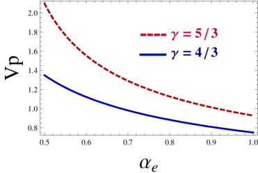
Figure 1: (Color online) Showing the variation of phase speed $V_{p}$ with $\alpha_{e}$ for $u_{0}=0.1$, $\delta=10^{0}$, and $\alpha_{p}=0.2$. The red dashed line represents the non-relativistic case and the blue solid line represents the ultra-relativistic case.

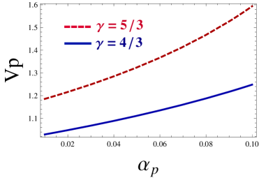
Figure 2: (Color online) Showing the variation of phase speed $V_{p}$ with $\alpha_{p}$ for $u_{0}=0.1$, $\delta=10^{0}$, and $\alpha_{e}=0.4$. The red dashed line represents the non-relativistic case and the blue solid line represents the ultra-relativistic case.

Figure 3: (Color online) Showing the variation of positive potential K-dV solitons with $\alpha_{p}$ for $u_{0}=0.1$, $\alpha_{e}=0.4$, $\omega_{ci}=0.5$, and $\delta=10^{0}$ in case of non-relativistic limit.

Figure 4: (Color online) Showing the variation of positive potential K-dV solitons with $\alpha_{p}$ for $u_{0}=0.1$, $\alpha_{e}=0.4$, $\omega_{ci}=0.5$, and $\delta=10^{0}$ in case of ultra-relativistic limit.

III K-dV Equation

To study the dynamics of small but finite amplitude obliquely propagating NA waves in a magnetized electron-ion (EI) plasma, we apply the reductive perturbation technique in which independent variables are stretched as

$$\eta=\epsilon^{1/2}(L_{x}x+L_{y}y+L_{z}z-V_{p}t),$$ (6)

$$T={\epsilon}^{3/2}t,$$ (7)

where $\epsilon$ is a smallness parameter $(0<\epsilon<1)$ measuring the amplitude of perturbation, $V_{p}$ is the wave phase velocity normalized by the NA speed ($C_{i}$), and $l_{x}$, $l_{y}$, and $l_{z}$ are the directional cosines of the wave vector k along the x, y, and, z axes, respectively, so that $l_{x}^{2}$ + $l_{y}^{2}$ + $l_{z}^{2}$ = 1. It is noted here that x, y, z are all normalized by the Debye length $\lambda_{D}$, and $T$ is normalized by the inverse of light nuclei plasma frequency ($\omega_{pi}^{-1}$ ). We may expand $n_{s}$, $u_{s}$, and $\phi$ in power series of $\epsilon$ as

$$n_{s}=1+\epsilon n_{s}^{(1)}+\epsilon^{2}n_{s}^{(2)}+\cdot\cdot\cdot,$$ (8)

$$u_{ix,y}=0+\epsilon^{3/2}u_{ix,y}^{(1)}+\epsilon^{2}u_{ix,y}^{(2)}+\cdot\cdot\cdot,$$ (9)

$$u_{iz}=0+\epsilon u_{iz}^{(1)}+\epsilon^{2}u_{iz}^{(2)}+\cdot\cdot\cdot,$$ (10)

$$\phi=0+\epsilon\phi^{(1)}+\epsilon^{2}\phi^{(2)}+\cdot\cdot\cdot,$$ (11)

now, applying Eqs. (6)-(11) into Eqs. (1) - (5) and taking the lowest order coefficient of $\epsilon$, we obtain, $u_{iz}^{(1)}={L_{z}\phi^{(1)}}/{V_{p}}$, $n_{i}^{(1)}={L_{z}^{2}\phi^{(1)}}/{V_{p}^{2}}$, $n_{e}^{(1)}=\phi^{(1)}/K_{11}$, $n_{p}^{(1)}=\phi^{(1)}/K_{22}$, and $V_{p}=L_{z}\sqrt{(\frac{{K_{11}}{K_{22}}}{{K_{22}}{\alpha_{e}}-{K_{11}}{\alpha_{p}}})}$ represents the dispersion relation for the NA waves that move along the propagation vector $k$.

To the lowest order of x- and y-component of the momentum equation (4) we get

$$u_{iy}^{(1)}=\frac{L_{x}}{\omega_{ci}}\frac{\partial\phi^{(1)}}{\partial\eta},$$ (12)

$$u_{ix}^{(1)}=-\frac{L_{y}}{\omega_{ci}}\frac{\partial\phi^{(1)}}{\partial\eta}.$$ (13)

Now, applying Eqs. (6)-(13) into (4) one can obtain from the higher order series of $\epsilon$ of the momentum and Poisson’s equations as

$$u_{iy}^{(2)}=\frac{L_{y}V_{P}}{\omega_{ci}^{2}}\frac{\partial^{2}\phi^{(1)}}{\partial\eta^{2}},$$ (14)

$$u_{ix}^{(2)}=\frac{L_{x}V_{P}}{\omega_{ci}^{2}}\frac{\partial^{2}\phi^{(1)}}{\partial\eta^{2}},$$ (15)

$$\frac{\partial^{2}\phi^{(1)}}{\partial\eta^{2}}=n_{e}^{(2)}\alpha_{e}-n_{i}^{(2)}-n_{p}^{(2)}\alpha_{p}.$$ (16)

We now follow the same process to get the next higher order continuity equation as well as z-component of the momentum equation. Combining these higher order equations together with Eqs. (12)-(16) one can obtain the K-dV equation in the form

$$\frac{\partial\phi^{(1)}}{\partial T}+\lambda\phi^{(1)}\frac{\partial\phi^{(1)}}{\partial\eta}+\beta\frac{\partial^{3}\phi^{(1)}}{\partial\eta^{3}}=0,$$ (17)

where

$$\lambda=\frac{V_{p}^{3}}{2L_{z}^{2}}\left[\frac{{\alpha_{e}}(\gamma-2)}{K_{11}^{2}}-\frac{{\alpha_{p}}(\gamma-2)}{K_{22}^{2}}-\frac{3L_{z}^{4}}{V_{p}^{4}}\right],$$ (18)

$$\beta=\frac{V_{p}^{3}}{2L_{z}^{2}}\left[1+\frac{(1-L_{z}^{2})}{\omega_{ci}^{2}}\right].$$ (19)

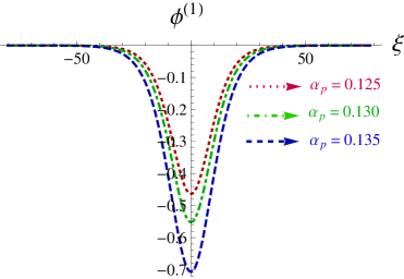
Figure 5: (Color online) Showing the variation of negative potential K-dV solitons with $\alpha_{p}$ for $u_{0}=0.1$, $\alpha_{e}=0.4$, $\omega_{ci}=0.5$, and $\delta=10^{0}$ in case of non-relativistic limit.

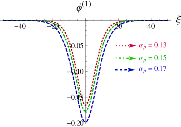
Figure 6: (Color online) Showing the variation of negative potential K-dV solitons with $\alpha_{p}$ for $u_{0}=0.1$, $\alpha_{e}=0.4$, $\omega_{ci}=0.5$, and $\delta=10^{0}$ in case of ultra-relativistic limit.

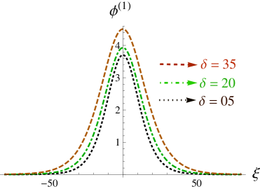
Figure 7: (Color online) Showing the variation of the positive potential K-dV solitons $\phi^{(1)}$ with the obliqueness of the wave propagation $\delta$ for $\alpha_{p}>\alpha_{pc}$ and for $\gamma=5/3$. The other plasma parameters are kept fixed.

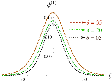
Figure 8: (Color online) Showing the variation of the positive potential K-dV solitons $\phi^{(1)}$ with the obliqueness of the wave propagation $\delta$ for $\alpha_{p}>\alpha_{pc}$ and for $\gamma=4/3$. The other plasma parameters are kept fixed.

To observe the influence of different plasma parameters on the propagation of solitary waves in magnetized quantum plasma, we derive the solution of K-dV equation (17). The stationary solitary wave solution of standard K-dV equation is obtained by considering a frame $\xi=\eta-u_{0}T$ (moving with speed $u_{0}$) and the solution is,

$${\rm\phi^{(1)}}=\rm\phi_{m}{\rm[sech^{2}}(\frac{\xi}{\Delta})],$$ (20)

where the amplitude, $\phi_{m}=3u_{0}/\lambda$, and the width, $\Delta=(4\beta/u_{0})^{1/2}$

IV MK-dV Equation

To obtain the MK-dV equation, same stretched co-ordinates is applied as we used in K-dV equation in section III (i.e., Eqs.(6) and (7)) and also used the dependent variables which is expanded as

$$n_{s}=1+\epsilon^{1/2}n_{s}^{(1)}+\epsilon n_{s}^{(2)}+\epsilon^{3/2}n_{s}^{(3)}+\cdot\cdot\cdot,$$ (21)

$$u_{ix,y}=0+\epsilon u_{ix,y}^{(1)}+\epsilon^{3/2}u_{ix,y}^{(2)}+\epsilon^{2}u_{ix,y}^{(3)}+\cdot\cdot\cdot,$$ (22)

$$u_{iz}=0+\epsilon^{1/2}u_{iz}^{(1)}+\epsilon u_{iz}^{(2)}+\epsilon^{3/2}u_{iz}^{(3)}+\cdot\cdot\cdot,$$ (23)

$$\phi=0+\epsilon^{1/2}\phi^{(1)}+\epsilon\phi^{(2)}+\epsilon^{3/2}\phi^{(3)}+\cdot\cdot\cdot,$$ (24)

we find the same expressions of $n_{i}^{(1)}$, $n_{e}^{(1)}$, $n_{p}^{(1)}$, $u_{iz}^{(1)}$, $u_{ix,y}^{(1)}$, $u_{ix,y}^{(2)}$ and $V_{p}$ by using the values of $\eta$ and $T$ in Eqs.(1)-(5) and (21)-(24) as before in section III. The next higher order series of $\epsilon$ of continuity, momentum and poisson’s equations as

$$\frac{\partial n_{i}^{(1)}}{\partial T}-V_{p}\frac{\partial n_{i}^{(3)}}{\partial\eta}+L_{x}\frac{\partial u_{ix}^{(2)}}{\partial\eta}+L_{x}\frac{\partial}{\partial\eta}(n_{i}^{(1)}u_{ix}^{(1)})$$

$$+L_{y}\frac{\partial u_{iy}^{(2)}}{\partial\eta}+L_{y}\frac{\partial}{\partial\eta}(n_{i}^{(1)}u_{iy}^{(1)})+L_{z}\frac{\partial u_{iz}^{(3)}}{\partial\eta}$$

$$+L_{z}\frac{\partial}{\partial\eta}(n_{i}^{(1)}u_{iz}^{(2)})+L_{z}\frac{\partial}{\partial\eta}(n_{i}^{(2)}u_{iz}^{(1)})=0,$$ (25)

$$\frac{\partial u_{iz}^{(1)}}{\partial T}-V_{p}\frac{\partial u_{iz}^{(3)}}{\partial\eta}+L_{z}\frac{\partial}{\partial\eta}(u_{iz}^{(1)}u_{iz}^{(2)})+L_{z}\frac{\partial\phi^{(3)}}{\partial\eta}=0,$$ (26)

$$L_{z}\frac{\partial\phi^{(3)}}{\partial\eta}-K_{11}L_{z}\frac{\partial n_{e}^{(3)}}{\partial\eta}-F\frac{\partial}{\partial\eta}(n_{e}^{(1)}n_{e}^{(2)})=0,$$ (27)

$$L_{z}\frac{\partial\phi^{(3)}}{\partial\eta}-K_{22}L_{z}\frac{\partial n_{p}^{(3)}}{\partial\eta}-G\frac{\partial}{\partial\eta}(n_{p}^{(1)}n_{p}^{(2)})=0,$$ (28)

$$\frac{\partial^{2}\phi^{(1)}}{\partial\eta^{2}}=\alpha_{e}n_{e}^{(3)}-n_{i}^{(3)}-\alpha_{p}n_{p}^{(3)},$$ (29)

where $F=K_{11}L_{z}(\gamma-2)$ and $G=K_{22}L_{z}(\gamma-2)$.

Now combining these higher order equations together with Eqs.(25)-(29) one can obtain

$$\frac{\partial\phi^{(1)}}{\partial T}+M\phi^{(1)2}\frac{\partial\phi^{(1)}}{\partial\eta}+N\frac{\partial^{3}\phi^{(1)}}{\partial\eta^{3}}=0.$$ (30)

This is well-known MK-dV equation that describes the obliquely propagating NA waves in a magnetized quantum plasma. where $M$ and $N$ are given by

$$M=\frac{V_{p}^{3}}{2L_{z}^{2}}\left[\frac{(\gamma-2)^{2}\alpha_{p}}{9K_{22}^{3}}-\frac{(\gamma-2)^{2}\alpha_{e}}{9K_{11}^{3}}+\frac{5L_{z}^{6}}{6V_{p}^{6}}\right],$$ (31)

$$N=\frac{V_{p}^{3}}{2L_{z}^{2}}\left[1+\frac{(1-L_{z}^{2})}{\omega_{ci}^{2}}\right].$$ (32)

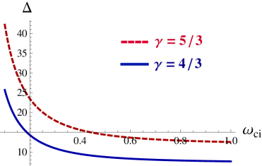
Figure 9: (Color online) Variation of $\Delta$ on solitary profile for different values of $\omega_{ci}$ when electron and positron being non-relativistic and ultra-relativistic degenerate.

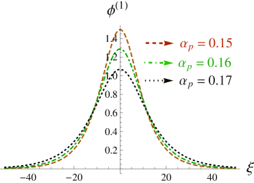
Figure 10: (Color online) Showing the variation of the amplitude of magnetized MK-dV solitons with $\alpha_{p}$ for $\alpha_{p}>\alpha_{pc}$ (in case of non-relativistic degenerate). The other plasma parameters are kept fixed.

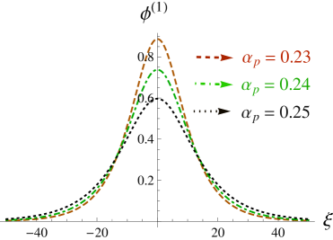
Figure 11: (Color online) Showing the variation of the amplitude of magnetized MK-dV solitons with $\alpha_{p}$ for $\alpha_{p}>\alpha_{pc}$ (in case of ultra-relativistic degenerate). The other plasma parameters are kept fixed.

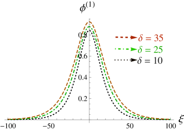
Figure 12: (Color online) Showing the variation of the amplitude of magnetized MK-dV solitons with $\delta$ for $\alpha_{p}>\alpha_{pc}$ (in case of non-relativistic degenerate). The other plasma parameters are kept fixed.

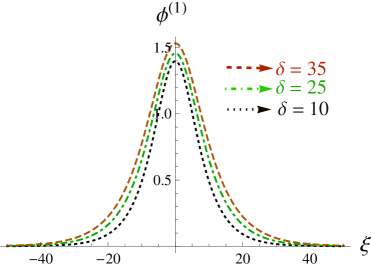
Figure 13: (Color online) Showing the variation of the amplitude of magnetized MK-dV solitons with $\delta$ for $\alpha_{p}>\alpha_{pc}$ (in case of ultra-relativistic degenerate). The other plasma parameters are kept fixed.

The stationary solitary wave solution of standard MK-dV equation is obtained by considering a frame $\xi=\eta-u_{0}T$ (moving with speed $u_{0}$) and the solution is,

$${\rm\phi^{(1)}}=\rm\phi_{m}{\rm[sech}(\frac{\xi}{\varpi})],$$ (33)

where the amplitude, $\phi_{m}=\sqrt{(6u_{0}/M)}$ and the width $\varpi={\sqrt{(N/u_{0})}}$.

V SG Equation

To drive the SG equation for NA SWs, we utitize the second order equation of surface charge density $\rho$ by analyzing Eqs. (1)-(5) and solution of which provides $\lambda=0$ since $\phi^{(1)}=0$. It is noted that at $\lambda=0$ its critical value $\alpha_{p}=\alpha_{pc}$. For $\alpha_{p}$ around its critical values $(\alpha_{pc})$, $\lambda=\lambda_{0}$ can be expressed as

$$\lambda_{0}\simeq s\left(\frac{\partial\lambda}{\partial\alpha_{p}}\right)_{\alpha_{p}=\alpha_{pc}}|\alpha_{p}-\alpha_{pc}|=sC_{1}\epsilon^{1/2},$$ (34)

where $|\alpha_{p}-\alpha_{pc}|$ is a small and dimensionless parameter, and can be taken as the expansion parameter $\epsilon^{1/2}$, i.e. $|\alpha_{p}-\alpha_{pc}|\simeq\epsilon^{1/2}$, and $s=1$ for $\alpha_{p}<\alpha_{pc}$ and $s=-1$ for $\alpha_{p}>\alpha_{pc}$. $C_{1}$ is a constant which is given by

$$C_{1}=-\frac{(\gamma-2)}{K_{22}^{2}}.$$ (35)

The surface charge density $\rho^{(2)}$ can be expressed as

$$\epsilon\rho^{(2)}\simeq-\frac{1}{2}\epsilon^{3/2}C_{1}s({\phi^{(1)}})^{2},$$ (36)

which, therefore, must be included in the third order Poisson’s equation. To the next higher order in $\epsilon^{3/2}$, we obtain the following equation

$$\frac{\partial^{2}\phi^{(1)}}{\partial\eta^{2}}+\frac{1}{2}sC_{1}({\phi^{(1)}})^{2}-\alpha_{e}n_{e}^{(3)}+n_{e}^{(3)}$$

$$+\alpha_{p}[\frac{1}{K_{22}}\frac{\partial\phi^{(3)}}{\partial\eta}-\frac{(\gamma-2)}{K_{22}^{2}}\frac{\partial}{\partial\eta}(\phi^{(1)}\phi^{(2)})$$

$$+\frac{(\gamma-2)^{2}}{3K_{22}^{2}}\frac{\partial(\phi^{(1)})^{3}}{\partial\eta}]=0.$$ (37)

After simplification, we can write from Eq. (37)

$$\frac{\partial\phi^{(1)}}{\partial T}+sC_{1}\alpha\phi^{(1)}\frac{\partial\phi^{(1)}}{\partial\eta}+\alpha\beta({\phi^{(1)}})^{2}\frac{\partial\phi^{(1)}}{\partial\eta}$$ (38)

$$+\alpha\gamma\frac{\partial^{3}\phi^{(1)}}{\partial\eta^{3}}=0.$$

Equation (38) is known as SG equation. It supports both the SWs and DLs solutions since it contains both $\phi$-term of K-dV and $\phi^{2}$-term of mK-dV equation. The Gardner equation derived here is valid for $\alpha_{p}\simeq\alpha_{pc}$.

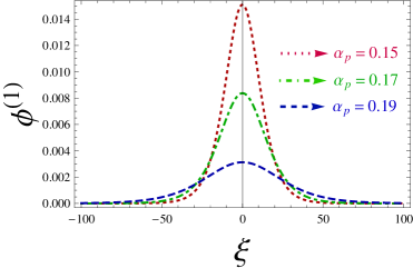
Figure 14: (Color online) Showing the variation of the amplitude of positive magnetized SGs solitons with $\alpha_{p}$ for $\alpha_{p}>\alpha_{pc}$ (in case of non-relativistic degenerate). The other plasma parameters are kept fixed.

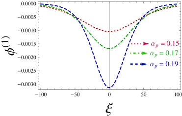
Figure 15: (Color online) Showing the variation of the amplitude of negative magnetized SGs solitons with $\alpha_{p}$ for $\alpha_{p}>\alpha_{pc}$ (in case of non-relativistic degenerate). The other plasma parameters are kept fixed.

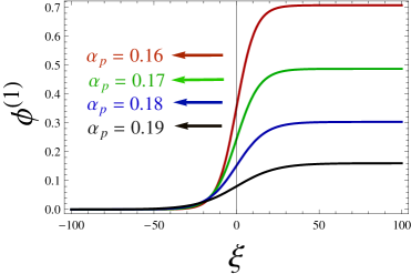
Figure 16: (Color online) Showing the variation positive potential DLs solitons with $\alpha_{p}$ in case of non-relativistic degenerate. The other plasma parameters are kept fixed.

By applying different boundary conditions in Eq. (38) one can find two type of solutions, namely solitary wave solution and double layer solution which are common in plasma literature Mannan2012 ; Alam2014 .

The SW solution of SG equation is given by the following equation:

$$\phi^{(1)}=\left[\frac{1}{\phi_{m2}}-\left(\frac{1}{\phi_{m2}}-\frac{1}{\phi_{m1}}\right)\cosh^{2}\left(\frac{\xi}{\Lambda}\right)\right]^{-1},$$ (39)

where

$$\phi_{m1,2}=\phi_{m}\left[1\mp\sqrt{1+\frac{U_{0}}{V_{0}}}\right],$$ (40)

$$U_{0}=\frac{C_{1}s\alpha}{3}\phi_{m1,2}+\frac{\alpha\beta}{6}\phi^{2}_{m1,2},$$ (41)

$$V_{0}=\frac{C_{1}^{2}s^{2}\alpha}{6\beta},$$ (42)

$$\phi_{m}=\frac{-C_{1}s}{\alpha},$$ (43)

$$\Lambda=\frac{2}{\sqrt{-\gamma\phi_{m1}\phi_{m2}}},$$ (44)

$$\gamma=\frac{\beta}{6}.$$ (45)

The DL solution of Eq. (38) is given by

$$\phi^{(1)}=\frac{\phi_{m}}{2}\left[1+\tanh\left(\frac{\xi}{\Lambda}\right)\right],$$ (46)

with

$$U_{0}=-\frac{s^{2}\alpha}{6\beta},$$ (47)

$$\phi_{m}=\frac{6U_{0}}{s\alpha},$$ (48)

$$\Lambda=\frac{2}{\phi_{m}\sqrt{-\gamma}},$$ (49)

where $\gamma=\beta/6$ and $\phi_{m}$ ($\Lambda$) is the DL height (thickness).

VI Discussions

We considered a relativistic magnetized four component EPI plasma system containing non-degenerate inertial light nuclei, both non-relativistically and ultra-relativistically degenerate electrons and positrons, and immobile heavy nuclei. The well-known reductive perturbation method has been used to drive the K-dV equation, and then solve it to examine an exact analytical expression for small amplitude solitary waves. In order to trace the effect of higher order nonlinearity, the mK-dV and SG equations have been derived since K-dV equation is valid only for the limits $\lambda\neq 0$, $\lambda>0$ and $\lambda<0$. By using this method, the K-dV, MK-dV and Gardner equations for NA SWs for ultradensed magnetized EPI plasmas are obtained and numerically analyzed the different plasma parameters. We have observed and analyzed that both compressive and rarefactive solitary waves (SWs) could exist for K-dV and GSs, but only rarefactive structures can be formed for MK-dV and DLs structures. We have observed K-dV solitons of both positive (Figs 3, 4, 7 and 8) and negative (Figs 5 and 6) potentials but that of positive (Figs 10, 11, 12 and 13 ) only for MK-dV solitons. On proceeding to more higher order calculation, we obtained Gardner equation as well as its solution, and from the GSs shown in Figs 14 and 15, we have investigated that both positive and negative potential GSs can be observed in the system. Further, we have studied and analyzed the DLs solution, and observed that only positive potential DL structure (Fig 16) can be found in the system. The plasma system under consideration supports finite amplitude solitary, gardner and double layer structures and their solutions are stable. The amplitude of SWs, GSs and DLs has been modified by the effect of degenerate pressure of electrons and positrons, this degenerate pressure is illustrated from the non-relativistic $({P_{e}}\propto{n_{e}}^{5/3})$ to ultra-relativistic $({P_{e}}\propto{n_{e}}^{4/3})$ regime. By using Chandrasekhar’s equation of state for relativistically degenerate electrons and positrons, it is examined that the relativistic factor greatly affects the speed of NA SWs where for the non-relativistic degenerate electrons and positrons, $\gamma=\frac{5}{3}$ and for the ultra-relativistic degenerate electrons and positrons, $\gamma=\frac{4}{3}$, and thus found that the relativistic factor, $\gamma=5/3~{}(non-relativistic)>\gamma=4/3~{}(ultra-relativistic)$ in every cases. In all cases, it is noticed that the relativistic corrections decrease the wave frequency, which, in the ultra-relativistic limit is smaller than the corresponding non-relativistic limit. The numerical results that have been found from our investigation are plotted in Figs. 1 - 16 and can be summarized as follows:

1. The four component EPI plasma system under consideration supports finite amplitude NA SWs, whose fundamental features (viz., amplitude, speed, and width) strongly depend on different plasma parameters, particularly, positron to ion number density ratio $\alpha_{p}$, obliqueness, cyclotron frequency $\omega_{ci}$, and the relativistic factor (i.e., non-relativistic limit and ultra-relativistic limit). We have numerically obtained here that for $\lambda=0$, the amplitude of the K-dV solitons become infinitely large, and the K-dV solution is no longer valid at $\lambda\simeq 0$. It has been observed that the solution of the K-dV equation supports both compressive (positive) and rarefactive (negative) structures depending on the critical value of $\alpha_{p}$.

2. In our present investigation, we have found that for $\alpha_{pc}=0.148$, the amplitude of the SWs breaks down due to the vanishing of the nonlinear coefficient $\lambda$. We have observed that at $\alpha_{p}>0.148$, positive (compressive) potential SWs exist, whereas at $\alpha_{p}<0.148$, negative (rarefactive) SWs exist (shown in Figs. 3-8).

3. It is found that the phase speed of the NA SWs decreases with the increasing values of electron to light nuclei number density ratio $\alpha_{e}$ and increases as the increasing values of positron to light nuclei number density ratio $\alpha_{p}$. The phase speed is always higher for the non-relativistic case than the ultra-relativistic case shown in Figs. 1 and 2.

4. It is shown that with the increase of $\alpha_{p}$, the amplitude and width of solitons waning gradually for positive potential, while the width of the solitons swelling gradually for negative potential. It is also seen that for non-relativistic limit the amplitude of the solitary waves is found to be greater than the ultra-relativistic limit shown in Figs. 3,4,5 and 6.

5. The variation of the amplitude of NA SWs is taken place with the different values of obliqueness of the wave propagation. It is observed that with the increase in obliqueness of the wave propagation, there is a increase in amplitude of the magnetized K-dV solitons which is exhibited in Figs. 7 and 8. It is noticed that as the value of $\delta$ increases, the amplitude of the solitary waves increases, while their width increases for the lower range of $\delta$ (from $0^{\circ}$ to about $50^{\circ}$), and decreases for its higher range (from $50^{\circ}$ to about $90^{\circ}$). We note that as $\delta\rightarrow 90^{\circ}$, the width goes to $0$, and the amplitude goes to $\infty$. This means that in case of larger values of $\delta$, the wave amplitude becomes large enough to break down the validity of the reductive perturbation method Alinejad2012 . Our present investigation is only valid for small value of $\delta$ but invalid for arbitrarily large value of $\delta$. The results that we have investigated in our present investigation support the results of Haider et al. Haider2012a ; Haider2012b .

6. Figure 9 shows that the width of the K-dV solitary profiles decrease with the increasing values of $\omega_{ci}$ for both non-relativistic and ultra-relativistic case. The solitary waves is also found to be greater for non-relativistic case than the ultra-relativistic case.

7. For MK-dV solitons, only compressive solitons are obtained, which is common in literature Rahman2014 . It is observed that the apmlitude of MK-dV solitons decreases with the increasing of $\alpha_{p}$ like as K-dV soliton as shown in Fig. 10 for non-relativistic limit and Fig. 11 for ultra-relativistic limit.

8. The amplitude of the magnetized MK-dV solitons affects notably by the obliqueness effect. From Figs. 12 and 13, we found that the amplitude of MK-dV solitons increases with the increasing of obliqueness.

9. In case of GSs, both the positive and negative structures are formed. It is investigated that like K-dV and MK-dV soliton the amplitude of magnetized GSs are decreases with the increasing of $\alpha_{p}$ as shown in Fig. 14 for positive potential and Fig. 15 for negative potential in non-relativistic limit.

10. It is observed that only positive potential DLs are exist. The amplitude of positive potential DLs decrease with the increasing of $\alpha_{p}$ as shown in Fig. 16.

We note that we have investigated obliquely propagating one-dimensional solitary structures by deriving the K-dV and MK-dV equations. However, one can derive Zakarov-Kuznetsove (ZK) equation to study multi-dimensional solitary structures and their multi-dimensional instability Mamun1988 , which is beyond the scope of our present work. It emphasizes here that the findings of our present investigation should be useful for understanding the basic features of the obliquely propagating NA SWs in ultra-relativistic degenerate magnetized plasmas which occur in many astrophysical compact objects, like white dwarfs, neutron stars, magnetars, etc.

VII Acknowledgments

B. Hosen, M. G. Shah and M. R. Hossen would like to thank Ministry of Science and Technology (MOST), Government of Bangladesh, for awarding the National Science and Technology (NST) fellowship.

References

- (1) W. Misner, K. S. Thorne, and J. I. Wheeler, Gravitation (Freeman, San Francisco, 1973).
- (2) M. C. Begelman, R. D. Blanford, and M. J. Rees, Rev. Mod. Phys. 56, 255 (1992).
- (3) H. R. Miller and P. J. Wiita, Active galactic nuclei (Springer, Berlin, 1987).
- (4) M. Tribeche, K. Aoutou, S. Younsi, and R. Amour, Phys. Plasmas 16, 072103 (2009).
- (5) E. P. Liang, S. C. Wilks, and M. Tabak, Phys. Rev. Lett. 81, 4887 (1998).
- (6) F. C. Michel, Rev. Mod. Phys. 54, 1 (1982).
- (7) M. R. Hossen and A. A. Mamun, Braz. J. Phys. 44, 673 (2014).
- (8) M. R. Hossen, S. A. Ema, and A. A. Mamun, Commun. Theor. Phys. 62, 888 (2014).
- (9) F. C. Michel, Theory of Neutron Star Magnetosphere (Chicago University Press, Chicago, 1991).
- (10) P. Goldreich and W. H. Julian, Astrophys. J. 157, 869 (1969).
- (11) E. Tandberg-Hansen and A. G. Emslie, The Physics of Solar Flares (Cambridge University Press, Cambridge, 1988).
- (12) M. J. Rees, Nature 229, 312 (1971).
- (13) M. L. Burns, A. K. Harding, and R. Ramaty, Positron-electron pairs in astrophysics (American Institute of Physics, Melville, New York, 1983).
- (14) S. I. Popel, S. V. Vladimirov, and P. K. Shukla, Phys. Plasmas 2, 716 (1995).
- (15) E. Tandberg-Hansen and A. G. Emshie, The Physics of Solar Flares (Cambridge University Press, Cambridge, 1988).
- (16) T. Piran, Phys. Rep. 314, 575 (1999).
- (17) W. H. Matthaeus, S. Dasso, J. M. Weygand, L. J. Milano, C. W. Smith, and M. G. Kivelson, Phys. Rev. Lett. 95, 231101 (2005).
- (18) N. Jehan, M. Salahuddin, H. Saleem, and A. M. Mieza, Phys. Plasmas 15, 092301 (2008).
- (19) A. S. Bains, A. P. Misra, N. S. Saini, and T. S. Gill, Phys. Plasmas 17, 012103 (2010).
- (20) S. Mahmood, A. Mushtaq, and H. Saleem, New J. Phys. 5, 28 (2003).
- (21) R. Sabry, W. M. Moslem, and P. K. Shukla, Phys. Plasmas 19, 122903 (2012).
- (22) N. Roy, M. S. Zobaer, and A. A. Mamun, J. Mod. Phys. 3, 850 (2012).
- (23) T. Akhter, M. M. Hossain, A. A. Mamun, Commun. Theor. Phys. 59, 745 (2013).
- (24) M. R. Hossen, L. Nahar, S. Sultana, and A. A. Mamun, Astro. Phys. Space Sci. 353, 123 (2014).
- (25) M. R. Hossen and A. A. Mamun, J. Korean Phys. Soc. 65, 2045 (2014).
- (26) S. L. Shapiro and A. A. Teukolsky, Black Holes, White Dwarfs, and Neutron Stars (John Wiley and Sons, New York, 1983).
- (27) A. A. Mamun and P. K. Shukla, Phys. Plasmas 17, 104504 (2010).
- (28) A. A. Mamun and P. K. Shukla, Phys. Lett. A 324, 4238 (2010).
- (29) M. Marklund and P. K. Shukla, Rev. Mod. Phys. 78, 591 (2006).
- (30) G. A. Mourou, T. Tajima, and S. V. Bulanov, Rev. Mod. Phys. 78, 309 (2006).
- (31) D. Koester and G. Chanmugam, Rep. Prog. Phys. 53, 837 (1990).
- (32) M. Azam and M. Sami, Phys. Rev. D 72, 024024 (2005).
- (33) S. Chandrasekhar, Philos. Mag. 11, 592 (1931).
- (34) S. Chandrasekhar, Mon. Not. R. Astron. Soc. 170, 405 (1935).
- (35) W. F. El-Taibany and A. A. Mamun, Phys. Rev. E 85, 026406 (2012).
- (36) H. R. Pakzad and K. Javidan, Astrophys. Space Sci. 331, 175 (2011).
- (37) Yin Ting and Wang, Way-Seen, IEEE Trans. Plasma Sci. 20, 419-424 (1992).
- (38) P. Chatterjee, D. K. Ghosh, and B. Sahu, Astrophys. Space Sci. 339, 261 (2012).
- (39) W. M. Moslem, I. Kourakis, P. K. Shukla, and R. Schlickeiser, Phys. Plasmas 14, 102901 (2007).
- (40) Q. Haque and H. Saleem, Phys. Plasmas 10, 2793-5 (2003).
- (41) W. Masood and A. Mushtaq, Phys. Lett. A 372, 4283 (2008).
- (42) F. B. Rizzato, Phys. J. Plasma Phys. 40, 289 (1988).
- (43) M. G. Shah, M. R. Hossen, and A. A. Mamun, Braz. J. Phys. 45, 219 (2015).
- (44) M. G. Shah, A. A. Mamun, and M. R. Hossen, J. Korean Phys. Soc. 66, 1239 (2015).
- (45) M. G. Shah, M. R. Hossen, and A. A. Mamun, J. Plasma Phys. 81, 905810517 (2015).
- (46) M. G. Shah, M. R. Hossen, S. Sultana, and A. A. Mamun, Chin. Phys. Lett. 32, 085203 (2015).
- (47) S. T. Shuchy, A. Mannan, and A. A. Mamun, JETP Lett. 95, 310 31 (2012).
- (48) Y. Wang, Z. Zhou, Y. Lu, X. Ni, J. Shen, and Y. Zhang, Commu. Theor. Phys. 51, 1121 (2009).
- (49) S. K. El-Labany and S. M. Shaaban, J. Plasma Phys. 53, 245 (1995).
- (50) S. A. Khan, Phys. Plasmas 19, 014506 (2012).
- (51) I. Zeba, W. M. Moslem, and P. K. Shukla, Astrophys. J. 750, 72 (2012).
- (52) W. Masood, B. Eliasson, and P. K. Shukla, Phys. Rev. E 81, 066401 (2010).
- (53) M. R. Hossen, L. Nahar, S. Sultana, and A. A. Mamun, High Energy Density Phys. 13, 13 (2014).
- (54) M. R. Hossen and A. A. Mamun, Braz. J. Phys. 44, 673 (2014).
- (55) M. R. Hossen, L. Nahar, S. Sultana, and A. A. Mamun, Phys. Scr. 89, 105603 (2014).
- (56) M. R. Hossen and A. A. Mamun, Plasma Sci. Technol. 17, 177 (2015).
- (57) A. Mannan, and A. A. Mamun, Astrophys. Space. Sci. 340, 109 (2012).
- (58) M. S. Alam, M. M. Masud, and A. A. Mamun, Astrophys. Space. Sci. 349, 245 (2014).
- (59) H. Alinejad, Phys. Plasmas 19, 052302 (2012).
- (60) M. M. Haider, S. Akhter, S. S. Duha, and A. A. Mamun, Open Phys. 10, 1168 (2012).
- (61) M. M. Haider and A. A. Mamun, Open Phys. 19, 102105 (2012).
- (62) M. M. Rahman, M. S. Alam, and A. A. Mamun, Eur. Phys. J. Plus 129, 84 (2014).
- (63) A. A. Mamun, Phys. Scr. 58, 505 (1988).