GRAVITY spectro-interferometric study of the massive multiple stellar system HD 93 206 A

Abstract

Characterization of the dynamics of massive star systems and the astrophysical properties of the interacting components are a prerequisite for understanding their formation and evolution. Optical interferometry at milliarcsecond resolution is a key observing technique for resolving high-mass multiple compact systems. Here we report on VLTI/GRAVITY, Magellan/FIRE, and MPG2.2m/FEROS observations of the late-O/early-B type system HD 93 206 A, which is a member of the massive cluster Collinder 228 in the Carina nebula complex. With a total mass of about 90 M_⊙, it is one of the most compact massive-quadruple systems known. In addition to measuring the separation and position angle of the outer binary Aa - Ac, we observe Br$\gamma$ and HeI variability in phase with the orbital motion of the two inner binaries. From the differential phases ($\Delta_{\phi}$) analysis, we conclude that the Br$\gamma$ emission arises from the interaction regions within the components of the individual binaries, which is consistent with previous models for the X-ray emission of the system based on wind-wind interaction. With an average 3-$\sigma$ deviation of $\Delta_{\phi}\sim$15^∘, we establish an upper limit of p$\sim$0.157 mas (0.35 AU) for the size of the Br$\gamma$ line-emitting region. Future interferometric observations with GRAVITY using the 8m UTs will allow us to constrain the line-emitting regions down to angular sizes of 20 $\mu$as (0.05 AU at the distance of the Carina nebula).

1 Introduction

One of the most important observational clues to understand the formation of massive stars is multiplicity (see e.g., Apai et al., 2007; Zinnecker & Yorke, 2007; Peter et al., 2012; Chini et al., 2012). Some plausible mechanisms to form massive multiples include: (a) disk fragmentation (Bonnell & Bastien, 1992; Monin et al., 2007; Krumholz et al., 2009); (b) the accretion of wider low-mass systems (Bonnell & Bate, 2005; Maeder & Behrend, 2002); (c) formation through failed mergers and stellar collisions in early dynamical interactions (Zinnecker & Bate, 2002) and; (d) disk-assisted capture (Bally & Zinnecker, 2005). To discern which of the aforementioned models should be preferred, an analysis of the orbital properties in multiple systems (e.g., period distribution, mass ratios, orbital eccentricities, coplanarity, etc) is required. This is not an easy task, because companions can cover spatial scales from a few 1/10 Astronomical Units (AU) to 1000s of AU, and contrast ratios of components can span several orders of magnitudes.

Sana et al. (2014) conducted the first statistical survey of massive multiple systems combining observations with high angular resolution facilities (particularly optical interferometry) with archival spectroscopic data. With a main sample of 96 O-stars, this study indicates that $\sim$90% of the massive stars are at least binaries and that $\sim$30% of them belong to a higher-degree multiple system. For example, the Trapezium system in Orion (Weigelt et al., 1999; Schertl et al., 2003; Kraus et al., 2009) is one of these systems which reveals the existence of stellar companions at multiple spatial scales. In fact, all of its four main components, like $\theta$1 Ori B (Close et al., 2013), turn out to be embedded “micro-clusters” or binaries. However, it is not yet clear whether (i) these systems are stable on long time scales and; (ii) how dynamical interactions with the companions can affect their evolution. Allen (2015) suggested that quintuplet systems, like $\theta$1 Ori B, are prone to dissolve in around $\sim$100 crossing times, with some of the components merging or ejected (i.e., being the progenitors of runaway stars; see also Fujii & Portegies Zwart, 2011).

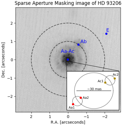
Figure 1: The image displays the Sparse Aperture Masking image of the system HD 93 206. The position of the components Aa-Ac, Ab and E are shown with a blue dot. The two concentric dashed rings encircle the central 2 and 4 arcseconds around HD 93 206 A. The inset shows the quadruple system Aa-Ac, which is the target of this work. The image was taken with VLT-NACO in the K_s-filter ($\lambda_{0}$ = 2.2 $\mu$m).

Therefore, resolving the components of high-degree multiple systems, both in a statistical way and targeting individual systems, and monitoring their orbital motions are mandatory to answer the aforementioned questions. For this purpose, several high-angular resolution techniques are required. Among them, infrared long-baseline interferometry is one of the most crucial techniques to characterize compact systems where the resolution provided by classical imaging techniques (e.g., speckle imaging or Adaptive Optics imaging) is limited. This is particularly true, now that the foremost $K-$band beam combiner GRAVITY has been successfully deployed at the Very Large Telescope Interferometer (VLTI). The new capabilities of GRAVITY, not only offer us the possibility to observe high-mass multiples with milliarcsecond resolution, but also at an intermediate spectral resolution (R$\sim$4000) and higher sensitivity than previous interferometric instruments. In this study, we present the results of a GRAVITY spectro-interferometric study of HD 93 206 A, an X-ray emitter that is known to be one of the most compact massive quadruple systems in the Galaxy. The object has been frequently investigated as a template for the formation of massive multiples.

Table 1: Observed stellar pairs in HD 93 206. Component nomenclature follows the WDS (see text). The rest of the information comes from the listed references.

Pair	Year	PA	sep.	$\Delta m$	Reference
		(deg)	(″)	(mag)
Aa,Ab	2014	324	1.00	3.9	Sana et al. (2014)
Aa,Ac	2016	328	0.03	0.4	This work
A,B	2012	276	7.07	5.8	Sana et al. (2014)
A,C	1934	93	8.80	—	Dawson & Aguilar (1937)
A,E	2012	303	2.58	7.2	Sana et al. (2014)

1.1 The source: HD 93 206 A

HD 93 206 ($\equiv$QZ Car) is a complex multiple system (see Fig. 1) that is the brightest member of the open cluster Collinder 228, located in the Carina Nebula at a distance of 2.3 $\pm$ 0.1 kpc (Walborn, 1995; Smith, 2002, 2006). The known resolved components are listed in Table 1. Before proceeding, some clarifications are in order:

• There is some confusion in the literature regarding component nomenclature. Here we follow the one of the Washington Visual Double Catalog (WDS, Mason et al., 2001), which is the one that deals with the parent-child relationships most accurately.

• In the current WDS classification, the components of Aa-Ac form a quadruple system of 2 spectroscopic binaries with Ac being an eclipsing binary. In contrast, the nomenclature of Sana et al. (2014) includes both spectroscopic binaries in component Aa, and defines each member with numbers from 1 to 4.

• Component E identified in the classification of Sana et al. (2014) corresponds to component D in the WDS.

• Component C could be a spurious detection. It has not been observed since 1934, and it is not detected as a 2MASS source.

• Components Ab, B, and D (and C if it is real) are significantly dimmer ($\Delta_{m}>$3.0 mag) than Aa and Ac, which dominate the light output of the system and are the only ones bright enough to contribute to the integrated spectrum.

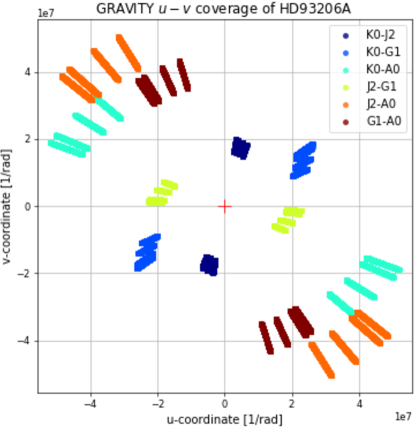
Figure 2: GRAVITY/VLTI $u-v$ coverage of HD 93 206 A obtained during the Science Verification run of the instrument. Four snapshots per baseline were recorded. Baselines are indicated with different colors.The red cross indicates the center of the $u-v$ plane.

This paper deals with the two bright central binaries Aa and Ac (see Fig 1). Speckle observations with the CHARA speckle camera (Mason et al., 1998) and direct imaging with the Fine Guidance Sensor of the Hubble Space Telescope (Nelan et al., 2004) could not resolve Aa-Ac, setting an upper limit of $\rho\sim$15.2 mas ($\sim$35 AU) for their separation. However, $H$-band interferometric data taken with PIONIER (Precision Integrated-Optics Near-infrared Imaging ExpeRiment) at the Very Large Telescope Interferometer (VLTI) and $K$-band sparse aperture masking (SAM) observations obtained with the near-infrared camera NACO at the Very Large Telescope (VLT) resolved the separation between the two binaries Aa and Ac, finding a projected angular distance of $\rho\sim$26 mas (64.4 AU in projection) and with brightness ratios of $\Delta H=0.42$ mag and $\Delta K_{\rm S}=1.18$ mag (Sana et al., 2014).

The spectroscopic analysis of the system (Leung et al., 1979; Morrison & Conti, 1980; Stickland & Lloyd, 2000; Mayer et al., 2001) indicates the existence of two periods of 20.7 d and 6 d for components Aa and Ac, respectively. Therefore, from the spectroscopic point of view, HD 93 206 Aa-Ac is a quadruple system that can be subdivided into two short-period binary systems, Aa1,Aa2 and Ac1,Ac2, in a long-period orbit of $\sim$50 years around each other. This configuration is different to other hierarchical quadruple systems (such as HD 17 505 Hillwig et al., 2006; Sota et al., 2011) composed of four O-stars in which components are organized in a close pair (with period of days) orbiting a third star with a period of years and a fourth star orbiting around the other three with a period possibly measured in millennia. The intriguing architecture of the system highlights the importance of characterizing the orbital motion of the components in HD 93 206 A with the final goal to confront the different formation scenarios with its dynamical properties. For example, Core Collapse massive star formation models (e.g., Krumholz et al., 2009) assume that companions have coplanar orbital planes, while competitive accretion models (e.g., Bonnell & Bate, 2006) predicts non-coplanar orbits.

The spectroscopic analysis also suggests that Ac1,Ac2 is in fact a semi-detached eclipsing binary, and Aa1,Aa2 is identified as a long-period spectroscopic binary. The individual spectral classification of the stellar components in HD 93 206 Aa-Ac supports that Aa1 is an O-type supergiant with a spectral type O9.7 Iab or O9.5 I (the classification for the combined spectral type is O9.7 Ibn, Sota et al. 2014). Aa2 is undetected in the spectrum but indirect evidence points towards it being several times less massive than Aa1 and with a spectral type in the vicinity of B2 V. Ac1 appears to be a giant or supergiant (O8 III or B0 Ib). Although the primary Ac1 is the brightest component, it seems to be less massive than the secondary Ac2 (possibly O9 V, but its signature on the integrated spectrum is weak), which suggests a case-B mass transfer within this binary. The whole system has an estimated total mass of $\sim$90 M_⊙ (Leung et al., 1979; Morrison & Conti, 1980; Mayer et al., 2001).

X-ray observations of the quadruple Aa-Ac (Townsley et al., 2011; Broos et al., 2011) revealed an excess in X-ray emission (average $\sim$7x10^-13 erg  s^-1cm^-2) over the expected cumulative bolometric luminosity. A three component plasma model fitted to the observed X-ray spectra by Parkin et al. (2011) supports the presence of shock heated plasma from wind-wind collision shocks. Those authors suggest that the system Ac is the main X-ray emitter. However, the total observed X-ray flux might be the sum of the emission of the individual components and the mutual wind-wind collision region between the two binaries. If this hypothesis is correct, we expect to observe infrared shock tracers (like Br$\gamma$) to be formed in an extended region where the colliding winds of the two binary systems interact.

The paper is outlined as follows: Sec. 2 presents our GRAVITY/VLTI observations and data reduction. In Sec. 3 the analysis of the interferometric observables and of the source spectrum are described. In Sec. 4 our results are discussed and, finally, in Sec. 5 the conclusions are presented.

2 Observations and data reduction

2.1 GRAVITY observations

HD 93 206 A was observed for a total of two hours with GRAVITY (Eisenhauer et al., 2008, 2011; GRAVITY Collaboration et al., 2017) during the ESO Science Verification run of the instrument. Snapshot observations were obtained at four different hour angles, two of them during June 17th, 2016 and two more during June 18th, 2016. The observations were carried out using the highest spectral resolution (R$\sim$4000) of the interferometer in the $K-$band (1.990 $\mu$m – 2.450 $\mu$m), together with the combined polarization and single-field modes of the instrument. With this configuration, GRAVITY equally splits the incoming light of the science target between the fringe tracker and science beam combiners to produce interference fringes simultaneously in each one of them. While the science beam combiner disperses the light at the desired spectral resolution, the fringe tracker beam combiner always works with a low-spectral resolution of R$\sim$22 (Gillessen et al., 2010) but at a high frequency sampling ($\sim$1 kHz). This allows to correct for the atmospheric piston, stabilizing the fringes of the science beam combiner for up to several tens of seconds.

Table 2: GRAVITY/VLTI science target and calibrator data sets.

Date	Target	Typea	$K_{\mathrm{mag}}$	DITb	NDITc	No. PAd	Airmasse	Seeinge	UD sizef
17-06-2016	HIP 50 644	CAL	4.25	30	10	2	1.49, 1.54	0.45, 0.51	0.853
	HD 93 206 A	SCI	5.25	30	10	2	1.54, 1.67	0.57, 0.54	-
	HD 94 776g	CAL	3.40	10	26	2	1.73, 1.79	0.80, 0.65	0.917
	HD 149 835	CAL	4.90	30	10	2	1.17, 1.19	0.34, 0.64	0.49
	HD 188 385	CAL	5.99	30	10	2	1.45, 1.51	0.47, 0.43	0.224
18-06-2016	HD 93 206 A	SCI	5.25	30	10	2	1.40, 1.43	1.0, 0.77	-
	HD 94 776g	CAL	3.40	10	26	2	1.45, 1.47	0.57, 0.53	0.917
	HD 166 521	CAL	4.52	30	10	2	1.06, 1.07	0.48, 0.48	0.578
	HD 164 031	CAL	4.11	30	10	2	1.31, 1.37	0.59, 0.88	0.707
	HD 8315	CAL	4.04	30	10	1	1.18	0.78	0.749

• This parameter indicates the purpose of the target observed. CAL means that the source corresponds to a calibrator star and SCI means that the source corresponds to our science target.

• Detector integration time in seconds.

• Number of frames to estimate the complex visibilities per data cube.

• Number of observed position angles per night.

• Airmass and Seeing per target data set.

• $K-$band estimated Uniform Disk size in milliarcseconds obtained from SearchCal (Bonneau et al., 2006, 2011).

• K0III star used to calibrate the HD 93 206 A spectrum.

All the HD 93 206 A data were recorded with the A0-G1-J2-K0 configuration of the 1.8-meter Auxiliary Telescopes (ATs) of the VLTI. This configuration provides a maximum projected baseline of $\sim$120 meters (J2-A0) and a minimum one of $\sim$39 meters (K0-J2) for the target coordinates. These baseline lengths correspond to a maximum angular resolution ($\theta$=$\lambda$/2B) of $\theta\sim$1.89 mas and a minimum one of $\theta\sim$5.8 mas, at a central wavelength of $\lambda_{0}$= 2.2 $\mu$m. Figure 2 displays the science target $u-v$ coverage obtained with the aforementioned GRAVITY observations.

The interferometric observables (squared visibilities, closure phases, and differential phases) as well as the source’s spectrum were obtained using the version 0.8.4 of the instrument’s data reduction software provided by ESO (Lapeyrere et al., 2014); it uses of a series of esorex recipes to estimate the raw observables and calibrate them. The data reduction process converts the science camera frames (where the interference fringes are recorded using the ABCD sampling method, Colavita et al., 1999) into a set of 1D-spectra from which the observables are estimated.

First, the science detector is characterized by measuring its bias, pixel gain, bad pixel and wavelength maps. The wavelength maps of the Fringe Tracker and Science beam combiners are calibrated using the GRAVITY Calibration Unit (Blind et al., 2014). For the Science Beam Combiner, the fiber wavelength scale is obtained through observations of the internal Halogen lamp having the Fiber Differential Delay Lines in close-loop and fringe tracking. At the same time, the calibration unit delay line positions are modulated, while their position is monitored using the internal laser diode ($\lambda_{0}$ = 1.908 $\mu$m). The measured fringe phase shifts are converted to wavelength knowing the introduced OPD offsets, with a wavelength precision of $\Delta\lambda$ = 2nm. An Argon spectral calibration lamp (which provides 10 lines in the GRAVITY wavelength range) is used to derive the vacuum wavelength scale and correct the wavelength map of the fiber dispersion, achieving an absolute wavelength calibration equivalent to 1/2 of spectral element at the highest spectral resolution of the instrument (0.1 nm, equivalent to a relative uncertainty of $5\times 10^{-5}$ in high spectral resolution mode).

The transfer function of the science beam combiner is calibrated by using the P2VM algorithm (Tatulli et al., 2007; Lacour et al., 2008). It, first, requires to determine the V2PM matrix, as defined in Lapeyrere et al. (2014), for each spectral bin. The internal Halogen lights are used to calibrate this matrix in three steps: first, for the power transmission of each one of the telescopes; second, by computing the visibility amplitude and phase for each baseline (i.e., internal contrast and phase) produced by an induced optical path delay (OPD) modulation and; third, by computing the closure phases. Finally, the inverse of the V2PM matrix is used to extract the interferometric observables from on-sky observations. The P2VM calibration files are generated from the raw data with the esorex recipe gravity_p2vm. Once they are created, the gravity_vis recipe can be used to extract the total flux per telescope and correlated flux per baseline (i.e., the raw observables). The recipe gravity_vis includes a bootstrapping method to compute the complex visibility and bispectrum errors, as well as a visibility-loss correction factor due to the integration time difference between the fringe tracker frames and the science ones.

To calibrate the interferometric observables, interleaved observations of the science target and point-like sources were performed. Table 2 displays the observational setup used for the science target together with the different calibrators. The interferometric calibration was performed using the gravity_viscal recipe. This routine computes the instrumental transfer function by correcting the observed calibrator visibilities by the theoretical ones according to the estimated angular size of the calibrator. The algorithm then groups calibrators with the same observational setup as the science target and interpolates their transfer functions to the acquisition time of the science target observations. Finally, the recipe corrects the target raw visibilities for the estimated transfer function, delivering the calibrated observables.

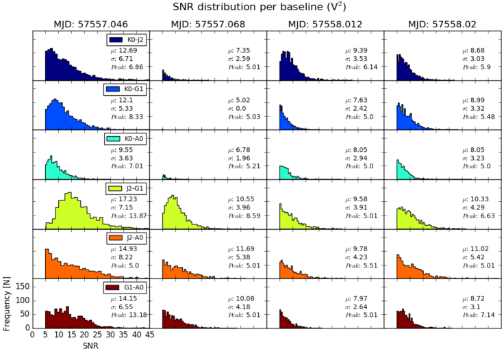
Figure 11: SNR distributions of the V². Every column in the plot corresponds to a different GRAVITY data set. Histograms for different baselines are plotted in different colors (see label on the figure). The values of the mean and standard deviation of the SNR, as well as of the peaks of the distributions are printed on each panel in the figure.

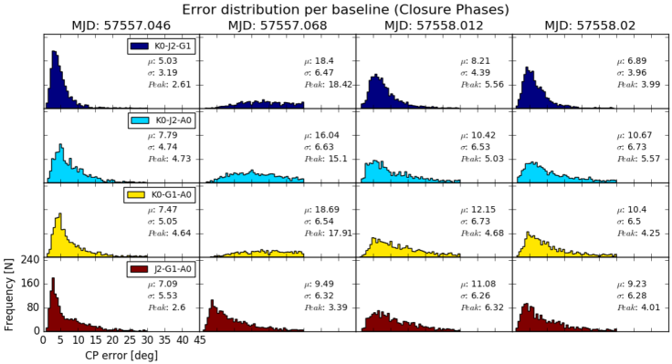
Figure 12: Closure phase error distributions. Every column in the plot corresponds to a different GRAVITY data set. Histograms for different baselines are plotted in different colors (see label on the figure). The values of the mean and standard deviation of the closure phase errors, as well as of the peaks of the distributions are printed on each panel in the figure.

Before analyzing the data, those V² points with a SNR $\leq$ 5 and closure phases with $\sigma_{cp}\geq$ 40^∘ were flagged. Figures 11 and 12 in the Appendix A display the distributions of the V² SNR and of the errors in the closure phases after flagging. From these distributions, it is observed that three baselines have a considerably small SNR, particularly in the second data set where only a few points remain after flagging. These baselines are connected with the K0 station, which shows a poor transmission throughput at the time of the Science Verification observations. The first data set has the highest quality mainly because of the excellent weather conditions under which it was taken (see Table 2).

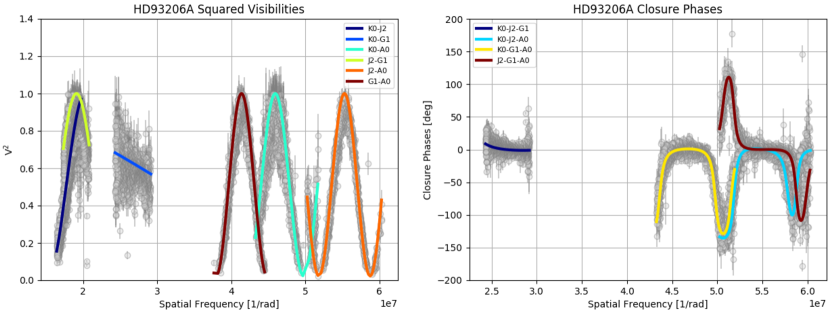
Figure 3: Calibrated V² visibilities and closure phases versus spatial frequency. One data set of the GRAVITY/VLTI observations is displayed with gray dots (MJD: 57557.046). The best-fit average model is overplotted with color lines. Baselines are indicated with different colors and their corresponding telescope stations displayed on the frames.

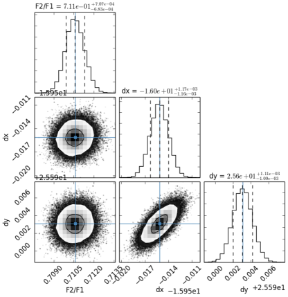
Figure 4: Posterior distributions of the fitted parameters. The 2D distributions shows 1 and 2 standard deviations encircled by a black contour. The position in the distributions of the best-fit solution found with the non-linear least squares method is displayed with a blue square. The 1D histograms show the expected value, $\mu$, and $\pm$1$\sigma$ with vertical dashed lines, together with their corresponding values at the top.

2.2 FIRE observations

In order to determine the K-band spectral features present in the HD 93 206 A spectrum, we have obtained near-infrared spectra using the Folded-port InfraRed Echellette (FIRE; Simcoe et al., 2013) spectrograph, attached to the 6.5 m Baade Magellan Telescope at Las Campanas Observatory. Observations were gathered on March 28th, 2016 (HJD 2457475.66). We have obtained four one second exposure at airmass 1.17, under excellent seeing conditions (0.5 arcsec). FIRE was used in echelle mode, and the selected slit width was 0.6 arcsec. The FIRE spectrum is spread over 21 orders from 0.82 to 2.51 microns, providing a resolving power R$\sim$6000. The star observations were followed by a bright telluric standard of spectral type A0V, in this case HD 83 280.

Data reduction and the spectral extraction were performed with the FIREHOSE package. It is based on the MASE (Bochanski et al., 2009) and SpeXtool packages (Vacca et al., 2003; Cushing et al., 2004). At the beginning of the night, we have also obtained dome flats and Xenon flash lamps to build a pixel-to-pixel response calibration. For wavelength calibration we used Thorium-Argon lamp exposures taken immediately after the target exposures, and OH sky emission lines extracted from the target exposures. The telluric correction was accomplished using the methods and routines developed in SpeXtools.

Adopting the ephemeris published by Mayer et al. (2001) for Aa-Ac, the FIRE spectrum of HD 93 206 A corresponds to phase 0.97 of the orbit of Ac, that is in the primary eclipse of the system Ac, and phase 0.74, which corresponds to the maximum radial velocity for the primary (Aa1) in the pair Aa. We should take into account that the errors reported in the ephemeris of both systems could lead to phase errors of about 3% for system Ac and 15% for system Aa.

2.3 FEROS observations

Optical spectroscopic results are presented in Section 4. The data were obtained as part of the OWN Survey (Barbá et al., 2010). They were gathered using the FEROS spectrograph attached to the 2.2 m MPG/ESO telescope at La Silla, in May 2-5th, 2009 and May 21th, 2012. These FEROS observations were reduced with the pipeline provided by ESO in the MIDAS environment.

3 Data analysis

3.1 Modeling the interferometric observables

3.1.1 MCMC modeling

In the calibrated V² and closure phases, the target presents the prototypical cosine signature of a resolved binary system. Figure 3 displays one of the GRAVITY data sets (MJD:57557.046) where the binary signature is clearly visible. As expected, with the current GRAVITY observations we could only map the separation between the two components Aa and Ac, but not resolve the individual components of these binaries (which have angular separations considerably less than 1 mas). A geometrical model fitting of a binary composed of two point-like sources was applied to the observables. The expression used to estimate the complex visibilities, $V\mathrm{(u,v)}$, is the following one:

$$V\mathrm{(u,v)}=\frac{1+\mathrm{F_{Ac}/F_{Aa}}G(\zeta)e^{-2\pi j\mathrm{(\Delta\theta_{x}u+\Delta\theta_{y}v)}}}{1+\mathrm{F_{Ac}/F_{Aa}}}\,,$$ (1)

with,

$$G(\zeta)=|\frac{sin\zeta}{\zeta}|\,\,\,\,\,\,\mathrm{with}\,\,\,\,\,\,\zeta=\frac{\pi\mathrm{(\Delta\theta_{x}u+\Delta\theta_{y}v)}}{R}\,,$$ (2)

where $\mathrm{F_{Ac}/F_{Aa}}$ is the flux ratio between the components of the binary, (u, v) are the components of the spatial frequency sampled per each observed visibility point (u=B_x/$\lambda$ and v=B_y/$\lambda$), and ($\Delta\theta_{x}$, $\Delta\theta_{y}$) are the East-West and North-South components of the projected angular separation between primary and secondary components of the binary. $G(\zeta)$ is a correction factor due to the bandwidth smearing of the finite bandpass used and R=$\lambda/\Delta\lambda$ is the spectral resolution of the interferometer (in this case R$\sim$4000). The total flux of the binary is normalized to unity such that F_Aa+F_Ac=1.

V² and closure phases across the entire bandpass were simultaneously used to estimate the average $\mathrm{F_{Ac}/F_{Aa}}$ and ($\Delta\theta_{x}$, $\Delta\theta_{y}$) of the binary. The fitting process was performed using a dedicated Markov chain Monte-Carlo (MCMC) routine based on the python software emcee (Foreman-Mackey et al., 2013). First, an approximation of the best-fit parameters was obtained using the non-linear least squares minimization algorithm inside the python library scipy.optimize. To account for the standard deviations and correlations of the model parameters, we explore the solution space around the best-fit values obtained with the least squares method; 300 random points with a linear distribution between $\pm$10$\sigma$ were generated for each one of the parameters. For every random point, 700 iterations were performed using the MCMC algorithm to maximize the posterior probability of the model. The $\chi^{2}$ of the best-fit model is $\chi^{2}=$ 3.93, while the parameter values and three-sigma uncertainties of the best-fit model are reported in Table 3. Figure 4 shows the posterior probability distributions of the parameters, their correlations, as well as their individual marginalized distributions in 1D histograms along the diagonal of the plot.

Table 3: Best-fit geometrical model with the different algorithms used in this work.

	MCMC fit		LitPro fit		CANDID fit		Average fit
Parameter	Value	$\pm 3\sigma$	Value	$\pm 3\sigma$	Value	$\pm 3\sigma$	Value	$\pm 3\sigma$
$\mathrm{F_{Ac}/F_{Aa}}$	0.710	$\pm$0.002	0.67	$\pm$0.11	0.832	$\pm$0.004	0.740	$\pm$0.14
$\Delta\theta_{x}$ [mas]	-15.965	$\pm$0.0013	-15.91	$\pm$0.020	-15.942	$\pm$0.0054	-15.940	$\pm$0.045
$\Delta\theta_{y}$ [mas]	25.593	$\pm$0.0034	25.645	$\pm$0.024	25.591	$\pm$0.005	25.609	$\pm$0.054

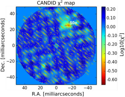
Figure 5: The figure displays the CANDID interpolated map of the $\chi^{2}$ in a field-of-view of 100 mas. The position of the secondary is marked with a red cross. The color scale is logarithmic. The yellow lines indicate the convergence vectors (from the starting points to the final fitted position) of the Levenberg-Marquardt algorithm for each one of the points sampled in the grid.

3.1.2 LitPro modeling

Additionally, to our MCMC modeling, we also performed the analysis of the binary using LitPro (Tallon-Bosc et al., 2008). This is a code that uses a gradient descent method to perform the optimization; it is based on a Levenberg-Marquardt algorithm combined with a Trust Region method. The software allowed us to use several pre-defined geometrical components to represent the interferometric data. In this case, we use a similar setup to the MCMC model (a binary composed of two point-like sources). There are two main differences between the two methods: (i) the first one is the lack of a correction in LitPro due to bandwidth smearing; (ii) the second one is the flagging method applied by LitPro, which masks $V^{2}<$ 3$\sigma_{V^{2}}$ or $V^{2}>$ 1+ 3$\sigma_{V^{2}}$ . Table 3 displays the best-fit model obtained with this software with an achieved $\chi^{2}$=3.89. Despite the differences in the algorithms and their setup, the parameters obtained with MCMC and LitPro are in very good agreement.

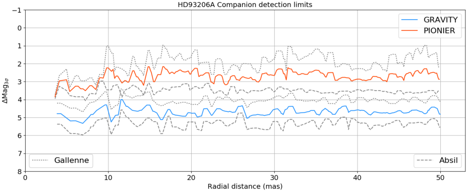
Figure 6: 3$\sigma$ contrast limits of secondary components are plotted for separations between 3 and 50 mas in the GRAVITY and PIONIER data of HD 93 206 A. The red and blue solid lines indicate the average detection limits between the two detection methods used. The response of each one of the detection algorithms is plotted in dotted and dashed gray lines for the Absil et al. (2011) and Gallenne et al. (2015) methods, respectively.

3.1.3 CANDID modeling and detection limits

We also used CANDID (Gallenne et al., 2015) to analyze the interferometric data of HD 93 206 A. This Python code uses an Levenberg-Marquardt algorithm to fit for a binary system performing a systematic exploration over a given grid. The model of the binary represents a spatially resolved primary component (to which a uniform disk is fitted), as well as the bandwidth smearing of the visibilities (see Lachaume & Berger, 2013). In this case, we considered the two components of the binary to be unresolved and the size of the binary component was set to zero. For the grid search, we selected a step of p=1.89 mas, which is equivalent to $\lambda$/2B_max. Additionally to the binary fitting, CANDID also allows to obtain an estimation of the 3$\sigma$ detection limit for companions at different separations from the primary. The code includes the algorithms described in Absil et al. (2011) and Gallenne et al. (2015) to look for high-contrast companions in the searched grid.

Table 3 displays the best-fit parameters obtained with CANDID. Figure 5 displays the map of the $\chi^{2}$ minima of the binary model with the position of the secondary marked with a red cross. In the case of our data, the secondary was detected with the highest confidence value allowed by CANDID (50$\sigma$). The minimum $\chi^{2}$ achieved by the searching algorithm is $\chi^{2}$ =2.46. The flux ratio and position of the secondary found with CANDID agrees with the values obtained with the other two methods previously described (see Table 3).

CANDID was also used to estimate the maximum 3$\sigma$ magnitude difference, $\Delta$Mag_3σ, to detect a companion for a separation range between 3 and 50 mas using both detection methods available in the code. Here, we only used one of the GRAVITY data sets (MJD:57557.046), to properly compare the results with the 2012 PIONIER data set reported by Sana et al. (2014). The published PIONIER astrometric position and flux ratio were adopted to subtract the secondary component from the data and search for faint companions in the grid with a step of p=1.4 mas. Figure 6 displays the resulting detection limits. The blue and red solid lines indicate the average detection limits between the two detection methods available in CANDID. These results support that the maximum detectable magnitude difference in the PIONIER data is $\sim$3 mag, while for GRAVITY it goes up to $\sim$5 mag.

As evident in Table 3, the model parameters obtained with the three different methods agree quite well. However, the standard deviation obtained for each of the algorithms appears to be underestimated. This is mainly caused by slight deviations in the used expressions for the optimization, as well as from the flagging methods applied in each one of the methods. To obtain a more robust estimation of the best-fit parameters and their uncertainties, we computed the mean and the standard deviation among the best-fit models determined with the different optimization methods. These estimates are also reported in columns 8 and 9 in Table 3, and those are the values adopted for the following analysis in this work. Figure 3 displays (for clarity) one of the GRAVITY data sets together with the best-fit average model overplotted. Notice how the trend in V² and CPs are well reproduced by the best-fit model.

3.2 Extracting the source spectrum

Together with the interferometric observables, GRAVITY delivers the spectrum of the source for each of the four telescopes that forms the interferometer. The esorex data reduction software delivers the spectrum flattened by the instrumental transfer function. To correct for atmospheric effects, it is necessary to use a spectroscopic calibrator. Here, the K0III star HD 94 776 was used (see Table 2). The spectral type of this star does not exhibit strong absorption or emission lines between 2.0 and 2.29 $\mu$m. However, it shows a CO band head in absorption from 2.29 $\mu$m on. Therefore, wavelengths larger than 2.29 $\mu$m were discarded from the spectral analysis.

The calibrated spectrum of HD 93 206 A was obtained by dividing each one of the four raw-science spectra per data set (telescope) by its corresponding raw-calibrator spectrum. Every science data set was corrected by each one of the calibrator observations per night, obtaining a total of 32 samples of the source spectrum. After the ratio was computed, the different calibrated spectra were normalized with a 3rd degree polynomial fitted to the continuum. Due to the presence of outliers in the different spectra (associated to bad pixels) and to the difference in the SNR caused by different telescopes transmissions, a Principal Component Analysis (PCA) was used to obtain a median spectrum of the source.

The PCA algorithm (see Jolliffe, 1986) filters out the high-frequencies in the data that correspond mostly to noise, allowing us to keep the components of the signal that maximize the variance (i.e., the direction with the maximum signal) between the different samples of the HD 93 206 A spectrum. The PCA algorithm (Ivezic et al., 2014) consists of the following steps:

• We center each one of the spectra in the set of data $\{x_{i}\}$ by subtracting the mean spectrum.

• A matrix $\mathbf{X}$ of $N\times K$ dimensions was built with the previously subtracted spectra $\{x_{i}^{\mathrm{sub}}\}$. Here, $N$ corresponds to the number of samples of the HD 93 206 A spectrum (i.e., $N$=32) and $K$ to the number of dimensions in the spectrum (i.e., to the spectral bins in the data).

• PCA aims at projecting $\mathbf{X}$ into a space $\mathbf{Y}=\mathbf{X}\mathbf{R}$, where $\mathbf{R}$ is aligned to the direction of maximal variance. This projection is done through a single value decomposition (SVD) of $\mathbf{X}$ itself in its eigenvalues and eigenvectors.

• The reconstruction of each individual spectrum, ${x_{i}}$, is given by:

  $$\mathbf{x}_{i}(k)=\mathbf{\mu}(k)+\sum_{j}^{r<R}\theta_{ij}\mathbf{e}_{j}(k)\,,$$ (3)

  where the indices $k$ corresponds to the different wavelength bins, $i$ to the number of the input spectrum and $j$ to the number of the eigenvector used. $\mathbf{\mu}$ corresponds to the mean of the original spectra per wavelength bin. R is the total number of eigenvectors $\mathbf{e}(k)$. In this case, the summation was performed only up to the coefficient $r$ which corresponds to a cumulative variance of 50% in the data. The coefficients, $\theta_{ij}$, are given by:

  $$\theta_{ij}=\sum_{k}\mathbf{e}_{j}(k)\mathbf{x}_{i}^{\mathrm{sub}}\,,$$ (4)

Figure 7 displays a normalized median of the HD 93 206 A spectrum after the PCA analysis. The displayed error bars correspond to the standard deviation of the median. Although no prominent spectral features are observed, some of them, like Br$\gamma$ and HeI, are identified. For comparison, a normalized spectrum of the source taken with the FIRE spectrograph, at the 6-meter Magellan telescope, is also plotted. Similar spectral features are distinguished in both spectra.

4 Discussion

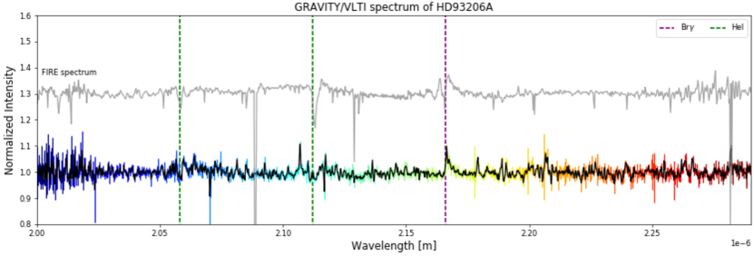
Figure 7: The figure displays the HD 93 206 A normalized spectrum obtained with GRAVITY. Different spectral bins are shown with different colors. Some of the main spectral features are identified and plotted with different colored dashed lines (see label on the plot). The FIRE spectrum is overplotted in gray and has been shifted from unity for better comparison with the GRAVITY one.

From the geometrical model, a separation between components in the outer binary of $\rho$=30.16$\pm$0.02 mas and a position angle of $\theta$=328.09$\pm$0.03^∘ were derived. These estimates agree with the values reported by Sana et al. (2014) using PIONIER ($\rho$=25.76$\pm$0.54 mas; $\theta$=331.31$\pm$1.45^∘) and SAM ($\rho$=28.05$\pm$5.41 mas; $\theta$=331.02$\pm$9.61^∘) observations taken in 2012, but with a precision between one and three orders of magnitude better, respectively. The SAM data derived a $\Delta K_{s}$=1.18$\pm$0.20 mag, however, our GRAVITY observations suggest a $\Delta K$=0.33$\pm$0.02 mag; a value that is closer to the $\Delta H$=0.42$\pm 0.18$ mag derived with the PIONIER observations. The angular separation between components of the binary is at the limit of the SAM angular-resolution ($\theta_{K}\sim$35 mas; for 8-meter telescopes). Thus, this could explain the poor performance of such technique to reliably recover the $\Delta K$ and separation of the system Aa-Ac. In addition, it highlights the importance of long-baseline interferometric observations, like our GRAVITY data to cover the relevant angular scales of systems like HD 93 206 A.

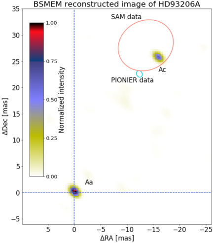
Figure 9: Reconstructed BSMEM image of HD 93 206 A. The components of the outer binary Aa-Ac are labeled on the figure. The color scale is also shown. Cyan and a red ellipses show the positions (within $\pm$1$\sigma$) of the Ac component according to the PIONIER and NACO/SAM values reported by Sana et al. (2014), respectively. Notice the large uncertainty ellipse of the SAM data compared to the precision of the long baseline interferometric data. The positional difference between the PIONIER and GRAVITY epochs is due to orbital motion.

With the position angles derived in 2012 and in this work, a projected North-West motion in the plane of the sky of component Ac relative to Aa is detected. Figure 9 displays a BSMEM (Buscher, 1994; Baron & Young, 2008) reconstructed image from our GRAVITY data together with the 2012 PIONIER and SAM positions marked on it. With only two astrometric points, it is not possible to derive a reliable orbital solution of the outer binary Aa-Ac (see Fig. 9). Nevertheless, (i) assuming a total mass of 90 M_⊙ (Leung et al., 1979; Morrison & Conti, 1980), (ii) a projected circular orbit with a mean separation at the aphelion of $\sim$30 mas, (iii) and a parallax to the Carina Nebula $\epsilon$ = 0.43 $\pm$ 0.02 (Smith, 2002), a rough orbital period of P = 61 $\pm$ 4 a is inferred. However, this estimate highly depends on the orbital elements of the system (e.g., eccentricity, inclination, mass, etc). For example, taken the previous constraints into account, a system projected in the plane of the sky with eccentric orbits e=0.5 and e=0.9, will result on P= 33 $\pm$ 2 a and P = 23 $\pm$ 1.6 a, respectively. These, still, poor constrains on the orbit support the necessity to carry out a proper GRAVITY monitoring program over, at least, the following 5 years, which together with the previous 2012 and 2016 data, would allow us to obtain more accurate estimates of the orbital motion of the system. The current Gaia TGAS (Gaia Collaboration et al., 2016a, b) lists for HD 93 206 a highly uncertain parallax of $\epsilon$ = 1.76 $\pm$ 0.62 mas, which includes, e.g., the distance to the Carina nebula within its 2$\sigma$ uncertainty. Once more a precise Gaia parallax measurement become available, it (combined with our new astrometric data) will further improve the constraints on the mass of the stellar components.

The general spectral signature of HD 93 206 A obtained with GRAVITY is consistent with the one taken with FIRE. In both spectra the Br$\gamma$ (2.1661 $\mu$m) shock tracer and HeI (2.058 $\mu$m and 2.112 $\mu$m) photospheric lines can be identified. The observed line profiles resemble the ones of late O- and early B-stars (see e.g., Hanson et al., 1996; Ghez et al., 2003; Tanner et al., 2006). This result confirms the presence of O9.7 I and O8 III stars in HD 93 206 A. However, some differences between the FIRE and GRAVITY spectra are observed. The HeI line at 2.112 $\mu$m in the FIRE spectrum appears to be an absorption feature with a well-defined peak and a wing shifted towards the red part of the spectrum. In contrast, the GRAVITY spectrum shows an absorption "W-shaped” profile. One of the most plausible causes of these line changes is the difference of the orbital phase in the compact binaries between both spectra (see e.g., Figure 1 and Figure 2 in Taylor et al., 2011). Variability of the spectral features in the visible part of the spectrum of HD 93 206 A was also reported by Morrison & Conti (1979) and Mayer et al. (2001), associating it to the double tight-binary nature of the source.

To test this scenario, Figure 8 shows normalized spectra in the H$\alpha$ line (0.656 $\mu$m) of HD 93 206 A obtained with FEROS (see Sec. 2.2). Considering the ephemeris published by Mayer et al. (2001) for Aa+Ac, we determine the orbital phases corresponding to each one of the spectroscopic binaries. The different phases are labeled to the left and right of each spectrum, respectively. At first glance, the variations of the profile on a day to day basis are very noticeable. The 2009 series of spectra (the four spectra from bottom to the top in Fig. 8) were obtained after the periastron passage of component Aa, but at more random orbital phases for component Ac. However, for the 2012 spectrum (the top data set in Fig. 8) shows Aa in an orbital phase just before the periastron and Ac close to the apastron. From a direct inspection of the overall shape and changes of the profile, we notice that while the Aa component is in an orbital phase close to the periastron, the line-peak profile remains similar in shape and amplitude. However, once the Aa component is at $\phi_{Aa}$ = 0.88, the line-peak profile becomes wider. From those observational changes, we infer that most of the narrow emission, close to the line peak, comes from the Aa component.

On the other hand, changes in the blue-shifted wing of H$\alpha$ appear to be related to component Ac. Notice how an absorption is observed in the wing at orbital phases close to the apastron ($\phi_{Ac}$ = 0.57 and $\phi_{Ac}$ = 0.43) and how it changes to a secondary emission peak before the periastron ($\phi_{Ac}$ = 0.89). However, besides the described changes in the line, without a detailed study of both binary components, it is still challenging to fully constrain which component of the binaries is contributing to the emission and/or absorption part of the profile. Future monitoring of the spectrum not only with GRAVITY but with other facilities like FEROS or UVES/VLT are necessary to complete the spectral analysis of the source.

Additionally to the observed changes in the FEROS data, it is important to highlight that the Br$\gamma$ line profile seen with GRAVITY is quite similar to the one of the H$\alpha$ line observed by Mayer et al. (2001) with the 1.4 m CAT telescope at La Silla Observatory and the bottom spectrum presented in Figure 8. Both the Br$\gamma$ and the H$\alpha$ lines have a peak emission of about 10-20% above the continuum with a sharp edge at the blue part of the spectrum and a extended wing towards the red. The Br$\gamma$ red wing extends up to $\sim$540 km/s, which is similar to the velocity of the H$\alpha$ red wing reported by Mayer et al. (2001). This line feature is a very strong indication for the presence of a stellar wind component.

Figure 8: H$\alpha$ spectra of HD 93 206 A obtained with FEROS. The figure displays 5 spectra at different orbital phases of the two spectroscopic binaries that compose HD 93 206 A. The morphology of the H$\alpha$ line clearly varies depending on the orbital phase. On the plot, each one of the epochs has been shifted vertically for a better representation.

The X-ray luminosity measured by Parkin et al. (2011) supports the presence of shock-tracers like Br$\gamma$ in the wind-wind collision regions of the quadruple system. However, the semi-detached nature of the binary Ac suggests the existence of a substantial case-B mass transfer (Leung et al., 1979) in which the transferred shock-heated plasma might be the main contributor to the observed Br$\gamma$ emission. A possibility to recognize which of the two binaries is the source of the spectral features is to disentangle the individual spectra of the binaries Aa and Ac. With the interferometric observations this is possible following the procedure detailed in Chesneau et al. (2014). This method relies, first, on the determination of the binary separation through a model fitting to all the data (like the one we applied in Sec. 3.1). Second, once the separation is determined, one can analyze the relative fluxes C_i of each one of the components per independent channel. Once C_i have been obtained, one can get the spectrum S_i of each component using the following expression:

$$S_{i}=\frac{C_{i}S_{*}}{\sum_{j=1}^{n}C_{j}}\,$$ (5)

where S_∗ is the spectrum of the source. After trying this method, we concluded that the data quality is not good enough to perform such analysis with the current data sets. Two main reasons are identified for this limitation: (i) the relatively large variation of the observables in adjacent channels across the bandpass and (ii) the relative faintness of the detected lines. However, future observations with GRAVITY at the UTs would allow us to perform this analysis.

To investigate the region in which the observed Br$\gamma$ line is formed, we computed the differential phases (Millour et al., 2006). Since we observe the target as a binary, the pseudo-continuum has a contribution from both components of the binary; thus, detecting a differential signature implies a relative change in the brightness of the components at the position of the line. Nevertheless, we do not detect any systematic change in this observable at the position of Br$\gamma$ compared to the pseudo-stellar continuum. As an example, Figure 10 displays the Br$\gamma$ differential phases of one of our GRAVITY data sets (similar trends are observed in the other ones). Since the flux ratio of the binaries appears to be preserved across the Br$\gamma$ profile, this line is produced at each of the internal binaries instead of being formed in a more extended region as a consequence of the interaction between both sub-systems Aa and Ac. However, this result is constrained by the SNR in our data. Considering an average 3$\sigma$ deviation of the differential phases of $\Delta_{\phi}^{3\sigma}\sim$15^∘, we derived an upper limit for the line-emitting regions of $p$=0.157 mas for a baseline of $B$=120 m, following the next expression (Kraus, 2012):

$$p=\frac{\Delta_{\phi}^{3\sigma}}{2\pi}.\frac{\lambda}{B}\,.$$ (6)

Since the observed lines are highly variable depending on the different orbital phases of the spectroscopic binaries, future observations of this source with higher SNR are required to systematically determine the astrometric offsets associated with the different orbital phases of the inner binaries. With at least 3.5 mag more in sensitivity, GRAVITY using the 8-meter Unit Telescopes will provide us the required capabilities to (i) monitor the temporal changes in the lines, (ii) to disentangle the spectra of the spectroscopic binaries and (iii) to provide an estimation of the orbital solution for the internal binaries (with a expected differential phase calibration of $\Delta_{\phi}^{3\sigma}\sim$2^∘ or 20 $\mu$as at 120 m baselines).

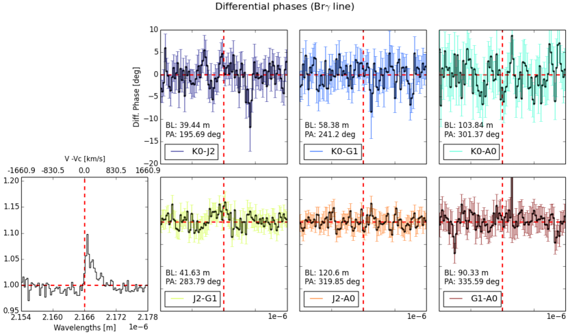
Figure 10: The figure displays the differential phases per baseline at the position of the Br$\gamma$ line for one of our GRAVITY data sets (MJD: 57557.046). The left most panel shows the normalized total spectrum of the source. The upper axis displays the relative velocity from the nominal position of the line. The continuum baseline is plotted with a red dashed line. The differential phases are plotted in different colors depending on the baseline (see labels on the figure). The baseline length and its position angle are labeled at each panel. The nominal position of the Br$\gamma$ line is shown with a vertical red dashed line. The zero-point in the differential phases is displayed at each panel with an horizontal dashed line. All the panels share the same scale in the horizontal axis.

5 Conclusions

This work demonstrates the enormous scientific capabilities of the new GRAVITY instrument fo the characterization of multiplicity in massive systems. The system HD 93 206 A is a showcase for this kind of analysis. It represents the first object of a future survey with GRAVITY. In particular, we have obtained the following results for HD 93 206 A:

• We characterize the relative astrometry between the spectroscopic binaries Aa and Ac with a precision of tens of microarcseconds. This corresponds to a dramatic improvement of one and three orders of magnitude compared to the previous astrometric measurements with PIONIER/VLTI and NACO/SAM, respectively. The derived separation between Aa and Ac is $\rho\sim$30 mas with a position angle PA$\sim$328^∘ and a $\Delta K$=0.32 mag, with a detected projected motion towards the North-West from the 2012 data. This demonstrates the gravitational boundedness between the two SBs and provides a rough estimate of their mutual orbital period of P $\leq$ 60 years. The precise determination of the Aa-Ac astrometry over several future epochs ($\sim$5 years) will be crucial to constrain the fundamental parameters of the system, its formation history and to predict whether the system is long-term (over a few million years) stable or not.

• From the CANDID analysis of our GRAVITY observations, we derived a maximum magnitude difference of $\Delta K\sim$5 mag to detect companions, with a 3$\sigma$ confidence level, in a range of 3 to 50 mas around the primary. This represents an increment in sensitivity of $\sim$2 mag from the one achieved with PIONIER/VLTI. The current surveys with the 1st generation of VLTI instruments have a limiting $\Delta_{m}\sim$ 3 - 4 mag between binary components with separations from 1 to 10 mas. Thus, the present result confirms GRAVITY as a unique instrument to explore a new parameter space in the characterization of massive multiple systems. Here, we have demonstrated the superb calibration and sensitivity of the single-field mode of the instrument. Nevertheless, the expected improvement in the GRAVITY performance (particularly its complete integration with the 8 m Unit Telescopes) over the next year, in combination with the so-called “dual-field” mode of the instrument, will provide us the opportunity to look for companions in stars as faint as $\sim$10 mag with the ATs and $\sim$16 mag with the UTs, letting us to completely characterize systems like HD 93 206.

• A dedicated Principal Component Analysis of the GRAVITY data allowed us to extract the calibrated spectrum of the source in which shock tracers (Br$\gamma$) and stellar (HeI) lines are observed. The detected spectral features have a maximum intensity $\sim$10% above the pseudo-stellar continuum. Complementary FIRE data supports variability of the $K-$band lines and visible FEROS spectra indicate that the daily variability is linked to the motion of the multiple components of the quadruple. It appears that changes around the peak of the H$\alpha$ are associated to the Aa component, while changes in the wings correspond to the Ac component.

• We constrain the near-infrared wind-wind collision region associated to the observed X-ray emission of the source. From our differential phase analysis at the position of Br$\gamma$, we confirm that it is formed in very compact regions inside the inner binaries and not from a more extended region between both sub-systems Aa and Ac. This is consistent with previous models which suggest that the X-ray emission is arising mostly within the spectroscopic binaries, in particular from component Ac. With the current data we could not confirm which of the two spectroscopic binaries is the main X-ray emitter. However, from the 3$\sigma$ standard deviation of the differential phases from the continuum baseline, we infer an upper limit for the line-emitting regions of p$\sim$0.157 mas (0.37 AU).

  Future observations with the UTs in “single-field” mode will provide us a calibration of $\Delta\phi\sim$1^∘ to constrain the line-emitting region up to scales of 20 $\mu$as (0.05 AU at the distance of the source). If the detected changes in H$\alpha$ are applicable to Br$\gamma$, detecting systematic changes in the differential phases would allow us to disentangle the astrometric motion of the individual components within the spectroscopic binaries. Monitoring projected astrometric motions combined with spectroscopic data and a proper model of the emission line variability will let us to characterize, for the first time, the fundamental parameters of the individual components in the system. This information would provide the mass distribution among the components, test coplanarity among the different orbital planes and confront the different formation scenarios in this kind of systems.

Appendix A SNR distributions of the interferometric observables

References

- Absil et al. (2011) Absil, O., Le Bouquin, J.-B., Berger, J.-P., et al. 2011, A&A, 535, A68
- Allen (2015) Allen, C. 2015, Revista Mexicana de Astronomia y Astrofisica Conference Series, 46, 40
- Apai et al. (2007) Apai, D., Bik, A., Kaper, L., Henning, T., & Zinnecker, H. 2007, ApJ, 655, 484
- Bally & Zinnecker (2005) Bally, J., & Zinnecker, H. 2005, AJ, 129, 2281
- Barbá et al. (2010) Barbá, R. H., Gamen, R., Arias, J. I., et al. 2010, Revista Mexicana de Astronomia y Astrofisica Conference Series, 38, 30
- Baron & Young (2008) Baron, F., & Young, J. S. 2008, Society of Photo-Optical Instrumentation Engineers (SPIE) Conference Series, 7013, 3
- Blind et al. (2014) Blind, N., Eisenhauer, F., Haug, M., et al. 2014, in Proc. SPIE, Vol. 9146, Optical and Infrared Interferometry IV
- Bochanski et al. (2009) Bochanski, J. J., Hennawi, J. F., Simcoe, R. A., et al. 2009, PASP, 121, 1409
- Bonneau et al. (2011) Bonneau, D., Delfosse, X., Mourard, D., et al. 2011, A&A, 535, A53
- Bonneau et al. (2006) Bonneau, D., Clausse, J.-M., Delfosse, X., et al. 2006, A&A, 456, 789
- Bonnell & Bastien (1992) Bonnell, I., & Bastien, P. 1992, ApJ, 401, L31
- Bonnell & Bate (2005) Bonnell, I. A., & Bate, M. R. 2005, MNRAS, 362, 915
- Bonnell & Bate (2006) —. 2006, MNRAS, 370, 488
- Broos et al. (2011) Broos, P. S., Townsley, L. K., Feigelson, E. D., et al. 2011, ApJS, 194, 2
- Buscher (1994) Buscher, D. F. 1994, in IAU Symposium, Vol. 158, Very High Angular Resolution Imaging, ed. J. G. Robertson & W. J. Tango, 91
- Chesneau et al. (2014) Chesneau, O., Meilland, A., Chapellier, E., et al. 2014, A&A, 563, A71
- Chini et al. (2012) Chini, R., Hoffmeister, V. H., Nasseri, A., Stahl, O., & Zinnecker, H. 2012, MNRAS, 424, 1925
- Close et al. (2013) Close, L. M., Males, J. R., Morzinski, K., et al. 2013, ApJ, 774, 94
- Colavita et al. (1999) Colavita, M. M., Wallace, J. K., Hines, B. E., et al. 1999, ApJ, 510, 505
- Cushing et al. (2004) Cushing, M. C., Vacca, W. D., & Rayner, J. T. 2004, PASP, 116, 362
- Dawson & Aguilar (1937) Dawson, B. H., & Aguilar, F. 1937, Observatory Astronomical La Plata Series Astronomies, 6, 86
- Eisenhauer et al. (2008) Eisenhauer, F., Perrin, G., Brandner, W., et al. 2008, SPIE Conference Series - Optical and Infrared Interferometry, 7013, 70132A
- Eisenhauer et al. (2011) —. 2011, The Messenger, 143, 16
- Foreman-Mackey et al. (2013) Foreman-Mackey, D., Hogg, D. W., Lang, D., & Goodman, J. 2013, PASP, 125, 306
- Fujii & Portegies Zwart (2011) Fujii, M. S., & Portegies Zwart, S. 2011, Science, 334, 1380
- Gaia Collaboration et al. (2016a) Gaia Collaboration, Brown, A. G. A., Vallenari, A., et al. 2016a, A&A, 595, A2
- Gaia Collaboration et al. (2016b) Gaia Collaboration, Prusti, T., de Bruijne, J. H. J., et al. 2016b, A&A, 595, A1
- Gallenne et al. (2015) Gallenne, A., Mérand, A., Kervella, P., et al. 2015, A&A, 579, A68
- Ghez et al. (2003) Ghez, A. M., Duchêne, G., Matthews, K., et al. 2003, ApJ, 586, L127
- Gillessen et al. (2010) Gillessen, S., Eisenhauer, F., Perrin, G., et al. 2010, SPIE: Optical and Infrared Interferometry II, 7734, 77340Y
- GRAVITY Collaboration et al. (2017) GRAVITY Collaboration, Abuter, R., Accardo, M., et al. 2017, Submmitted to A&A: ArXiv e-prints: 1705.02345
- Hanson et al. (1996) Hanson, M. M., Conti, P. S., & Rieke, M. J. 1996, ApJS, 107, 281
- Hillwig et al. (2006) Hillwig, T. C., Gies, D. R., Bagnuolo, Jr., W. G., et al. 2006, ApJ, 639, 1069
- Ivezic et al. (2014) Ivezic, Z., Connolly, A. J., VanderPlas, J. T., & Gray, A. 2014, Statistics, Data Mining, and Machine Learning in Astronomy: A Practical Python Guide for the Analysis of Survey Data (Princeton, NJ, USA: Princeton University Press)
- Jolliffe (1986) Jolliffe, I. 1986, Principal Component Analysis (New York, NY, USA: Springer Verlag)
- Kraus (2012) Kraus, S. 2012, in Proc. SPIE, Vol. 84451H, Optical and Infrared Interferometry III, 84451H
- Kraus et al. (2009) Kraus, S., Weigelt, G., Balega, Y. Y., et al. 2009, A&A, 497, 195
- Krumholz et al. (2009) Krumholz, M. R., Klein, R. I., McKee, C. F., Offner, S. S. R., & Cunningham, A. J. 2009, Science, 323, 754
- Lachaume & Berger (2013) Lachaume, R., & Berger, J.-P. 2013, MNRAS, 435, 2501
- Lacour et al. (2008) Lacour, S., Jocou, L., Moulin, T., et al. 2008, SPIE: Optical and Infrared Interferometry, 7013, 701316
- Lapeyrere et al. (2014) Lapeyrere, V., Kervella, P., Lacour, S., et al. 2014, SPIE Conference Series - Optical and Infrared Interferometry IV, 9146, 91462D
- Leung et al. (1979) Leung, K.-C., Moffat, A. F. J., & Seggewiss, W. 1979, ApJ, 231, 742
- Maeder & Behrend (2002) Maeder, A., & Behrend, R. 2002, in Astronomical Society of the Pacific Conference Series, Vol. 267, Hot Star Workshop III: The Earliest Phases of Massive Star Birth, ed. P. Crowther, 179
- Mason et al. (1998) Mason, B. D., Gies, D. R., Hartkopf, W. I., et al. 1998, AJ, 115, 821
- Mason et al. (2001) Mason, B. D., Wycoff, G. L., Hartkopf, W. I., Douglass, G. G., & Worley, C. E. 2001, AJ, 122, 3466
- Mayer et al. (2001) Mayer, P., Lorenz, R., Drechsel, H., & Abseim, A. 2001, A&A, 366, 558
- Millour et al. (2006) Millour, F., Vannier, M., Petrov, R. G., et al. 2006, in EAS Publications Series, Vol. 22, EAS Publications Series, ed. M. Carbillet, A. Ferrari, & C. Aime, 379–388
- Monin et al. (2007) Monin, J.-L., Clarke, C. J., Prato, L., & McCabe, C. 2007, "Protostars and Planets V: Disk Evolution in Young Binaries: From Observations to Theory", Reipurth, b. and Jewitt, d. and Keil, k. edn. (Tucson, AZ, USA: University of Arizona Press), 395–409
- Morrison & Conti (1979) Morrison, N. D., & Conti, P. S. 1979, Mass Loss and Evolution of O-Type Stars; eds. Conti, P. S. and De Loore, C. W. H., 83, 277
- Morrison & Conti (1980) —. 1980, ApJ, 239, 212
- Nelan et al. (2004) Nelan, E. P., Walborn, N. R., Wallace, D. J., et al. 2004, AJ, 128, 323
- Parkin et al. (2011) Parkin, E. R., Broos, P. S., Townsley, L. K., et al. 2011, ApJS, 194, 8
- Peter et al. (2012) Peter, D., Feldt, M., Henning, T., & Hormuth, F. 2012, A&A, 538, A74
- Sana et al. (2014) Sana, H., Le Bouquin, J.-B., Lacour, S., et al. 2014, ApJS, 215, 15
- Schertl et al. (2003) Schertl, D., Balega, Y. Y., Preibisch, T., & Weigelt, G. 2003, A&A, 402, 267
- Simcoe et al. (2013) Simcoe, R. A., Burgasser, A. J., Schechter, P. L., et al. 2013, PASP, 125, 270
- Smith (2002) Smith, N. 2002, MNRAS, 337, 1252
- Smith (2006) —. 2006, MNRAS, 367, 763
- Sota et al. (2014) Sota, A., Maíz Apellániz, J., Morrell, N. I., et al. 2014, ApJS, 211, 10
- Sota et al. (2011) Sota, A., Maíz Apellániz, J., Walborn, N. R., et al. 2011, ApJS, 193, 24
- Stickland & Lloyd (2000) Stickland, D. J., & Lloyd, C. 2000, The Observatory, 121, 1
- Tallon-Bosc et al. (2008) Tallon-Bosc, I., Tallon, M., Thiébaut, E., et al. 2008, in Proc. SPIE, Vol. 7013, Optical and Infrared Interferometry, 70131J
- Tanner et al. (2006) Tanner, A., Figer, D. F., Najarro, F., et al. 2006, ApJ, 641, 891
- Tatulli et al. (2007) Tatulli, E., Millour, F., Chelli, A., et al. 2007, A&A, 464, 29
- Taylor et al. (2011) Taylor, W. D., Evans, C. J., Sana, H., et al. 2011, A&A, 530, L10
- Townsley et al. (2011) Townsley, L. K., Broos, P. S., Chu, Y.-H., et al. 2011, ApJS, 194, 15
- Vacca et al. (2003) Vacca, W. D., Cushing, M. C., & Rayner, J. T. 2003, PASP, 115, 389
- Walborn (1995) Walborn, N. R. 1995, Revista Mexicana de Astronomia y Astrofisica Conference Series, 2, 51
- Weigelt et al. (1999) Weigelt, G., Balega, Y., Preibisch, T., et al. 1999, A&A, 347, L15
- Zinnecker & Bate (2002) Zinnecker, H., & Bate, M. R. 2002, in Astronomical Society of the Pacific Conference Series, Vol. 267, Hot Star Workshop III: The Earliest Phases of Massive Star Birth, ed. P. Crowther, 209
- Zinnecker & Yorke (2007) Zinnecker, H., & Yorke, H. W. 2007, ARA&A, 45, 481