HIFI Spectroscopy of submm Lines in Nuclei of Actively Star Forming Galaxies
Abstract
We present a systematic survey of multiple velocity-resolved H2O spectra using Herschel/HIFI towards nine nearby actively star forming galaxies. The ground-state and low-excitation lines (E130 K) show profiles with emission and absorption blended together, while absorption-free medium-excitation lines (130 K E350 K) typically display line shapes similar to CO. We analyze the HIFI observation together with archival SPIRE/PACS H2O data using a state-of-the-art 3D radiative transfer code which includes the interaction between continuum and line emission. The water excitation models are combined with information on the dust- and CO spectral line energy distribution to determine the physical structure of the interstellar medium (ISM). We identify two ISM components that are common to all galaxies: A warm ( K), dense () phase which dominates the emission of medium-excitation H2O lines. This gas phase also dominates the FIR emission and the CO intensities for . In addition a cold ( K), dense () more extended phase is present. It outputs the emission in the low-excitation H2O lines and typically also produces the prominent line absorption features. For the two ULIRGs in our sample (Arp 220 and Mrk 231) an even hotter and more compact (R pc) region is present which is possibly linked to AGN activity. We find that collisions dominate the water excitation in the cold gas and for lines with K and K in the warm and hot component, respectively. Higher energy levels are mainly excited by IR pumping.
Subject headings:
galaxies: low-redshift, high-redshift — galaxies: formation — galaxies: evolution — galaxies: starbursts — radio1. Introduction
Galactic nuclei play a key role in our understanding of galactic evolution. An important method to determine their physical and chemical conditions is the analysis of molecular emission lines from the interstellar medium (ISM). Of particular interest is the water molecule, which has been demonstrated to have uniquely powerful potential of deriving information on the ISM of external galaxies (e.g., González-Alfonso et al., 2010). The abundance of water in the gas phase (, )) in quiescent molecular clouds is quite low as suggested by studies in the Milky Way (e.g., , Caselli et al., 2010). But water becomes one of the most (third) abundant species in the shock-heated regions (e.g., Bergin et al., 2003; González-Alfonso et al., 2013) and in the dense warm regions in which radiation from newly-formed stars raises the dust temperature above the ice evaporation temperature (e.g., Cernicharo et al., 2006b). Therefore, unlike other molecular gas tracers traditionally used to study the dense, star-forming (SF) ISM in extragalactic systems (such as CO and HCN), water probes the gas exclusively associated with SF regions or heated in the extreme environment of active galactic nuclei (AGN). Because of its complex energy level structure and large level spacing, possesses a large number of rotation lines that lie mostly in the submillimeter (submm) and far-infrared (FIR) wavelength regime. These lines can be very prominent in actively star-forming galaxies with intensities comparable to those of CO lines - much more prominent than other dense gas tracers such as HCN (e.g., van der Werf et al., 2011). The water lines do not only probe the physical conditions of the gas phase ISM (such as gas density and kinetic temperature), but also provide important clues on the dust IR radiation density as both collision with hydrogen molecule and IR pumping are important for their excitation (e.g., Weiß et al., 2010; González-Alfonso et al., 2012, 2014). The high-excitation water lines can even be used to reveal the presence of extended infrared-opaque regions in galactic nuclei and probe their physical conditions (van der Werf et al., 2011). This offers a potential diagnostic to distinguish AGN from starburst activity. Observations of water also shed light on the dominant chemistry in nuclear regions (e.g., Bergin et al., 1998, 2000; Melnick et al., 2000) as water could be a major reservoir of gas-phase interstellar oxygen (e.g., Cernicharo et al., 2006a). Overall, water provides a unique tool to probe the physical and chemical processes occurring in the galaxy nuclei and their surroundings (e.g., van der Werf et al., 2011; González-Alfonso et al., 2014).
However, previous observations of water in nearby extragalactic systems suffered great limitations. Ground-based observations of water in nearby galaxies have been limited to radio maser transitions (such as the famous 22 GHz water line) or to a few systems with significant redshift (e.g., Combes & Wiklind, 1997; Cernicharo et al., 2006b; Menten et al., 2008) due to the absorption by terrestrial atmospheric water vapour. Earlier satellite missions, such as ODIN and SWAS, did not have enough collecting area to detect the relatively faint ground transitions of water in external galaxies. ISO and, more recently, Spitzer have provided the first systematic studies of water in the far-infrared regime (e.g., Fischer et al., 1999; González-Alfonso et al., 2004). These missions, however, did not cover the frequencies of the molecule’s ground-state transitions and other low-excitation111Throughout this paper, we use the term low-excitation for H2O lines with upper level energies K, medium-excitation for lines with K and high-excitation for lines with K. lines. These low-excitation water transitions provide crucial information on the widespread diffuse medium in galaxies (Weiß et al., 2010; van der Tak et al., 2016). Only with the launch of Herschel222Herschel is an ESA space observatory with science instruments provided by European-led Principal Investigator consortia and with important participation from NASA., with its large collecting area, have these transitions become accessible in the nearby universe (e.g., González-Alfonso et al., 2010; Weiß et al., 2010). Yet, SPIRE (and also PACS) on-board Herschel does not provide the spectral resolution to obtain velocity resolved spectra and only the integrated line intensities (or barely resolved spectra) can be obtained from these observations.
High velocity resolution spectroscopy with Herschel’s Heterodyne Instrument for the Far Infrared (HIFI), however, allows us to derive detailed information on the shapes of H2O lines, which is critical because emission and absorption are often mixed in water line profiles (Weiß et al., 2010). This implies that the modest spectral resolution of the Herschel/SPIRE spectroscopy results in severe limitations for the detections of low-excitation lines and limits the construction of excitation models, since emission and absorption from different ISM components along the line of sight are averaged. Recently, water has been detected in high- sources with both high spectral and spatial resolution afforded by ALMA and NOEMA (e.g., Omont et al., 2011, 2013; Combes et al., 2012; Yang et al., 2016). The results confirm that lines are among the strongest molecular lines in high- ultra-luminous starburst galaxies, with intensities almost comparable to those of the high- CO lines (e.g., Omont et al., 2013; Yang et al., 2016). In order to obtain a better understanding of observed water spectra in the early universe, a comprehensive analysis of water line shapes in the local universe is required. Only with HIFI, we are able to investigate multiple water transitions resulting from levels with a wide range of energies in nearby galaxies in more detail than ever before.
The observed water line profiles provide crucial information on the geometry, dynamics and physical structure of the ISM. However, retrieving these information is not straightforward, because most water lines have high optical depth (e.g., Emprechtinger et al., 2012; Poelman et al., 2007; Poelman & van der Tak, 2007) so that column densities cannot be accurately derived from the observed line intensities alone. The excitation of water is also more complicated than other traditional gas tracers (e.g., CO, CS) as IR pumping has to be taken into account. The gas-phase could be a major coolant of the dense, star-forming ISM in case it is mainly collisionally excited. Yet, the relative importance of collision and IR pumping on the excitation of water in extragalactic sources has not achieved a full understanding. Interstellar chemistry will benefit from an accurate knowledge of water abundances, the derivation of which requires detailed modelling of H2O’s excitation of the rotational levels. Hence, to extract the underlying physical properties of the ISM (both gas and dust), to investigate the relative contribution of the two excitation channels and derive chemical abundances, a detailed modelling of the water excitation is required.
In this paper we present velocity-resolved HIFI spectroscopy of multiple FIR lines (with upper energy K) in a sample of nine local galaxies with different nuclear environments. We analyse the data using a 3D, non-LTE radiative transfer code. Our main goal is to deepen our understand of the water excitation and to explore as a diagnostic tool to probe the physical and chemical conditions in the nuclei of active star-forming galaxies. We present our sample, observations and data reduction in Section 2. A discussion of the line shapes is presented in Section 3. A description of our modelling method and a summary of our general model results is given in Section 4. In Section 5 we discuss the contributions from collisions and IR pumping on the excitation of water as well as the resulting shape of the SLEDs, and establish a luminosity relation. Our conclusions are summarised in Section 6.
2. Observation
Our sample is selected from the HEXGAL (Herschel ExtraGALactic) key project (PI: Güsten). HEXGAL is a project that aims to study the physical and chemical composition of the ISM in galactic nuclei, utilising the very high spectral resolution of the HIFI instrument. Our sample consists of a total of nine galaxies and has been selected to cover a diversity of nuclear environments ranging from pure nuclear starburst galaxies (such as M82, NGC 253) to starburst nuclei that also host an AGN (such as NGC 4945) to AGN dominated environments (such as Mrk 231) and to major mergers with even higher IR luminosity (such as Arp 220). The source names, systemic velocities, distances, FIR (m, Helou et al., 1985) luminosities and galaxy types are given in Table 1. The FIR luminosities are computed by integrating our fitted SEDs over the wavelength range m (see Section 4.1.2 for more details on the dust SED fitting).
| Galaxy | vLSR | distance | (FWHM=40″) | RA | Dec | type |
|---|---|---|---|---|---|---|
| [Mpc] | [] | h m s.s | ′ ′′ | |||
| M82 | 203 | 3.9 | 9.74 | 09 55 52.2 | +69 40 46 | SB |
| NGC 253 | 243 | 3.2 | 9.47 | 00 47 33.1 | 25 17 17 | SB |
| NGC 4945 | 563 | 3.9 | 10.70 | 13 05 27.4 | 49 28 05 | SB/AGN |
| NGC 1068 | 1137 | 12.6 | 10.32 | 02 42 40.7 | 00 00 47 | AGN/SB |
| Cen A | 547 | 3.7 | 9.23 | 13 25 27.6 | 43 01 08 | AGN/SB |
| Mrk 231 | 12642 | 186 | 12.19 | 12 56 14.2 | +56 52 25 | AGN/SB |
| Antennae | 1705 | 21.3 | 9.69 | 12 01 54.8 | 18 52 55 | SB, Major Merger |
| NGC 6240 | 7339 | 106 | 11.81 | 16 52 58.8 | +02 24 03 | AGN/SB, Major Merger |
| Arp 220 | 5434 | 78.7 | 11.98 | 15 34 57.2 | +23 30 11 | SB/AGN, Major Merger |
Note. — The FIR luminosities are computed by integrating our fitted SEDs over the wavelength range m. The last column indicates whether the IR luminosity of a galaxy is dominated by starburst (SB), AGN or both, and whether the galaxy is a major merger.
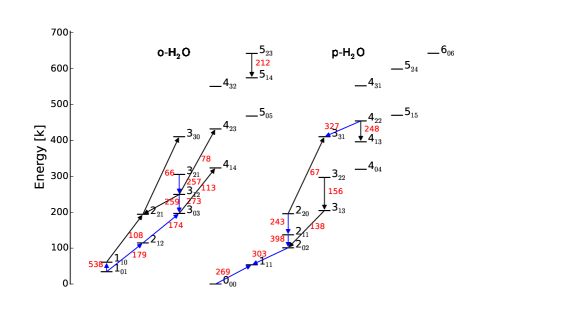
We have utilised HIFI to observe five to ten carefully selected (both ortho- and para-) water transitions. Fig. 1 shows the water energy diagram. Transitions observed with HIFI are indicated by blue arrows whereas black arrows denote additional lines covered by Herschel SPIRE and PACS that are also included in our modelling (more details in Section 4.1.1). Our observed lines cover a wide energy range, from low-excitation transitions (with K) to medium-excitation transitions (with K) to high-excitation transitions ( K). Table. 2 reports our selected water transitions, the line frequencies, the energies of upper levels, the corresponding HIFI beam sizes, the galaxies toward which each line has been observed, whether emission or absorption is found and the detection rate. The frequencies of our selected lines almost span the full HIFI frequency coverage of Bands 1-5 ( GHz) and Band 6 ( GHz). The angular resolutions changes from for the o- 557 GHz line to for the o- 1717 GHz line. We observed each galaxy towards a single position given in Table 1. Thus, except for the most distant sources (Arp 220, Mrk 231 and NGC 6240), only the nuclear region is covered by our pointed observations.
| Line | Freq. | observed galaxies | Emission or Absorptiona | detection rateb | ||
|---|---|---|---|---|---|---|
| [GHz] | [K] | [′′] | ||||
| p- (111-000) | 1113 | 53.4 | 19 | all | absorption, emission | 7/9 |
| o- (110-101) | 557 | 61.0 | 40 | all | absorption, emission | 8/9 |
| p-H2O (202-111) | 988 | 100.8 | 22 | all | emission | 8/9 |
| o-H2O (212-101) | 1670 | 114.4 | 13 | NGC 253, NGC 4945 | absorption | 2/2 |
| p-H2O (211-202) | 752 | 136.9 | 28 | all | emission | 6/9 |
| p-H2O (220-211) | 1229 | 195.9 | 17 | NGC253, CenA | emission | 1/2 |
| o-H2O (303-212) | 1717 | 196.8 | 12 | NGC 253, NGC 4945 | absorption, emission | 2/2 |
| o-H2O (312-303) | 1097 | 249.4 | 19 | all but NGC 1068 | emission | 6/8 |
| o-H2O (321-312) | 1163 | 305.3 | 18 | NGC 4945/253/6240, CenA | emission | 2/4 |
| p-H2O (422-331) | 916 | 454.3 | 23 | all | emission | 1/9 |
Note. — whether a line has been detected in emission, absorption, or both in our sample galaxies; the number of detected galaxies divided by the number of observed galaxies.
The data was obtained between March 2010 and September 2012, in a total of 124 hours of integration time. The dual beamswitch mode was used with a wobbler throw of 3 for all observations. The data was recorded using the wide-band acousto-optic spectrometer, consisting of four units with a bandwidth of 1 GHz each, covering the 4 GHz intermediate frequency band (IF) for each polarization with a spectral resolution of 1 MHz. Our spectra were calibrated using HIPE333Version 10.0.0. HIPE is a joint development by the Herschel Science Ground Segment Consortium, consisting of ESA, the NASA Herschel. and then exported to CLASS444http://www.iram.fr/IRAMFR/GILDAS format with the shortest possible pre-integration. For each scan we computed the underlying continuum using the line-free channels of a combined 4 GHz spectrum from the four sub-bands. Then a first-order baselines was subtracted from each individual sub-band (in the cases where the signal spans over more than one sub-band, the nearby sub-bands were merged before subtracting the baselines). Next the baseline-subtracted sub-bands in each scan were combined and the continuum level was added again. The noise-weighted spectra from two polarizations (H and V) were thereafter averaged. Note that the continuum radiation enters the receiver through both sidebands while the line is only in one sideband. Therefore the continuum used in our analysis (and for our figures) represents half of the value actually measured by HIFI. The o- () 1163 GHz line of NGC 4945 was found to partly blend with CO () line, we therefore have estimated the CO () line profile from the APEX CO () line and subtracted it from the spectra.
3. Spectral Results and Analysis
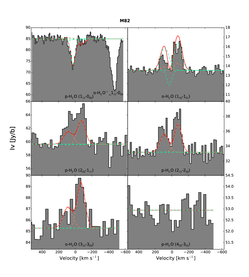
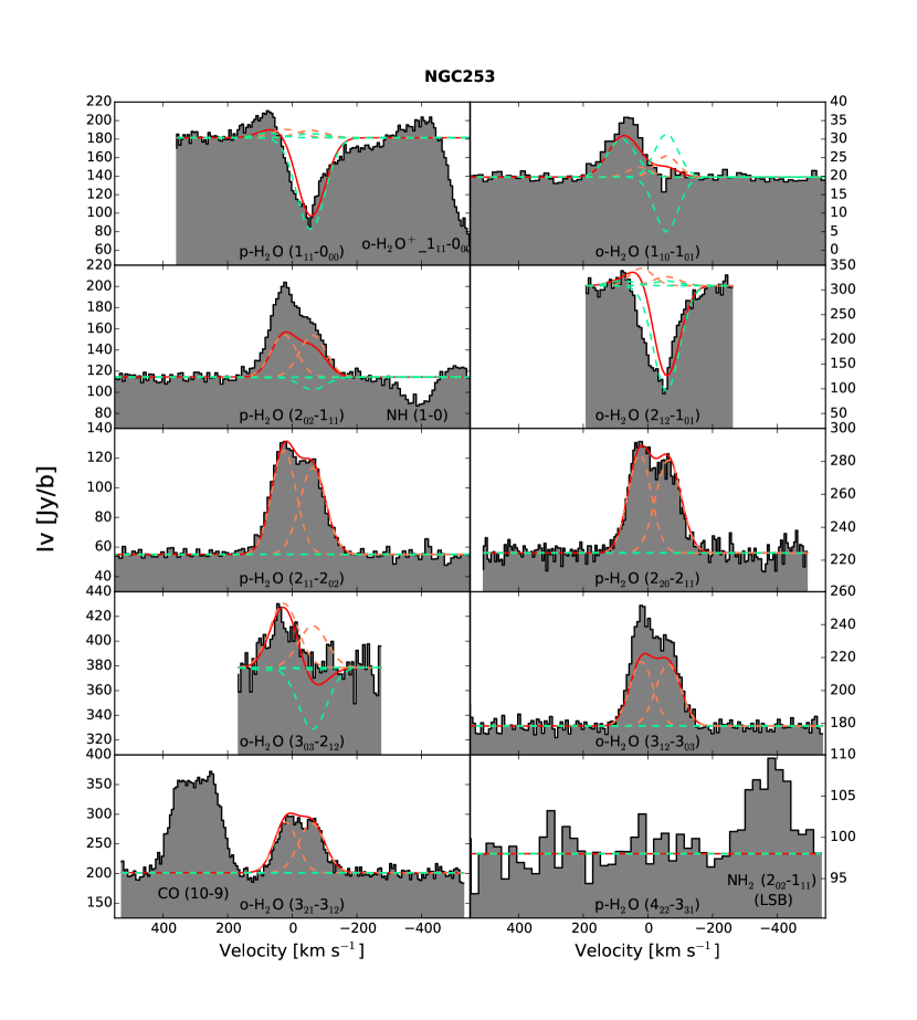
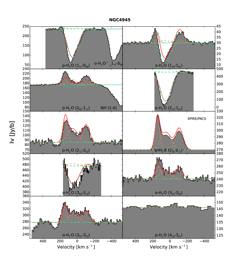
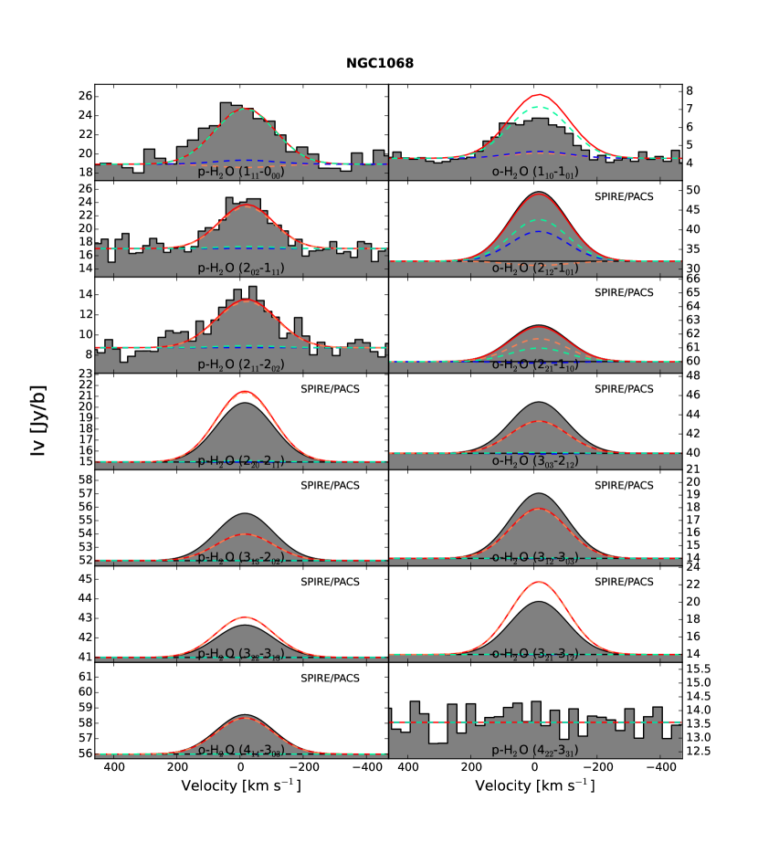
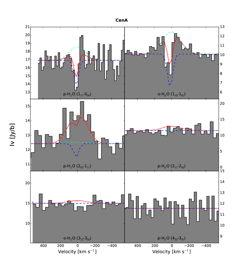
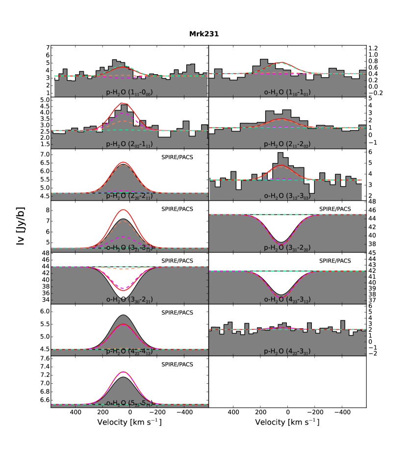
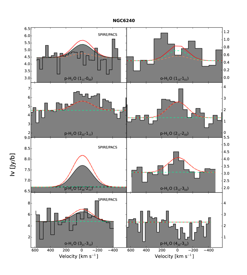
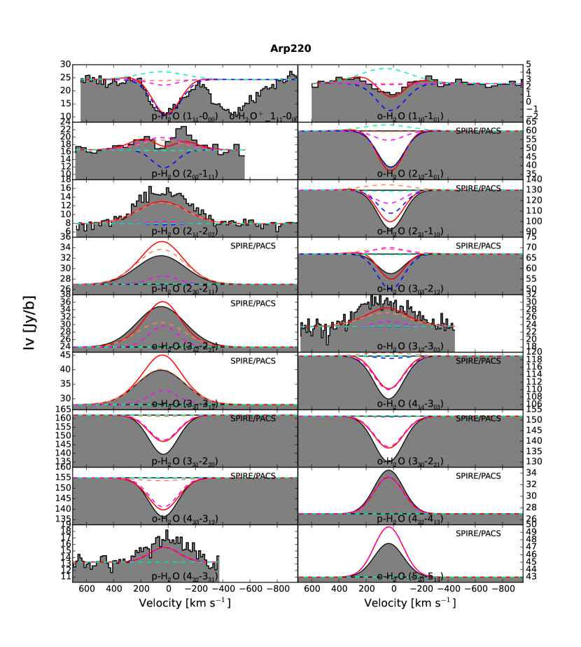
We detected strong water emission and absorption in all galaxies except for the Antennae, which has no detection in any line. Our HIFI spectra are presented in Figs. 11, 12, 13, 14, 15, 16, 17, 18. The velocity scale on each panel is relative to the systemic velocity listed in Table 1. Except for a few sources (Mrk 231, NGC 1068 and NGC 6240), a wide variety of line shapes is observed for most galaxies in our sample (e.g., NGC 4945, NGC 253, M82). In the latter cases emission and absorption features are often blended. Unlike line profiles from multiple transitions of other molecules (such as CO), the line profiles of water cannot be assumed to be similar.
3.1. Line Shapes
3.1.1 Emission Lines
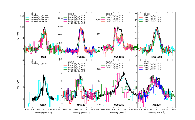
A few of the lines (indicated by blue downward solid arrows in Fig. 1) are always detected in emission. They include a low-excitation line (p- ()), four medium-excitation lines (o- (), o- (), p- (), and p- ()) and a high-excitation line (p- ()). These emission lines display similar line shapes among each other and also show a good correspondence to the line profile of CO. Fig. 2 presents the CO () line obtained by APEX555This publication is based in part on data acquired with the Atacama Pathfinder Experiment (APEX). APEX is a collaboration between the Max-Planck-Institut für Radioastronomie, the European Southern Observatory, and the Onsala Space Observatory. () or JCMT () overlaid on the HIFI detected emission lines. All H2O line profiles in Fig. 2 have been scaled to the peak of the CO line for better visualisation of the line shapes. One can see that, except for NGC 253 whose water line profile is slightly narrower than the CO () profile (see Appendix B for more discussions on this), water is often detected over the full velocity range of CO. This suggests that water is as widespread as CO and likely traces the bulk of the molecular gas in the central region of galaxies.
The closest resemblance is found between the CO and four medium-excitation lines which have K above the ground-state. The high-excitation emission line - p- () (with K) - which has been detected only in Arp 220, displays a narrower velocity dispersion () compared with that of the CO and medium-excitation lines () (see Fig. 2). The low-excitation emission line p- () (with K) often exhibits diminished emission compared to CO at the velocities where ground-state absorptions are detected, implying that the line is partly absorbed at the same velocities.
3.1.2 Absorption Lines
We have found four lines with absorption features in at least one galaxy of our sample. These are the p- ground-state () line, the o- ground-state () line, the o- () line and the o- () line (see blue upward arrows in Fig. 1). Except for the o- () line that has K, all other absorption lines occur between low energy levels ( K). The two ground-state lines show absorptions towards all galaxies except for Mrk 231, NGC 1068 and NGC 6240. We further find that the absorption depth of the o- ground-state line is usually much weaker () than that of the p- ground-state line. The other two absorption lines (o- () and o- ()) have only been observed towards NGC 253 and NGC 4945. Their line shapes are similar to the absorption feature of the p- ground-state line.
The observed absorption features can appear to be either broad and deep (e.g., Arp220 and NGC 4945), or narrow and shallow (e.g., Cen A). In some galaxies (e.g., NGC 253 and NGC 4945), the low-excitation absorption feature covers a velocity range matching that of medium-excitation emission lines, while in some other galaxies (e.g., M82) the absorption feature occurs at a velocity that does not show emission in other lines.
Absorption and emission features are often found to be blended. Especially for the o- ground-state line, strong emission is detected in all of our sample galaxies, in particular towards the high and low velocity wings of the line profile. Conspicuous emission features also show up in the p- ground-state line in a few galaxies (e.g., NGC 253 and NGC 1068), although they appear to be much weaker. Finally, we find the observed global line profiles with absorption and emission blended together are best explained by an emission profile similar to the medium-excitation lines modified by absorption components from foreground gas. It is therefore tempting to speculate that the lack of absorption at certain velocities has a geometrical origin, i.e., gas at these velocities is located outside of sightline of the continuum (Weiß et al., 2010).
3.2. Gaussian Decomposition of Line Profiles
The complex water line shapes found in our sample galaxies suggest an ISM structure with several different physical components. In order to separate the individual contributions of multiple physical regions and to disentangle absorption from emission, we have performed a Gaussian decomposition of the observed line profiles. We first decompose the absorption free medium-excitation emission lines and the CO(J) line, which typically requires two or three Gaussian components.
We next fit the remaining lines but constrain their line centroids and widths to narrow ranges centered on the thus derived Gaussian fit parameters. The intensity of each component is then free to vary (from negative to positive). This procedure works well for the galaxies that show only emissions (Mrk 231, NGC 1068 and NGC 6240), and NGC 4945 where the width and velocity centroid of the absorption feature matches one of the medium-excitation emission components.
For the remaining galaxies, however, one or two additional Gaussian components are required to fit the profile of the low-excitation and/or high-excitation lines. Specifically, we added a component for M82 and Cen A to match the narrow absorption feature seen at the galaxy systemic velocity, and a component for NGC 253 to fit the red-shifted broader emission seen only in the two ground-state lines. We added two additional components for Arp 220 to match the absorption feature in the low-excitation lines and the narrower emission feature evident in the higher excitation p- () line, respectively.
The IDL package MPFIT (Markwardt, 2009) was used in the fitting analysis. In most cases, we allow the position of each Gaussian component to change by and the line width by . The line centroids and widths of Arp 220 are allowed to change by and , respectively. The resulting parameters from Gaussian decomposition are given in Table 3.
4. Line modelling
4.1. Additional Observation Data
In order to better constrain the physical parameters of our model, and also to check the reliability of our final model results, we have gathered IR and (sub)millimeter wavelength spectroscopy and continuum data from the literature. This supplementary data includes SPIRE/PACS data, IR and (sub)millimeter wavelength continuum data ( GHz), as well as ground-based and SPIRE/HIFI CO fluxes. The dust continuum data is required to constrain the intrinsic IR radiation field and its effect on water excitation. The inclusion of the CO data allows us to investigate to which level the gas traced by water emission is related to the shape of CO SLEDs. For extended sources, all data has been scaled to a uniform beam size of by applying the correction factors derived from IR images (see Sect. 4.1.2 for more details on the IR images).
4.1.1 SPIRE/PACS Data
In addition to our HIFI data, published data observed by Herschel/SPIRE and PACS from literature has also been incorporated into our line modelling, with the aim of studying the overall water excitation across a large number of energy levels. SPIRE combines a 3 color photometer and a low to medium resolution Fourier Transform Spectrometer (FTS), with continuous spectral coverage from 190 to 670 m ( GHz) and a spectral resolving power of . SPIRE data was used for transitions that were not observed/detected by HIFI. PACS detects lines with frequencies higher than those covered by SPIRE and HIFI ( GHz), most of which have high excitation ( K).
H2O transitions, for which we only have SPIRE and PACS data are labeled by black arrows in Fig. 1. Again, downward arrows indicate emission lines, and upward arrows indicate the transitions that are often detected in absorption (some of them appear in emission occasionally). From Fig. 1, we can see that the high-excitation lines with frequencies close to the peak of the dust continuum SED in star-forming/starburst galaxies ( or GHz) usually appear in absorption. While the lower-frequency ( or GHz) high-excitation lines are often detected in emission. Note that for the SPIRE and PACS data only integrated intensities are available. When information on their line shape is required we use our HIFI line profiles as a proxy.
4.1.2 IR and Submm Data
The submm to IR imaging of our target galaxies is used in two ways. First the observed distribution of the dust continuum has been used for our extended sources to compute aperture corrections to compensate for the different beam sizes of our HIFI observation as well as for the other line data used in our analysis. To derive the aperture corrections we have smoothed the highest spatial resolution map (typically PACS observations near the peak of the dust SED but in some cases also 350m maps from the Submillimetre Apex Bolometer Camera (SABOCA, )) to different spatial resolutions up to 40′′ which corresponds to the largest HIFI beam size (in our data set, that of the H2O (1) 557 GHz line). For each smoothed map we derive the aperture correction from the ratio of the peak flux relative to the flux at 40′′ resolution which allows us to scale all observations to a common aperture of 40′′.
Secondly, the observed dust SEDs are used to constrain the dust continuum models for our target galaxies, which is a crucial ingredient for the modelling of water excitation. Apart from the IR fluxes measured by our HIFI observations at the line frequencies, we collect submm to IR fluxes in the frequency range of GHz () from the observations by , , , Herschel PACS/SPIRE and , as well as APEX 870m LABOCA and 350m SABOCA observations. The submm data on the long wavelength (Rayleigh-Jeans) tail enables us to better constrain the far-IR SED and the properties of cold dust in the galaxy (e.g. Weiß et al., 2008). The submm and IR images are gathered for the extended sources.
We compute for each model the full dust SED and compared it to the observed dust flux densities (see Appendix A.1 for detailed description on our approach of dust SED modelling). Since we cannot be sure that all dust continuum emission is physically associated with water line emission, we consider a model more reliable if the predicted dust SED does not exceed the observed dust continuum intensities.
4.1.3 CO Data
In order to verify that our H2O models are also consistent with other ISM tracers and to investigate to which level the H2O emitting volume contributes to the line intensity of other molecules, we also incorporate CO into our models. The CO molecule is a good tracer of overall gas content and excitation because it is mainly collisionally excited. In addition it is the best studied ISM tracer in extragalactic sources. The ground-state and low () CO data has been collected from various sources in the literature (e.g., Papadopoulos et al., 2012; Greve et al., 2014, and references therein). The to 13 CO line intensities (CO SLED) have been extracted from archival SPIRE/FTS observations (van der Werf et al., 2010; Panuzzo et al., 2010; Rangwala et al., 2011; Spinoglio et al., 2012; Meijerink et al., 2013; Papadopoulos et al., 2014; Rosenberg et al., 2014). For some sources (e.g., M82, NGC 253 and Cen A) high ( to 13) CO lines observed with HIFI have also been collected (see e.g. Loenen et al., 2010; Israel et al., 2014). The velocity resolved HIFI CO observations allow us to model in detail the CO SLED for each Gaussian velocity component present in the HIFI profiles.
We have calculated the fluxes of CO transitions with to 13 for each of our models and compared them to the observed values. As for the modelling of the dust continuum, we require that the model predicted CO intensities from the H2O emitting volume shall not exceed the observed CO SLED.
4.2. Basic Model Description
4.2.1 The 3D code
An updated version of the non-LTE 3D radiative transfer code ‘3D’ is used to calculate the excitation and radiative transfer of the molecular gas species ( and CO in our work). 3D was first developed by Poelman & Spaans (2005, 2006). The main advantages of the code are its dimensionality and speed. It is not limited to spherical or axis symmetric problems but allows to model arbitrary 3D structures where a unique gas and dust temperature, density, and abundance value can be attributed to every position (i.e., 3D grid cell). The code does not suffer from convergence problems at high optical depth which reduces the computing time, as it adopts the escape probability method. The use of a multi-zone formalism, in contrast to a one-zone approach, allows to calculate excitation gradients within opaque sources. We here use a modified version of 3D, where the molecular and atomic line intensities and profiles are calculated within a line tracing approach for an arbitrary viewing angle (Pérez-Beaupuits et al., 2011). Numerical results from 3D have extensively been tested against benchmark problems (see van Zadelhoff et al., 2002; van der Tak et al., 2005).
In the work presented here, we further extended the code by implementing the dust emission and absorption in the line radiative transfer by adopting the extended escape probability method developed by Takahashi et al. (1983). This allows us to take the interaction between dust and molecular gas into account. The dust grains are assumed to be mixed evenly with hydrogen gas (assuming a gas to dust mass ratio of ), and the radiation field from the thermal dust emission is computed from each grid cell. More details on the extended escape probability method and our default parameter setting in 3D (e.g., dust grain property) are given in Appendix A.2. The resulting global line profile is computed using our newly developed ray tracing approach, where the photons at various velocity channels are integrated through the dust and gas column along a line of sight within multiple ISM components (for more details on our ray tracing approach see Appendix A.3).
4.2.2 Applying 3D to a galaxy using multiple ISM Components
Modelling a galaxy as a whole still turns out to be impractical at present, because building up a galaxy with a detailed 3D geometry structure (e.g., arms, rings, disks) and kinematics (e.g., rotation, outflow, inflow) requires a huge cube which will result in heavy memory usage and extremely slow computation speed. With the angular resolution of HIFI, our main goal is to investigate the observed different line shapes and the underlying properties of different physical regions, i.e., ISM components. Therefore, we model a galaxy by utilizing several different ISM components, assuming each ISM component is an ensemble of molecular clumps with identical physical properties. The equilibrium temperature and level populations of the gas, however, are calculated within only a single clump based on our assumption that the excitation of the molecular gas at a given location should be connected mainly with gas and dust of the same clump and barely related to external clumps. This assumption is reasonable given that the contribution of an external clump to the local radiation intensity at a test point depends on its spanned solid angle seen by the point (as suggested by Equations A5 - A7 in Appendix A.2), which is usually negligible considering the small volume filling factor of molecular clumps in galaxies. This assumption is similar to the approach in other radiative transfer calculations such as large velocity gradient (LVG) models where the velocity gradient of a clump provides an intrinsic escape mechanism for photons by Doppler-shifting the frequencies out of the line. Thereby the radiative trapping is generally confined to the local region, i.e., the molecular clump (Takahashi et al., 1983).
A clump has been assumed to be a homogeneous, isothermal cube (grid size is ) whose main constituents are the hydrogen molecular gas (), dust grains and the molecular species of interest ( and CO in our work). Hydrogen is assumed to be totally molecular in our model because the main part of the dissociating UV radiation is already absorbed in regions where is present (Poelman & Spaans, 2005). The thermodynamic equilibrium statistical value of 3 is adopted to the water ortho-to-para ratio (OPR). In order to examine the water excitation under different physical conditions, we have generated a grid of clump models by varying five free parameters: hydrogen column density of clump , hydrogen density n(H), gas kinetic temperature , dust temperature and abundance . However, for simplicity, we fixed the CO abundance to the value of , because it has been found to vary very little in different molecular clouds in nearby galaxies (e.g., Elmegreen et al., 1980; Tacconi & Young, 1985; France et al., 2014; Bialy & Sternberg, 2015). In fact, most of the CO lines are found to be optically thick in our sample galaxies and thereby the modelled CO fluxes are not very sensitive to the adopted CO abundance.
With the level populations of and CO calculated for a clump, we next built an ISM component from an ensemble of clumps. The emergent line profile and dust continuum flux from an ISM component is calculated by our newly developed ray tracing program (see Appendix A.3), which integrates both the line and dust continuum photons over all the overlapping clumps along a line of sight. This procedure is crucial, as the resulting global line profile is not just a simple superposition of intrinsic line profiles of individual clumps, especially when the line is optically thick or dust continuum at line frequency becomes non-negligible. For example, the gas of foreground clumps will absorb the emission from clumps in the background and thereby their contributions to the final line profile will significantly deviate from the sum of their intrinsic line profiles. The problem of a simple superposition of line profiles from overlapping clumps in optically-thick region has been pointed out by several authors (e.g., Downes et al., 1993; Aalto et al., 2015). As a result, the total column density of ISM component has significant influence on not only integrated line intensity but also the line shape (including whether a modelled line appears in emission or absorption), and has therefore been introduced as the sixth free parameter (N(H)). Since we do not want to involve the detailed galaxy dynamics in our model, a random normal distribution of velocities was attributed to the clumps of each ISM component as a statistical approximation. The velocity distributions follow the properties derived from our Gaussian decomposition of HIFI spectra (see Sect. 3.2).
We model each Gaussian-decomposed velocity component of spectra separately. However, even for a single velocity component, we fail to fit all observed line intensities by using only one ISM component. This implies that different lines (at a certain velocity) arise from different physical regions. Therefore, we model each velocity component of spectra with multiple ISM components (i.e. the combination of different clump properties). The final model of a galaxy is then built by adding up the sets of ISM components at various velocities. If different ISM components do not spatially overlap, the emergent global line profile is derived by simply adding individual line profiles of each ISM component together. Otherwise, the emergent line and continuum intensities are integrated along all the overlapped ISM components using the ray tracing approach mentioned above (see Appendix A.3), where the foreground ISM component will absorb both line and dust photons generated by the background ISM component.
4.3. General Modelling Results
For each velocity component, we derived the first ISM component by fitting only the medium-excitation emission lines, because they are most likely to arise from the same physical region given by their similarities in both energies and line shapes (which also show a good correspondence with CO line). Then a second ISM component is added to fit the ground-state and low-excitation emission line features which are not accounted for in the first ISM component. In the presence of ground-state and low-excitation absorption features, we utilize the ISM component dominating FIR luminosity (normally the first component derived by fitting medium-excitation lines) as the background continuum source and add an front absorbing ISM component whose physical size is allowed to vary from zero to maximum coverage. For the galaxies which have been detected in the high-excitation lines (Mrk 231 and Arp 220), we require an additional ISM component to match the high-excitation line features. Our best-fit models are obtained based on fitting to the HIFI-detected line profiles and the SPIRE/PACS data, with additional constraints from fitting the observed dust SED and CO SLED. The detailed fitting procedures are given in Appendix A.4.
We have derived multi-component ISM model for each of the eight galaxies with line detections. The best-fit values for each galaxy are presented in Table 4, which lists the individual results for each ISM component at different velocities (). The column density of clumps (H) (which is allowed to vary from during the fitting) is usually found to be of the order . Details on the model of each galaxy are given in Appendix B.
4.3.1 Common ISM phases among galaxies
Although the derived models differ in some details between galaxies, we found a few general results that apply to most systems. First of all, our results reveal two typical ISM components that are shared by all galaxies - a warm component and a cold extended region (ER). The warm component has typical parameters with density of the order of , gas and dust temperature between K and column density around a few times , while the cold component has density of the order of , gas and dust temperature of K and column density of a few times . The cold component is found to be much more widespread than the warm component (see Table 4).
With these two components, we are able to explain almost all of the water emission detected by HIFI. Fig. 11 - 18 present in grey colour the HIFI-detected spectra and the SPIRE/PACS data with line widths assumed to be identical to the medium-excitation HIFI line shapes. In the figures we also show our line modelling results (red solid curve) together with individual contributions from the warm component (orange dashed curve) and cold ER (green dashed curve). From the figures it is obvious that the warm component and cold ER contribute differently to the line intensities. The cold ER produces observable line emission only in the ground-state transitions and in some cases in the o-H2O (212-) line. The warm gas on the other hand emits almost all power in the medium-excitation lines, but contributes little to the intensity of the ground transitions.
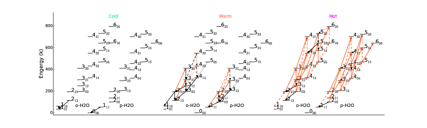
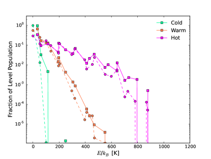
This finding is further illustrated in Fig. 3 where we show the most prominent lines predicted by our models for each ISM component. The black downward and red upward arrows denote emission and absorption, respectively. The relative line strength is coded in the line style with solid arrows indicating the strongest (70% of the maximum intensity, Imax), dash arrows medium (% of Imax) and dotted arrows weak lines with less that 10% of the maximum line intensity. Fig. 3 implies that the excitation of water is very sensitive to the underlying physical conditions. In Fig. 4 we present the partition functions (the fractional population of each level as a function of its energy) for each ISM component. The figure shows that only the first two or three levels (with energies below K) are populated in the cold ER, while water can efficiently be populated to levels with energies up to K in the warm gas component. Another useful feature to distinguish between the two ISM components is that the two ground-state lines seen in cold ER become invisible in the warm component. The different pattens shown in the Fig. 3 suggest that is powerful diagnostic tool to distinguish multiple ISM components with different physical conditions in galaxies.
4.3.2 Relation to the dust continuum and CO emission
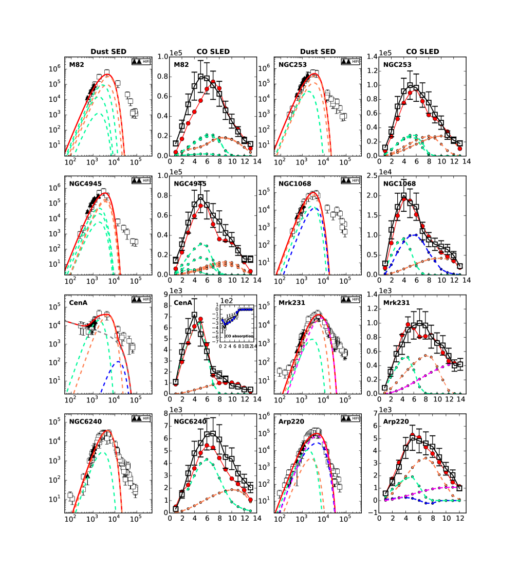
The two gas components also account for the major part of observed dust SED and CO SLED, although their generated dust SED and CO SLED are found to be very distinct. Fig. 19 presents the observed dust SED and CO SLED (in black points) as well as the results predicted from our best-fit models (red lines). Overall, most of IR luminosity is generated by the warm component (its dust SED peaks at FIR wavelength), while the dust continuum emission on the long wavelength Rayleigh-Jeans side arises mainly from the cold ER. The CO SLED of the warm component typically peaks at transitions and dominates the emission of middle/highJ CO lines () lines. The CO gas of the warm component almost approaches LTE in levels . On the other hand, the cold ER generates most of CO line emissions in the low CO transitions and its SLED peaks at . Our models on average recover around 70% of the observed dust continuum and CO line intensities. It is worth mentioning that we find a good match between the physical sizes of warm component (derived from model) and the starburst regions measured from high-resolution molecular gas or IR observations. This fact, in combination with its relatively high excitation of and CO, suggests that the warm component is associated with the nuclear starburst region in our sample galaxies. The cold ER, however, is likely associated with the more widespread quiescent ISM and may partly trace gas in the outer disks and spiral arms in some of our targets (e.g. in NGC253 and NGC4945).
4.3.3 H2O absorption
Another typical ISM component in our models is the bulk of the absorbing gas which normally locates in front of the warm component that dominates the FIR luminosity. Unlike the other two ISM components that exist in all galaxies, we have only detected absorption in ground-state and other low-excitation lines within five sources. The existence of the absorbing gas seems to depend on both the galaxy orientation and geometry structure. We find that the absorbing gas is more likely to be detected in the edge-on galaxies, as in the case of NGC 4945, NGC 253 and M82 in our sample. This is not surprising given that most of the cold material in the disk of a galaxy will not be located in front of the warm dust continuum if the galaxy is seen face-on (e.g, such as in NGC 1068). The absorbing gas is very likely partly associated with the cold ER given the similar physical parameters we find for the cold ER and the absorbing material in e.g. NGC4945 and NGC253. Furthermore the partition function of the cold gas (with a significant population of the first few energy levels of water only, see Fig. 4 left) naturally explains why absorption is usually only detected in the ground-state and the low-excitation lines. The medium-excitation lines from the background warm component can thereby pass through the cold ER almost without being absorbed. The profile of a resulting absorption line depends on how the cold ER is distributed relative to the warm component. If a large part of the warm component is covered by the cold ER, as suggested by our models for NGC 4945 and NGC 253, the absorption will appear to be very broad and deep. If only a small part of the warm component is covered, the absorption will be narrow and shallow as the case for M82.
Note that the absorbing gas does not always has to be associated with the cold ER. For example, the ground-state/low-excitation absorption detected in Arp 220 is found to arise from warm gas (possibly associated with molecular outflows driven by the nuclear activity) against the even warmer background radiation from the hot component.
4.3.4 Hot water in Mrk231 and Arp220
For the two most IR luminous sources in our sample, Mrk231 and Arp220, our models require another physical component contributing significantly to line intensities. This component is required to explain the high-excitation transitions exclusively detected towards both sources (e.g the p-H2O () line). The component contains a substantial amount of hot ( and K) and dense () gas with high column density (). The physical size of this hot component is found to be very compact ( pc). As we can see from the Fig. 3 (right), the high-excitation transitions from the hot gas are seen both in emission and absorption, most of which are not excited by the warm component. In the hot component, water can be populated to extremely high-excited levels with energies up to K (see Fig. 4). This is due to efficient collisional excitation in this gas phase and, more importantly, due to a combination of the strong IR emission associated with the hot gas and the large number of mid-IR water transitions which allow for efficient pumping of rotational levels to high energy states. A significant fraction of the continuum emission from the hot component, however, may be attenuated by foreground material at short wavelength (m) as the hot component is usually deeply buried in the galaxy nuclei (Downes & Eckart, 2007). Due to its small size, the hot gas component has only a small contribution to the low CO transitions but it becomes increasingly important for higher transitions and may dominate the CO SLED for CO lines with (see Fig. 19).
Finally, we find that the gas phase abundance of water varies from in the cold extended region, to in the warm component and jumps to in the hot gas due to the efficient release of H2O from dust grain into the gas phase at these high temperatures.
5. Discussion
5.1. Water Excitation in a Multi-Phase ISM
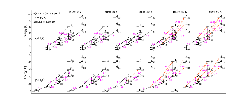
In order to explore the relative importance of collisions and IR pumping on the water excitation under typical conditions derived for our galaxy sample, we compute the water excitation in the warm gas component (, K, ) with varying the dust temperature from 0 to 50 K. The resulting emission and absorption lines from this calculation are shown in Fig. 5 while the underlying level populations are shown in form of Boltzmann diagrams in Fig. 6. From the first panel of Fig. 5 , which ignores the effect of IR pumping ( K), one can see that water can be excited by collision to levels with energies up to 250 - 350 K (250 K for p-H2O and 350 K for o-H2O). This picture does not change significantly as long as the dust temperature stays below K. Only when the dust temperatures reaches 40–50 K, IR pumping starts to play a dominant role by populating levels with K. The magenta numbers in Fig. 5 indicate the peak brightness temperature of each transition in the warm gas component (averaged over the surface of a single clump). From these numbers one can see that the line strength of transitions between levels K increases rapidly with dust temperature (e.g, o- () and p- ()). In contrast, line intensities for transitions with E K depend little on the dust temperature (e.g., o- ()) and some of them (e.g., the lines with E K) even decrease for an increasing dust temperature due to the increased continuum levels (e.g, o- ()).
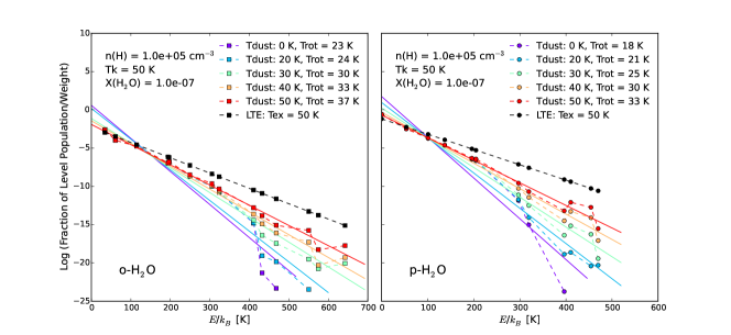
This behavior is more quantitatively shown in the Boltzmann diagrams in Fig. 6. The collisional excitation drives the o-H2O (p-H2O) populations with (100) K towards a Boltzmann distribution at the kinetic temperature (i.e. these levels are thermalised), and dominates the equilibrium population of the levels with (250) K for o-H2O (p-H2O) independent of the dust temperature. Note that this happens already at densities much below the critical density of the water lines () due to the high optical depth of these lines (see Equation A9 in Appendix). The population of levels with energies above 250 - 350 K, however, is almost exclusively determined by radiative pumping. Fig. 6 shows that the dust radiation field tends to drive the population of these levels (which are poorly populated by collisions) towards a Boltzmann distribution close to the dust temperature. When the dust temperature is about equal to the kinetic temperature (red points), the overall level population (from ground-state to most highly excited levels) can be fit well with a single rotational temperature (red solid line). However, we also notice that the rotational temperature can only rise to 50% - 70% of the dust temperature even at the highest dust temperature (). We attribute this effect to the dust optical depth, i.e., it is due to the modified blackbody shape, rather than a blackbody shape, of our dust radiation field.
The dust radiation energy is absorbed by the short-wavelength, far-IR transitions (see red upward arrows in Fig. 5) and then emitted by the long-wavelength, far-IR/submm high-excitation lines. Under the typical conditions in the warm gas derived for our galaxy sample, the most efficient pumping occurs at the strong //// lines (// lines for p-) through absorptions of far-IR photons at 75/66/58/40/79 m (90/67/46 m for p-), which greatly enhance the intensities of high-excitation //// (/ for p-) emission lines.
We have limited the discussion here to the typical warm environment derived for our galaxy sample. Whether a transition is excited mainly by IR pumping or collision in the general case is, however, very sensitive to the ambient ISM conditions. We show the Boltzmann diagrams for other cases in Fig. 21 in Appendix C. In summary our models suggest, that our observed low-excitation lines ( K) are collisionally excited, and most of the observed medium-excitation lines ( K) are also predominantly excited by collision. IR pumping starts to populate the medium-excitation transitions with for the typical dust fields derived in our sample and becomes increasingly important for higher transitions. For the high-excitation transitions with K, IR pumping is the dominant excitation channel even for the extreme ISM conditions derived for our hot gas in Arp 220 and Mrk 231.
5.2. SLED
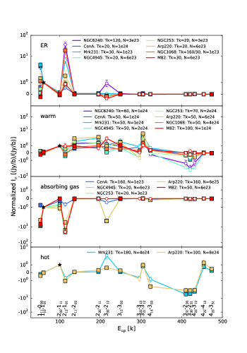
To investigate the spectral line energy distribution of within various ISM components and discuss the implications for the observed various line ratios, we present normalized SLEDs for our sample galaxies in Fig. 7. The solid squares in Fig. 7 indicate the observed values (for each velocity components as derived from the Gaussian decomposition), the open circles indicate the model predicted values for the lines without observations and the black star indicates the transition which has been used for the normalization. The kinetic temperature and the column density for each component are given in the plot legend, while the values for other parameters are presented in Table 4.
5.2.1 Elevated / ratios in the ER
The most remarkable feature in the first panel of Fig. 7, which shows normalized SLED for the extended region (note that ER for NGC 1068 also includes the component of outflow listed in Table 4), is that the / line ratios are strongly boosted in galaxies with high kinetic temperatures. The / line ratio varies from in galaxies with kinetic temperature around K (e.g., CenA, NGC 4945 and NGC 253), to the extreme large values () in galaxies with K, which are well known to harbor “shocked gas” (e.g., NGC 6240 and NGC 1068, Meijerink et al., 2013; Papadopoulos et al., 2014; Müller Sánchez et al., 2009; Wang et al., 2012, 2014). As such, we suggest that the / line ratio can be utilized as a good indicator of “shock condition” where gas is heated to high kinetic temperatures. The strong collisional excitation in shocks allows water to be populated above the ground states efficiently, and thereby strongly enhances the line intensity of .
5.2.2 Line ratios in the warm gas
The second panel in Fig. 7 presents normalized SLED for warm components of our galaxies. The line is one of the visible lines from the warm component that can be most easily excited by collisions (therefore least affected by radiative pumping), thereby the line ratios of other transitions to it can directly reflect the effect of radiative pumping. The first notable feature inferred from the plot is that the SLED seen in medium-excitation lines (from to ) appears to be nearly flat, with their emitted line intensities comparable within a factor of in our sample. This implies that the upper levels of these medium-excitation lines tend to approach statistical equilibrium in agreement with our findings in Sect. 5.1 and with the analysis by González-Alfonso et al. (2014).
However, all SLEDs show a peak at line, demonstrating that line has relatively stronger intensities since these medium-excitation lines have similar line frequencies ( GHz). The underlying reason is that the upper level is not only approximately thermalized by collisions (as the other lower levels), but it is also one of the levels that can be most easily excited by IR pumping (see Fig. 5 and Fig. 6). So the line usually exhibits higher excitation temperature. The line is found to be optically thinner () than the lower-excited medium-excitation lines () due to its required higher excitation energy. Therefore, the / line ratios are mostly sensitive to the total column density () and are enhanced in galaxies with higher . The / ratio exhibits the largest value () in Arp 220 which has highest (), moderate values () in galaxies with (e.g., NGC 4945, NGC 253, NGC 6240) and the smallest value () in M82 which has the lowest (). Yet, not all galaxies (e.g., CenA and NGC 1068) follow this trend, indicating that other parameters, such as the dust temperature as suggested by González-Alfonso et al. (2014), may also influence this ratio. A comparable trend is also seen in the line, which locates in a position of para-H2O energy diagram similar to that of the line in ortho-H2O energy diagram. The line also exhibits smaller line optical depth () and slightly higher excitation temperature than other para- medium-excitation lines. We have not found a strong variance of SLEDs over dust temperatures, possibly due to the small range of dust temperatures in our warm components or physically suggesting that radiative pumping does not play a dominant role in exciting these medium-excitation lines. Finally, we find that the lines that are most sensitive to collision ( and ) have larger intensities in galaxies with higher kinetic temperatures (e.g., M82).
5.2.3 The line ratios in the absorbing gas
The third panel in Fig. 7 shows the SLEDs for the absorbing gas of five galaxies in our sample, which are normalized to the absolute line intensity of the line. The first conclusion inferred from this plot is that the absorption is often observed only up to the line. This is because higher levels are usually not populated for this component. We further find that the SLED of absorbing gas is closely related to the dust SEDs ( and ) of both the background continuum source and the absorbing gas. If the dust continuum from the absorbing gas is negligible, then the ratios of absorption lines depend mainly on the flux ratios of background continuum sources at the line frequencies, as the low-excitation absorptions ( , ) are often found to be optically thick. We find that the galaxies whose absorbing gas contributes little to the dust continuum (e.g., K, in NGC 4945, M82 and NGC 253) have the / ratios around and the / ratios around , which are very close to the dust continuum 1113/557 GHz () and 1670/557 GHz () flux ratios of the background source (i.e., the warm component). However, once the dust continuum from the absorbing gas becomes significant (e.g., K, in Arp 220), the / and / line ratios will decrease as increasing column density of the absorbing gas (as the dust continuum and flux ratios are smaller at lower dust temperature and higher column density). In the cases where the absorption lines are optically thin (in this case, ), however, our modelling suggests that the / and / ratios can be significantly larger than the values estimated from the background dust continuum. We do not find optically-thin absorption lines in our work. The / and / ratios should be always larger than one, if the background continuum is a modified blackbody spectrum. Otherwise, it suggests that the background continuum may be a radio source with a power-law spectrum just as in the case of Cen A (see Appendix B for more details on Cen A). Thus, the ratios of absorption lines are able to provide valuable hints on the properties of background continuum sources even without spatially resolving the nuclear regions.
5.2.4 The H2O SLED of the hot gas
The last panel in Fig. 7 presents normalized SLED of hot component which has only been found in the ULIRGs in our sample (Arp 220 and Mrk 231). The SLED of hot component displays similar features with the warm component in medium-excitation lines but displays quite distinct behavior in high-excitation lines which show strong detections in both emission and absorption. Considering its high dust temperature and other extreme physical conditions, the hot component is possibly associated with a dusty toroid heated by an AGN (e.g., Downes & Eckart, 2007; Weiß et al., 2007).
5.3. Dependence of the water line intensities on the FIR continuum properties
5.3.1 The - correlation
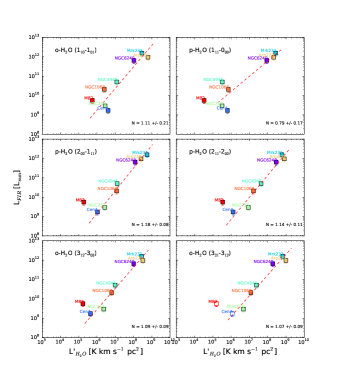
We present the correlations between (m) and for the two ground transitions and four medium-excitation lines in Fig. 8. Note that we adopted only the emission luminosity, rather than total line luminosity, for the two ground-state lines to avoid biases due to foreground absorption. Fig. 8 shows, that M82 deviates significantly from the overall correlations in particular for the medium-excitation lines. We attribute this finding to its lower water abundance (more details on M82 see Appendix B) and excluded M82 from our correlation analysis between and .
We find that all medium-excitation transitions show a tight nearly linear - correlation, which agrees well with the linear correlation found in larger galaxy sample observed with the SPIRE-FTS (Yang et al., 2013). As our model suggests that collision plays a significant role in exciting most of the medium-excitation transitions (see Fig. 5 and Fig. 6), this linear correlation is not simply a consequence of IR pumping as suggested by Yang et al. (2013). Our models show that the medium-excitation transitions probe the same physical regions of galaxies where most of FIR emission is generated (i.e., the warm component, see Section 4.3), suggesting that the observed correlations between FIR and the medium-excitation line is mostly driven by the sizes of the FIR and water emitting regions in these lines.
This view is also supported by the - correlations of the two ground-state lines which we present here for the first time. While the - correlation for o- () line has an approximately linear slope (), the p- () line shows a slope slightly below unity (). In addition, the correlations for ground-state lines have smaller Spearman rank correlation coefficients () compared with those for medium-excitation lines (), suggesting that the former are less correlated with compared with the latter. This is not surprising given that the ground-state lines are found to arise mostly from the cold extended regions of galaxies which contribute less to FIR luminosity.
5.3.2 Dependence on on the dust color
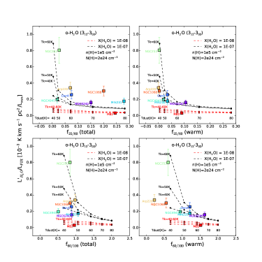
In order to investigate the variations of luminosity ratios () with , we have analyzed the correlation between and the IR colors ( and ) for the medium-excitation lines. All medium-excitation lines display a similar trend and we show as an example the relation for the o- () line in Fig. 9. The left column of Fig. 9 shows the observed ratios versus the observed total IR colors for our sample galaxies (with in the top row and in the bottom row), while the right column presents the observed versus the IR colors derived from the warm component only.
The first conclusion inferred from Fig. 9 is that we do not find a clear trend where the observed ratios vary with the observed total IR colors (for both and ), however, we find that the observed ratios decrease with the increasing values of IR colors estimated from the warm component only. The first fact could be due to the different physical origins of the observed ratios and IR colors. The former arises mainly from the warm component, while the observed and will be contaminated by other ISM components. The will be greatly enhanced if a strong AGN is present (e.g., Mrk231, NGC 1068 and Arp 220), while the will be decreased largely if the cold ER contributes significantly to the total IR luminosity. We can see from the right column of Fig. 9 that once the contamination in IR colors from other components is removed, ratios start to show a correlation with IR colors. Within a larger sample of galaxies that are detected by the SPIRE-FTS, however, a slight trend that the ratio decreases with increasing has been observed (Yang et al., 2013).
To further understand how the ratios vary with IR colors, we have modeled the relations between and IR colors for a set of warm components with variable dust temperatures, kinetic temperatures and water abundances but with a fixed gas density () and column density (). The dashed curves in Fig. 9 present the model results for the warm components. One can see that our model predicts a strong decrease of with increasing and (i.e., ), which is in very good correspondence with the trend seen in the warm component only.
We further find that the constant lines drop much faster at the low- end where most of our sample galaxies reside, while they decrease very little at the high- end. This is because the o- () line (along with the other medium-excitation lines in our work) is excited largely by collisions at low- (), and therefore its line intensity does not increase significantly with , but is greatly enhanced for increasing kinetic temperature. That is why NGC 253 stands out significantly in the plot, because it has a relatively high compared to its . At the high- end () where IR pumping becomes more important, the line intensity increases rapidly with and therefore its ratio to remains almost constant for increasing (i.e, IR colors), and it will show no dependence on . The ratio of o- () is found to be always larger than if , and decreases rapidly with decreasing water abundance.
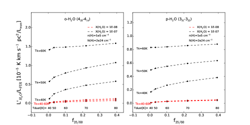
For the lines that are excited dominantly by IR pumping (such as the p- () and the o- () lines which have both not been observed in our work), our model predicts the ratios have a different dependence on the IR color than the lines mainly excited by collisions. As shown in Fig. 10 these lines do not show a decreasing but an increasing ratio for an increasing dust temperature. A similar trend is found by González-Alfonso et al. (2014), which suggests that the ratio is expected to decrease with increasing for all lines with K but increases with for the high-excitation lines with K. The modelling results shown in Fig. 9 and Fig. 10 imply that the observed correlation between and IR colors can be utilized as a diagnostic tool to distinguish between different excitation channels (i.e., collisional excitation and IR pumping) of lines. That is if the ratio is found to decrease with increasing IR color, then the line is possibly excited mainly by collision within the sample, otherwise the line may be excited dominantly by IR pumping.
5.4. The Implication of Line Profiles
Unlike the line profiles of other molecules (such as CO or HCN), the line shapes strongly depend on the involved energy levels. The absorption free medium-excitation transitions show line profiles in agreement with or slightly narrower than CO. Our model suggests that the medium-excitation lines stem from the same volume that gives rise to the FIR emission. This leads to a tight linear correlation between the luminosities of medium-excitation lines and FIR. We therefore conclude, that the medium-excitation lines are good probes to study the kinematics of the starburst/star-forming gas, e.g., they can serve as kinematic probes of the FIR emission region.
The line profiles of ground-state and low-excitation lines are found to differ from galaxy to galaxy. Some of these lines show pure absorption, while the others show pure emission or a mix of both. The emission of the ground-state lines often spans a larger velocity range than the medium-excitation transitions (e.g, NGC 4945, NGC 253 and NGC 1068), implying that the ground-state emission arises from a more extended physical region. This is most prominently seen in NGC 253 where the o- ground-state line is wider than the medium-excitation lines. The absorption line shapes and centroids depend on the dynamics of the foreground gas and its location related to the background continuum source. Although detailed kinematics of galaxies are not considered in our work, some important information can still be obtained by comparing the line profiles of with those of other species (e.g, CO, HF) and the high spacial-resolution CO observations.
We noticed that most absorption profiles have line shapes that deviate from pure Gaussian profiles and often show P-Cygni or inverse P-Cygni profiles indicative for non-circular motions driven by gas outflow or infall. For example, the absorption of NGC 4945 is better fitted by a broad Gaussian component centered close to the systemic velocity plus a redshifted (by ) narrower Gaussian component. The latter is possibly related to an infall of gas in the molecular ring or non-circular motion (for instance in a barred potential, van der Tak et al., 2016). The absorption of NGC 253 shows a P-Cygni profile which has also been observed in other gas species (e.g., HI and HF, Koribalski et al., 1995; Monje et al., 2014), and is likely connected to the molecular outflow observed in CO (Bolatto et al., 2013). By comparing the absorptions of M82 with high-resolution CO maps, Weiß et al. (2010) found the absorption of M82 only displays a good agreement with the CO profiles from a small region towards the galaxies center, implying that the absorption may arise from a small strip orthogonal to the molecular disk.
In the case of Arp 220 the ground-state (and low-excitation) absorption feature display a velocity dispersion which is much narrower than those of the medium-excitation emission lines ( compared to FWHM ), but in good agreement with the width of the high-excitation lines (). High-spatial resolution ALMA imaging by König et al. (2016) find that most of the high-excitation H2O line emission stems from the western nucleus which is also suspected to harbor a buried AGN (Downes & Eckart, 2007). The velocity centroid of the H2O absorption is consistent with that arising from the western source. It is therefore likely that the low-excitation absorption of Arp 220 arises within the compact western nucleus in a region that could be about the same size as the region where high-excitation lines are generated from.
The o- ground transition profile of Cen A is similar to those of low CO lines observed by Israel et al. (2014) showing a broad emission profile arising from the circumnuclear disk with a narrow absorption close to the systemic velocity against the compact nuclear source. In Cen A, the p- ground-state line shows an inverse P-Cygni profile, which could be a sign of infall (e.g., van der Tak et al., 2016).
Another interesting finding comes from a comparison between the line profiles of o- and p-. We find that parts of the o- and p- energy ladders are very similar, where the o- /// / levels correspond to the p- //// levels, respectively (see Fig. 1). Therefore, the p- ground-state (-) transition shows a good correspondence in the line shape to the o- () line rather than the o- (-) ground-state transition. This is also why the o- () and () lines have very similar shapes compared to the p- () and () lines, respectively, even though the upper levels of the former are around K higher than those of the latter.
6. Summary and Conclusion
Using HIFI on-board of Herschel we have obtained for the first time velocity-resolved spectra for a sample of nearby actively starforming galaxies. Our observations include the ground-state transitions of ortho and para H2O and cover transitions with E K. The main observational results from our spectroscopic survey are:
-
•
The spectra show a diversity of line shapes. The medium-excitation lines (E K) are always detected in emission. Their line profiles typically resemble those of CO indicating that water is widespread in the warm nuclear regions of active galaxies.
-
•
The line profiles of ground-state and low-excitation transitions (E K) often show a mix of emission and absorption. The emission features of these low-excitation lines usually display a wider velocity range than the medium-excitation lines, while the absorption features are often found to show more complex line profiles that differ from galaxy to galaxy.
We analyze the water excitation using the state of art, 3D non-LTE radiative transfer code ‘3D’. The main conclusions from the analysis are:
-
•
Multiple ISM components with different physical conditions are required to explain the observed line shapes and line intensities. We identify two ISM components which are present in all galaxies - an extended cold (T K) region (ER) and a warm (T K) component. The cold ER is only excited by collisions and has significant emission line intensities only in the ground-state and a few low-excitation lines. This gas component is also often responsible for the detected low-excitation absorption features seen in our targets. The warm component contributes almost all the emission of medium-excitation lines. For the two ultraluminous IR galaxies in our sample (Mrk 231 and Arp 220), our models suggest the presence of an even warmer gas component (hot gas) to explain the emission and absorption in the high-excitation H2O lines (E K).
-
•
The multiple ISM model also allows to explain the observed dust SED and CO SLED in our target galaxies. The cold ER contributes mainly to millimeter and submm dust continuum. The warm component dominates the total IR luminosity with its dust SED peaking at FIR regimes, suggesting that its generated medium-excitation H2O lines are excellent probes to study the kinematic of the FIR emitting regions. The middle/high () CO emission lines mainly arise from the warm component while the low CO transitions mainly come from the cold ER. The CO SLEDs of these two components peak at and , respectively. The hot component, if present, contributes large amounts of IR emission in MIR regimes (which however is usually attenuated by foreground dust) and has a significant effect on the CO SLED at levels with .
-
•
IR pumping dominates the excitation of high-excitation energy levels of water (with 250 - 350 K 500 - 700 K in warm component and K 1300 - 1600 K in hot component), and drive their level population towards a Boltzmann distribution close to the dust temperature. While collision dominates the excitation of low-excitation energy levels (with 100 - 150 K, 250 - 350 K and 600 - 800 K in cold, warm and hot components, respectively), and drive some low-excitation level population ( 150 - 200 K and 400 - 600 K in warm and hot components, respectively) towards a Boltzmann distribution at the kinetic gas temperature. Our observed low-excitation lines (with K) and most of the observed medium-excitation lines (with K) are excited dominantly by collision. IR pumping becomes more and more important in exciting our observed medium-excitation lines with K.
-
•
The gas phase abundance of varies from in the cold ER, to in the warm component and increases to in the hot component. Therefore, our results suggest that the water abundance is typically larger in the higher density and warmer regions.
Acknowledgements
We thank the anonymous referee for their carful reading of our manuscript and for their constructive comments and suggestions, which improved the paper. HIFI has been designed and built by a consortium of institutes and university departments from across Europe, Canada, and the United States under the leadership of SRON Netherlands Institute for Space Research, Groningen, The Netherlands, and with major contributions from Germany, France, and the US. Consortium members are: Canada: CSA, U.Waterloo; France: CESR, LAB, LERMA, IRAM; Germany: KOSMA, MPIfR, MPS; Ireland: NUI Maynooth; Italy: ASI, IFSI-INAF, Osservatorio Astrofisico di Arcetri – INAF; Netherlands: SRON, TUD; Poland: CAMK, CBK; Spain: Observatorio Astronmico Nacional (IGN), Centro de Astrobiologia (CSIC-INTA). Sweden: Chalmers University of Technology – MC2, RSS & GARD; Onsala Space Observatory; Swedish National Space Board, Stockholm University – Stockholm Observatory; Switzerland: ETH Zurich, FHNW; USA: Caltech, JPL, NHSC. LJ and YG acknowledge support by NSFC grants #11311130491, #11420101002 and CAS Key Research Program of Frontier Sciences B program #XDB09000000.
| Source | Line | FWHM | I | cont. | |
|---|---|---|---|---|---|
| M82 | o-H2O (110-101) | 86 2 | 122 6 | 320 0 | 13.6 3.4 (538 m) |
| -73 2 | 103 5 | 333 25 | |||
| 26 2 | 65 1 | -137 21 | |||
| p-H2O (111-000) | 86 2 | 122 6 | 153 | 85.0 13.6 (269 m) | |
| -73 2 | 103 5 | 140 | |||
| 26 2 | 65 1 | -869 34 | |||
| p-H2O (202-111) | 86 2 | 122 6 | 518 76 | 59.7 27.9 (303 m) | |
| -73 2 | 103 5 | 701 70 | |||
| 26 2 | 65 1 | 139 | |||
| p-H2O (211-202) | 86 2 | 122 6 | 458 54 | 33.2 5.0 (398 m) | |
| -73 2 | 103 5 | 584 41 | |||
| 26 2 | 65 1 | 83 | |||
| o-H2O (312-303) | 86 2 | 122 6 | 209 69 | 85.3 9.6 (273 m) | |
| -73 2 | 103 5 | 545 63 | |||
| 26 2 | 65 1 | 102 | |||
| p-H2O (422-331) | - | - | 53.0 8.5 (327 m) | ||
| NGC 253 | o-H2O (110-101) | 23 3 | 91 11 | 639 92 | 19.7 4.1 (538 m) |
| -60 3 | 96 11 | -106 40 | |||
| 80 3 | 94 9 | 1316 75 | |||
| p-H2O (111-000) | 23 3 | 91 11 | -2024 234 | 181.5 34.9 (269 m) | |
| -60 3 | 96 11 | -8548 160 | |||
| 80 3 | 94 9 | 3629 245 | |||
| o-H2O (212-101) | 23 3 | 91 11 | -4179 170 | 308.7 70.8 (179 m) | |
| -60 3 | 96 11 | -18579 214 | |||
| 80 3 | 94 9 | 905 | |||
| p-H2O (202-111) | 23 3 | 91 11 | 8001 454 | 114.5 26.4 (303 m) | |
| -60 3 | 96 11 | 4640 460 | |||
| 80 3 | 94 9 | 300 | |||
| p-H2O (211-202) | 23 3 | 91 11 | 6524 155 | 55.0 14.0 (398 m) | |
| -60 3 | 96 11 | 5927 161 | |||
| 80 3 | 94 9 | 268 | |||
| p-H2O (220-211) | 23 3 | 91 11 | 5496 181 | 224.4 30.3 (243 m) | |
| -60 3 | 96 11 | 4997 250 | |||
| 80 3 | 94 9 | 372 | |||
| o-H2O (303-212) | 23 3 | 91 11 | 4171 215 | 378.6 237.7 (174 m) | |
| -60 3 | 96 11 | 990 | |||
| 80 3 | 94 9 | 944 | |||
| o-H2O (312-303) | 23 3 | 91 11 | 5450 123 | 178.4 36.5 (273 m) | |
| -60 3 | 96 11 | 4692 151 | |||
| 80 3 | 94 9 | 302 | |||
| o-H2O (321-312) | 23 3 | 91 11 | 6316 382 | 201.3 32.0 (257 m) | |
| -60 3 | 96 11 | 8092 404 | |||
| 80 3 | 94 9 | 592 | |||
| p-H2O (422-331) | - | - | 98.0 24.3 (327 m) | ||
| NGC 4945 | o-H2O (110-101) | -112 3 | 98 7 | 1122 38 | 30.1 5.1 (538 m) |
| 48 3 | 136 10 | -2348 66 | |||
| 141 3 | 63 5 | 769 46 | |||
| p-H2O (111-000) | -112 3 | 98 7 | 295 | 237.4 36.6 (269 m) | |
| 48 3 | 136 10 | -25771 286 | |||
| 141 3 | 63 5 | 1579 138 | |||
| o-H2O (212-101) | -112 3 | 98 7 | 909 | 458.7 69.4 (179 m) | |
| 48 3 | 136 10 | -68706 291 | |||
| 141 3 | 63 5 | 729 | |||
| p-H2O (202-111) | -112 3 | 98 7 | 4301 87 | 173.9 24.8 (303 m) | |
| 48 3 | 136 10 | 2032 84 | |||
| 141 3 | 63 5 | 3890 60 | |||
| p-H2O (211-202) | -112 3 | 98 7 | 3430 207 | 85.3 15.4 (398 m) | |
| 48 3 | 136 10 | 3939 336 | |||
| 141 3 | 63 5 | 2285 198 | |||
| o-H2O (303-212) | -112 3 | 98 7 | 891 | 475.5 228.1 (174 m) | |
| 48 3 | 136 10 | -12823 231 | |||
| 141 3 | 63 5 | 714 | |||
| o-H2O (312-303) | -112 3 | 98 7 | 1548 120 | 240.8 39.2 (273 m) | |
| 48 3 | 136 10 | 2362 281 | |||
| 141 3 | 63 5 | 1842 169 | |||
| o-H2O (321-312) | -112 3 | 98 7 | 4135 304 | 277.9 31.5 (257 m) | |
| 48 3 | 136 10 | 5633 342 | |||
| 141 3 | 63 5 | 3658 255 | |||
| p-H2O (422-331) | - | - | 146.1 17.4 (327 m) | ||
| NGC 1068 | o-H2O (110-101) | -18 2 | 211 10 | 557 18 | 4.3 2.4 (538 m) |
| p-H2O (111-000) | -18 2 | 211 10 | 1552 72 | 18.9 10.9 (269 m) | |
| p-H2O (202-111) | -18 2 | 211 10 | 1554 94 | 17.1 11.4 (303 m) | |
| p-H2O (211-202) | -18 2 | 211 10 | 1264 74 | 8.7 3.4 (398 m) | |
| p-H2O (422-331) | - | - | 13.6 6.0 (327 m) | ||
| Cen A | o-H2O (110-101) | 0 2 | 235 11 | 682 58 | 10.1 2.6 (538 m) |
| 16 2 | 70 3 | -384 32 | |||
| p-H2O (111-000) | 0 2 | 235 11 | 384 138 | 16.9 7.0 (269 m) | |
| 16 2 | 70 3 | -358 75 | |||
| p-H2O (202-111) | 0 2 | 235 11 | 631 65 | 12.4 8.3 (303 m) | |
| 16 2 | 70 3 | 84 | |||
| p-H2O (211-202) | - | - | 11.6 5.8 (398 m) | ||
| p-H2O (220-211) | - | - | 17.1 11.4 (243 m) | ||
| o-H2O (312-303) | - | - | 15.0 6.6 (273 m) | ||
| o-H2O (321-312) | - | - | 18.4 12.2 (257 m) | ||
| p-H2O (422-331) | - | - | 11.6 7.7 (327 m) | ||
| Mrk 231 | o-H2O (110-101) | 50 2 | 211 10 | 66 77 | 0.4 0.3 (538 m) |
| p-H2O (111-000) | 50 2 | 211 10 | 362 44 | 3.3 2.2 (269 m) | |
| p-H2O (202-111) | 50 2 | 211 10 | 376 54 | 2.6 1.7 (303 m) | |
| p-H2O (211-202) | 50 2 | 211 10 | 588 67 | 1.1 0.7 (398 m) | |
| o-H2O (312-303) | 50 2 | 211 10 | 390 63 | 3.5 2.3 (273 m) | |
| p-H2O (422-331) | - | - | 2.1 1.4 (327 m) | ||
| Antennae | o-H2O (110-101) | - | - | 0.90 0.5 (538 m) | |
| p-H2O (111-000) | - | - | 4.65 3.0 (269 m) | ||
| p-H2O (202-111) | - | - | 1.96 1.2 (303 m) | ||
| p-H2O (211-202) | - | - | 1.71 1.5 (398 m) | ||
| o-H2O (312-303) | - | - | 3.00 2.0 (273 m) | ||
| p-H2O (422-331) | - | - | 2.25 1.9 (327 m) | ||
| NGC 6240 | o-H2O (110-101) | -10 2 | 282 14 | 175 33 | 0.5 0.3 (538 m) |
| p-H2O (111-000) | - | - | 4.5 3.0 (269 m) | ||
| p-H2O (202-111) | -10 2 | 282 14 | 660 116 | 4.6 3.0 (303 m) | |
| p-H2O (211-202) | -10 2 | 282 14 | 592 81 | 1.3 0.9 (398 m) | |
| o-H2O (312-303) | -10 2 | 282 14 | 253 53 | 3.1 2.1 (273 m) | |
| o-H2O (321-312) | - | - | 4.8 3.2 (257 m) | ||
| p-H2O (422-331) | - | - | 2.3 1.6 (327 m) | ||
| Arp 220 | o-H2O (110-101) | 52 5 | 412 32 | 812 133 | 2.5 1.6 (538 m) |
| 20 5 | 226 18 | -850 98 | |||
| 35 5 | 235 18 | 96 | |||
| p-H2O (111-000) | 52 5 | 412 32 | 449 | 24.3 14.3 (269 m) | |
| 20 5 | 226 18 | -3486 141 | |||
| 35 5 | 235 18 | 339 | |||
| p-H2O (202-111) | 52 5 | 412 32 | 3162 469 | 16.6 11.1 (303 m) | |
| 20 5 | 226 18 | -1369 477 | |||
| 35 5 | 235 18 | 288 | |||
| p-H2O (211-202) | 52 5 | 412 32 | 3481 91 | 7.9 4.2 (398 m) | |
| 20 5 | 226 18 | 132 | |||
| 35 5 | 235 18 | 134 | |||
| o-H2O (312-303) | 52 5 | 412 32 | 3021 156 | 23.5 11.3 (273 m) | |
| 20 5 | 226 18 | 232 | |||
| 35 5 | 235 18 | 237 | |||
| p-H2O (422-331) | 52 5 | 412 32 | 188 | 13.3 8.3 (327 m) | |
| 20 5 | 226 18 | 139 | |||
| 35 5 | 235 18 | 811 92 |
Note. — The errors of line centre () and line width () are not the real fitted errors, but the ranges by which the parameters are allowed to vary. We allow the position of each Gaussian component to change by ( in Arp 220) and the line width by ( in Arp 220). The upper limits to water intensities in Antennae are derived by adopting a FWHM from CO observation by Gao et al. (2001).
| (H) | |||||||||
|---|---|---|---|---|---|---|---|---|---|
| Source | Component | [pc] | [] | [K] | [K] | [] | [] | ||
| M82 | warm | -73 | 17 - 25 | ||||||
| warm | 86 | 17 - 25 | |||||||
| ER | -73, 86 | 60 - 90 | |||||||
| absorbing gas | 26 | ||||||||
| NGC 253 | warm | 23, -60 | 30 - 45 | ||||||
| ER | 80, -60 | 160 - 200 | |||||||
| absorbing gas | -60 | 50 - 60 | |||||||
| NGC 4945 | warm | -112, 48, 141 | 30 - 40 | 50 - 70 | 50 - 60 | ||||
| ER | -112, 141 | 120 - 180 | |||||||
| absorbing gas | 48 | 50 - 70 | |||||||
| NGC 1068 | warm | -18 | 70 - 100 | ||||||
| ER | -18 | 400 - 450 | |||||||
| outflow | -18 | 150 - 200 | |||||||
| Cen A | warm | 0 | 7 - 15 | ||||||
| ER | 0 | 70 - 100 | |||||||
| absorbing gas | 16 | pc | |||||||
| (case I) | |||||||||
| absorbing gas | 16 | pc | |||||||
| (case II) | |||||||||
| Mrk 231 | warm | 50 | 300 - 550 | ||||||
| ER | 50 | 1000 - 1500 | |||||||
| hot | 50 | 60 - 80 | |||||||
| NGC 6240 | warm | -10 | 250 - 350 | ||||||
| ER | -10 | 800 - 1000 | |||||||
| Arp 220 | warm | 52 | 120 - 150 | ||||||
| ER | 52 | 1000 - 1200 | |||||||
| absorbing gas | 20 | 70 - 100 | |||||||
| hot | 35 | 70 - 100 |
Note. — The physical parameters are given for a ISM component at a single velocity, and thereby the total size and gas mass of a ISM component are sum of the values derived for different velocities (). The continuum covering factor of the absorbing gas can be estimated as the total size of the absorbing gas compared to the total size of the warm background gas.
Appendix A A. The Methods of Line Modelling
A.1. A.1 Dust SED Model
The dust and gas are assumed to be coexistent in our model and their mass ratio is set to be the Galactic value of (e.g. Draine et al., 2007). Therefore, the frequency-dependent dust emission arising from a single ISM component with uniform physical properties can be calculated with a modified blackbody spectrum:
| (A1) |
where is the Planck function, is the total dust optical depth and is the solid angle of the ISM component determined by ( is the distance of galaxy). The dust optical depth was computed by:
| (A2) |
where is the total proton column density in , is the mass of a hydrogen nucleus in g and is the frequency dependence of the dust absorption coefficient in a form of in unit of (Priddey & McMahon, 2001). The dust emissivity index is set to 1.5.
The combination of dust SEDs from multiple ISM components depends on their physical distribution relative to each other. If they do not spatially overlap, the total dust SED is simply the sum of the individual dust SEDs from all ISM components. Otherwise, the absorption of dust continuum emission of the background component by the foreground dust needs to be taken into account:
| (A3) |
where is the solid angle of overlapping region and is the dust opacity of the foreground ISM component.
A.2. A.2 The 3D: the Extended Escape Probability Method
The level populations of molecular gas are determined by collisions and radiation through the equations of statistical equilibrium:
| (A4) |
where which is the total number of levels included, and are Einstein coefficients, and are collisional excitation () and de-excitation () rates. The collision rates of para- and ortho- with para- and ortho- (whose ortho-to-para ratio in thermal equilibrium is estimated by Equation (1) in Mumma et al. (1987)) have been taken from LAMDA database (Schoeier et al., 2005), which are originally calculated by Daniel et al. (2011).
The profile-averaged mean radiation intensity, , is given by:
| (A5) |
where is the source function, is the Planck function at the dust temperature and is the 2.7 K cosmic microwave background. The method has introduced two profile-averaged photon escape probabilities and . The is the probability that a photon escapes line absorption, and is the probability that a photon escapes dust absorption as well as line absorption and therefore contributes to the observed line emission by a distant observer. The first term of the right-hand side of the Equation A5 can be explained as the contribution of line photons, while the second term as the contribution of dust photons, and the third term as the amount of external radiation reaching the test point.
Under the Large Velocity Gradient (LVG) assumption and our assumption that the excitation of the molecular gas at a given point is only connected with the gas and dust of the same clump, the two escape probabilities and can be simplified into the following forms:
| (A6) |
| (A7) |
where is the line absorption coefficient, is the dust absorption coefficient with a form of in unit of (Priddey & McMahon, 2001), and are the line and dust optical depths, respectively, from the test point to the edge of the clump along a line of sight. The is calculated by a form of , where is the normalized absorption line profile contributed by turbulence and thermal speed of gas:
| (A8) |
where is the line rest frequency, is the Doppler velocity width in a form of ( is the turbulence velocity, is the Boltzmann constant, is the molecular weight and is the gas kinetic temperature). The turbulence velocity used to calculate the Doppler velocity width is estimated from molecular cloud linewidth-size scaling relations where a larger normalization value is adopted (i.e., ), since starburst galaxies are often reported to deviate the local classical molecular cloud scaling relations (Larson’s relations) (e.g., Swinbank et al., 2011; Kruijssen & Longmore, 2013). The grid size of clumps () are fixed to , but the corresponding physical sizes of grid cell and clump () are determined by the column density (H) of a clump and gas density n(H). In the absence of dust emission and absorption, we obtain the usual expression for the escape probability (e.g. Castor, 1970; Hollenbach & McKee, 1979). Finally, the critical density is calculated by:
| (A9) |
Due to the large Einstein coefficients, the critical densities of water lines are usually in the order of under the optically thin case () (Poelman et al., 2007).
Note that the angle dependence in the above equations is replaced by the summation over a fixed number of directions in our model, i.e., . The number of directions is arbitrary, but a 6-ray approximation is implemented, i.e., , to represent the six different orthogonal directions in a three-dimensional Cartesian grid. The line and dust optical depths ( and ) are calculated from the test point up to the edge of clump cube in each of six directions. Hence, the probability for a photon to escape is connected through all the grid points along six directions. Equation A4 - A7 constitute the core of our method to calculate level populations including dust radiation.
A.3. A.3 The Ray Tracing Approach
The ISM component, which is an ensemble of uniform clumps in a rectangular box, forms the basic unit in our ray tracing. We perform the ray tracing in a three-dimensional Cartesian grid, with axis along the line of sight. For each pixel (, ) in the projected surface (i.e., plane at ) , we calculate the line and dust continuum fluxes emerging from this pixel at different frequency channels by:
| (A10) |
| (A11) |
where labels all the grid cells in backward order along the ray, and indicates grid cells locating in front of the -th grid cell in backward order. The and indicate integrated line and dust optical depth of a single grid cell at (), respectively. And is the total number of grid cells along the direction, which is determined by the clump size () and number of clumps along the line of sight (i.e., = ). A simple physical interpretation of Equation A10 - A11 is that equals the amount of photons generated by molecular gas and dust at the grid cell (), and is the probability that a photon at grid cell () escapes both dust and line absorption along the direction.
We attribute the clumps inside an ISM component a random normal distributed global velocity field following the parameters derived by Gaussian decomposition of the H2O spectra. The final output of our ray tracing approach is a 3D line data cube, with the first two dimensions along the spatial -plane and the third dimension along frequency (or velocity). We then integrate the line cube along the -plane to derive a single global spectrum. In our ray tracing approach, the surface size (i.e., the area along the plane) of an ISM component is not important, since the modelled line intensity per unit area and the global line shape will not change with surface size as long as the given global velocity field can be fully sampled. We determine the physical size () of an ISM component by scaling the modelled line intensity per unit area to the observed value.
The spectra from multiple ISM components is simply the sum from individual ISM components if they do not spatially overlap. Otherwise, we need to integrate the emission through all the gas and dust of overlapped ISM components (i.e., in Equation. A10, is the total number of overlapped ISM components), in order to consider the line and dust absorption of the front ISM component against the background ISM component.
A.4. A.4 Select Best Models
In summary, our galaxy (nucleus) model is a combination of multiple ISM components. An ISM component is constrained by six parameters: , , , , and (H). The first five parameters constrain the excitation condition of the molecule ( and CO). The last parameter (H), together with the parameters (line centres and line widths) derived from Gaussian decomposition of our spectra, further determines the integrated line intensity and global line shape.
We model each velocity component of the spectra separately. For each velocity component, we derive the first and second ISM components by fitting the medium-excitation and ground-state/low-excitation emission lines, respectively. Additional ISM components are then added to fit the ground-state/low-excitation absorption lines and/or high-excitation lines where necessary. We first remove the underlying continuum and fit only the line intensities (negative integrated areas are fitted in the cases of absorption lines). The best-fit parameters for an ISM component are searched by minimizing the sum of chi-squared residuals. We then do a second pass to discard the models that significantly overestimate () the observed total continuum fluxes and CO () fluxes.
We utilize the ISM component dominating the FIR luminosity (normally the warm component derived by fitting medium-excitation lines) as the background continuum source of the ground-state/low-excitation absorptions. For each derived possible model of background warm component (or background hot component in the case of Arp 220), we search for the best-fit models of the absorption component by allowing its physical size to vary from zero to the maximum coverage. It’s worth mentioning that some models of the warm component (or hot component in the case of Arp 220) fail to produce satisfactory absorptions that match the observations, and we have discarded these models.
Since our models of individual ISM components are derived by fitting only certain transitions, they may significantly overestimate or underestimate line intensities of the other transitions. Therefore, we add up the modelled spectra from all the sets of ISM components at different velocities, and do a third pass by discriminate the combined models whose predicted global spectra show large discrepancies with the observations. The combined models with predicted global dust continuum or CO line intensities exceeding of the observed values were also excluded. The derived final parameters of our models are given in Table. 4.
Appendix B B. Detailed Models for Individual Galaxies
B.1. M82
M82 is a nearby, almost edge-on galaxy ( deg), notable for its spectacular bipolar outflow (e.g., Kamenetzky et al., 2012). High-resolution CO maps of the central kpc disk indicate that the molecular gas is largely concentrated in three areas: a north-east lobe, south-west lobe, and to a lesser extent, a central region (Weiß et al., 2001, 2010; Walter et al., 2002). Overall, M82 shows weaker line emission relative to CO. For example, the CO()/ ratio in M82 is much larger () compared to that of NGC 4945 () and NGC 253 (). Our models suggest that the faintness of H2O in M82 is mainly due to the lower abundance (see Table. 4). The blue-shifted and red-shifted emissions are associated with the south-western () and north-eastern () molecular lobes, respectively. Our model for M82 requires a warm and a more extended cold component to match the observed H2O line intensities, where the warm gas dominates the medium-excitation H2O lines, dust FIR continuum and high- () CO lines while the cold gas mainly contributes to the low-excitation , the long wavelength submm dust continuum and low/middle- () CO emission lines. The blue-shifted emission from the south-western lobe is stronger than the red-shifted emission from the north-eastern lobe. In our model this differences arise from the slightly elevated dust temperature in the south-western lobe compared to the north-eastern lobe ( K vs K). The absorption seen in ground-state lines occurs close to the systemic velocity () and does not have any correspondence to the emission features seen in medium-excitation H2O lines. This implies that the absorptions arise from a different region than the warm component, possibly from the front cold gas. As the absorption in M82 is observed to be much narrower and shallower than those in NGC 4945 and NGC 253, our model suggests that the cold gas in M82 covers only a small fraction of the continuum (). In a more detailed study of the H2O absorption in M82, Weiß et al. (2010) compared the absorption profile with high spatial resolution () CO observations. They find that the CO line profile is in very good agreement with the water absorption profile within only a small region at the galaxy center which associates with a strip orthogonal to the molecular disk of M82.
B.2. NGC253
NGC 253 is a nearby barred spiral galaxy with a compact nuclear starburst and a weak AGN in its center (Müller-Sánchez et al., 2010; Aalto et al., 2011). The nuclear starburst drives a 100 pc-scale molecular gas outflow/wind detected in CO (Mitsuishi et al., 2012; Bolatto et al., 2013). As in the case of M82 our model reveals that the medium-excitation emission lines and most of dust continuum arise from a warm ( K), dense () and compact ( pc) region which is very likely associated with the inner nuclear starburst disk. The line profiles of this warm gas component displays a double Gaussian and follows qualitatively the shape of the CO (3-2) line profile (see Fig. 2). It is, however, significantly narrower than the CO (3-2) emission profile and lacks emission at the terminal velocity of the CO spectrum. In contrast both ground transitions of o-H2O and p-H2O show emission significantly red wards () of the medium-excitation lines in good agreement with the shape of the red wing of the CO line profile. This demonstrates convincingly that the ground-state lines originate from a different physical volume than the medium-excitation lines and it is tempting to speculate that the H2O ground transitions are at least partly associated with the outflowing molecular material in NGC 253. This interpretation is also supported by the blue shifted () absorption seen in the p-H2O ground transition which forms together with the red shifted emission a P Cygni profile. We have modelled the blue and red line wings of the outflow using similar physical parameters resembling those found for the cold gas in NGC 4945. The two outflows generate almost equal emissions in ground-state o- () line (green dashed curves in Fig. 12). The reason for asymmetrical line shapes found in low-excitation lines of NGC 253 is simply due to their different spatial geometry with respect to the nuclear disk. That is the red-shifted outflow locates behind the nuclear disk, while the blue-shifted outflow resides in front of, and almost completely covers (), the nuclear disk (see Fig. 20), in agreement with the high spatial resolution CO maps from Bolatto et al. (2013). Therefore, the part of blue-shifted outflow locating right in front of the nuclear disk produces ground-state and low-excitation absorption lines, while the rest produces ground-state line emission. The absorption in o- () and o- () lines happen to compensate for the blue-shifted line emission, making these two lines partly invisible.
B.3. NGC4945
NGC4945 is a nearby, almost edge-on, disk galaxy. The central region of this galaxy contains an inclined nuclear starburst disk (Moorwood et al., 1996; Marconi et al., 2000; Chou et al., 2007) and a heavily enshrouded AGN (Iwasawa et al., 1993; Guainazzi et al., 2000; Pérez-Beaupuits et al., 2011). The central region is obscured by a strongly absorbing rotating circumnuclear star-forming ring seen nearly edge-on (Marconi et al., 2000; Spoon et al., 2003; Chou et al., 2007). Our modelling of NGC 4945 suggests that the strong emission seen in medium-excitation lines come from a dense (), warm ( K) region with a size of pc (this total size is sum of the sizes of three warm components at different velocities given by Table 4). The warm component is most likely associated with the nuclear starburst disk, whose size has been determined to be pc from high-resolution HST-NICMOS observations of the Pa line (Marconi et al., 2000) and CO interferometric maps (Chou et al., 2007). Since the warm nuclear disk material does not produce enough line emission in the low-excitation transitions, we added another ISM component to match these low-excitation emissions. We find the corresponding emission component is relatively cold ( K), less dense () and much more extended ( pc). By fitting the absorption features seen in ground-state/low-excitation lines, we obtain an absorption component with similar physical properties of the cold emission component except for its much smaller size ( pc). Thus, we speculate that the cold emission and absorption components arise from the same physical region which is very likely to be the surrounding molecular ring. In this picture, the ground-state emission seen at and arise from the edges of molecular ring, whose sight-lines do not intercept with the warm nuclear gas and are therefore free of absorption. The absorption feature at arises from the cold gas of the molecular ring which is located right in front of the warm nuclear disk. The warm nuclear disk is almost entirely covered by the cold gas of the molecular ring (i.e., ), given by the deep-to-bottom absorption seen at the velocity center. The terminal velocities in the low-excitation and medium-excitation spectra are almost identical (see Fig. 13), implying that the nucleus disk spans approximately the same range of velocities as the surround molecular ring. This interpretation is consistent with high spatial resolution CO maps which show that the rotation curve flattens beyond the radius of nuclear disk ( pc) (Chou et al., 2007). Note that the source size of the cold molecular ring (ER) given in Table 4 denotes the projected area at the two sides of the molecular ring rather than the real radius of the ring structure. The gas kinetic temperatures are found to be close to the dust temperatures within both the nucleus disk and molecular ring.
B.4. NGC1068
NGC 1068 is a nearby and bright Seyfert galaxy seen at an inclination angle of deg. Molecular gas (CO and HCN) observations towards its center have shown a central circumnuclear disk (CND) with a radius around pc (e.g., Krips et al., 2011; Spinoglio et al., 2012), and a star-forming ring/spiral at a radius of kpc (Tacconi et al., 1994; Schinnerer et al., 2000). As the brightest prototype Seyfert-2 AGN, NGC 1068 exhibits pronounced radio jets extending out to several kpc from the center (Gallimore et al., 2004; Krips et al., 2006). Following the above modelling approach, we utilized a warm component plus a cold component to match the medium-excitation and low-excitation emission lines, respectively. According to the derived physical parameters, the warm component is very likely associated with the CND, while the cold component should be at least partly related to the star-forming ring/spiral. In contrast to higher inclination galaxies in our sample, the low-excitation H2O lines in NGC 1068 do not show absorption, indicating that no cold gas is located in front of the warm CND. The model of above two components are able to fit most of lines very well, but fail to explain a large part of the o- () and middle- CO () line intensities which are very luminous in NGC 1068. Therefore, we added another component to match the remaining intensities of these lines. We find that this additional component contains a substantial amount of relatively low density (), low opacity () but very hot gas ( K) within a radius of pc. Therefore, we speculate that this gas is probably associated with the part of molecular gas in the CND which is shock heated to high kinetic temperatures as a consequence of an interaction between the radio jet and the CND (Krips et al., 2011). The strong interaction between the radio jet and the CND has been indicated by many recent observations: the CO and HCN line observations display a complex kinematic behaviour of the gas (e.g., Krips et al., 2011); MIR observations reveal hot and ionized gas following the orientation of the radio jet (e.g., Poncelet et al., 2008; Müller Sánchez et al., 2009); and X-ray observations show that clouds in many locations are strongly affected by shock heating (e.g., Wang et al., 2012). The strong collisional excitation of the shocked gas leads to enhanced emission of o- () line, and line ratios of CO middle to (e.g., CO ()/(), Wang et al., 2014) in NGC 1068. With this supplemented component of hot shocked gas, we are able to fit all the observed lines, dust SED and CO SLED very well.
B.5. Centaurus A, NGC5128
Cen A is the closest giant elliptical and a powerful radio galaxy (for a review, see Israel, 1998). Cen A exhibits a powerful and variable radio nucleus (Meisenheimer et al., 2007; Israel et al., 2008). Observations of molecular gas towards its central region ( kpc) has revealed several different prominent components: a nuclear disk ( pc) containing ionized and molecular gas, a compact circumnuclear molecular disk (CND, within the inner pc), as well as an even larger extended thin molecular disk (Espada et al., 2009; Espada, 2013; Israel et al., 2014; Salomé et al., 2016). According to our model, the ground-state emissions arise from a cold ( K), extended ( pc) region, which is likely related to dense gas in the CND or the outer molecular disk. Although we have only detected one line above ground-states, we are still able to roughly constrain physical parameters of warm component in Cen A by utilizing the upper limits of those undetected lines, together additional information from dust SED and CO SLED. The warm component in Cen A is found to be very compact (R pc), implying that only a small fraction of the gas is excited to high levels.
In order to model the absorption features seen in ground-state lines, we first adopted the dust continuum of warm component as the background. With this assumption we derived a cold ( K) absorbing gas component with extremely high optical depth ( ), which we consider as unrealistic as it would result in a dust SED inconsistent with the observation. We noticed that o- () line in Cen A has a almost comparable (or even a slightly higher) absorption depth compared with p- () line, which is very unusual as the ratios of their absorption intensities are much smaller () in all other cases. Considering these matters, the background source should be more likely the radio core rather than warm dust. Recent works found that at the lowest frequencies ( GHz) observed with SPIRE and HIFI, the continuum flux of Cen A is still completely dominated by the radio core (Israel et al., 2014, and Fig. 19). We adopted an index of -0.36 (, Meisenheimer et al., 2007) and a normalisation value of Jy (Israel et al., 2014) to model the radio power-law spectrum. As the radio core is unresolved even at very high spatial resolution ( or pc, Israel, 1998; Espada et al., 2009), we adopt different values from 0.01 pc to 10 pc for its physical size (). Our models suggest that the absorptions arise from either less dense () but high kinetic temperature ( K) gas, or relatively denser () but cold ( K) gas. The former may associate with shocked gas around the base of the radio jet (Ott et al., 2013), while the latter could be related to cold dense gas in the circumnuclear molecular disk or the outer molecular gas disk. Our model can also explain the absorptions detected in low CO lines (see the top subplot in panel of Cen A of Fig. 19, where the observed CO data points are from Israel et al. (2014)). We obtain same model results for pc, however, no satisfactory solutions can be found any more if the radio core becomes larger than a few pc.
B.6. Mrk 231
Mrk 231 is the most luminous infrared galaxy in the local universe, with (Sanders et al., 2003). Multi-wavelength observations reveal a QSO-like nucleus (e.g., Soifer et al., 2000; Gallagher et al., 2002) and a compact starburst disk (e.g., Carilli et al., 1998; Tacconi et al., 2002), embedded in a more extended ( kpc scale) diffuse disk (Taylor et al., 1999). Our favored model for Mrk 231 consists of a cold ( K), extended ( pc) diffuse halo, a warm ( K) starburst disk of radius pc and a highly obscured, compact ( pc) hot ( K) dense ( ) component. Our derived sizes are in good agreements with iterferometric imaging of CO() and () lines, which shows that a starburst disk with pc (Downes & Solomon, 1998) embedding in a kpc extended diffuse disk (Taylor et al., 1999). Unlike normal LIRGs of our sample, Mrk 231 shows intense high-excitation features (with K) in both emission and absorption, which can not be explained by the warm component. Our model reveals these high-excitation lines emerge from a very compact component with extremely high dust temperature and gas density, which is most likely related to the AGN dominated region. The contributions of hot component to line intensities are denoted by magenta dashed curves in Fig. 16.
The observed and modelled dust SED and CO SLED of Mrk 231 are presented in Fig. 19. As one can see from the figure, the bulk of far-IR continuum arises from the warm disk (with ), while large amounts of mid-IR continuum fluxes arise from the hot component (with and ). The hot component of Mrk 231 accounts for about of the total infrared luminosity, but contains only of the total dust mass. Note that the hot component should be deeply buried into the warm starburst disk and halo. Otherwise, it will severely overshine dust SED in mid-IR wavelength regime. In our model, the mid-IR infrared emission from the hot component is attenuated by foreground dust with . The CO SLED of Mrk 231 displays an approximately flat distribution over rotational ladders above , due to the strong high- CO emissions from the hot component. Finally, our model for Mrk 231 is broadly consistent with the model derived by González-Alfonso et al. (2010).
B.7. The Antennae Galaxies - NGC4038/NGC4039
The Antennae is an early-stage merger between two gas-rich spiral galaxies NGC 4038 and NGC 4039 (Schirm et al., 2014). Its majority of molecular gas and star formation is occurring within two nuclei and the overlap region (e.g., Gao et al., 2001; Schirm et al., 2014, 2016). Our HIFI single-pointing observations were positioned at the overlap region, which is the strongest continuum source of the Antennae. We do not have any detections within this region, which we suspect is due to its low mass of dense gas. If assuming the overlap region has a warm component that is similar to those found in other galaxies, we estimate its physical size to be around pc and dense gas mass around a few . The dust SED fitting predicts that its dust temperature is around K and dust mass around . Our derived low mass of warm dense gas is consistent with recent studies based on SPIRE-FTS CO observations using a non-LTE analysis (Schirm et al., 2014) and high angular-resolution observations of dense molecular gas (HCN and HNC) with ALMA (Schirm et al., 2016), which showed that the fraction of molecular gas in dense and warm phase in the Antennae is only around .
B.8. NGC6240
NGC 6240 is an early-stage merger hosting two nuclei that are separated by (Beswick et al., 2001). CO observations reveal that most of molecular gas in NGC 6240 is located in the overlap region of the two nuclei (e.g., Iono et al., 2007; Engel et al., 2010; Feruglio et al., 2013b, a). We utilized a warm component to model medium-excitation emissions (which is likely associated with the gas concentration between the two nuclei), and an extended low-excitation component (i.e., ER) to account for ground-state emissions. The latter is likely associated with the large-scale ( kpc) gas distribution detected in CO (Downes & Solomon, 1998). While the warm gas component in NGC 6240 shows similar physical properties with those derived for other galaxies, the low-excitation gas is inconsistent with the parameters found in other systems but exhibits a much higher kinetic temperature ( K, see Table. 4). This high kinetic temperature is required to match the exceptionally high line-to-continuum ratios () found in ground-state and low- CO () lines. The line-to-continuum ratio () of ground-state transitions for NGC 6240 is around , which is significantly higher than the value found e.g. for Mrk 231 (). The high line-to-continuum ratios of CO lines has been investigated in several recent publications and have been attributed to galaxy-wide shocks due to the advance merger state of NGC 6240 (e.g., Meijerink et al., 2013; Papadopoulos et al., 2014). This picture also explains the strong () S(1) emission at 2.12 m (Goldader et al., 1995), the spectacular butterfly-shaped emission-line nebula seen in HST H images (Gerssen et al., 2004) and Chandra X-ray image (Feruglio et al., 2013a), and the massive molecular outflow detected by the high-resolution interferometry CO maps (Feruglio et al., 2013b) and HCN/CS maps (Scoville et al., 2015). Our model with high kinetic temperatures but normal dust temperatures gives further support to this picture.
Note that we use the integrated fluxes from Herschel/SPIRE for p- () and o- () lines since they are not detected by our HIFI observations. Herschel/PACS observations show that high-excitation lines of NGC 6240 are much weaker than those of Mrk 231 or Arp 220. This suggests that a significant hot component, similar to the one in Mrk 231 or Arp 220, may not exist in NGC 6240. This is in agreement with our dust SED fitting which suggests that the size of such a hot component, if it exists, can not be larger than pc.
B.9. Arp 220
Arp 220 is the nearest ultra-luminous infrared galaxy. It is a late-stage merger with two counter-rotating disks separated by roughly (or pc), orbiting within an extended kpc-scale molecular gas disk (e.g. Scoville et al., 1997; Downes & Solomon, 1998). A highly dust-obscured AGN in the western nucleus of Arp 220 is suggested by mounting evidence (e.g. Downes & Eckart, 2007). A large reservoir of molecular gas has been observed to be concentrated in both nuclear disks ( pc from CO(6–5) map) (Scoville et al., 1997; Tunnard et al., 2015; Rangwala et al., 2015). High-resolution ALMA imaging of dense gas (CO(6–5), HCN, CS) have shown, that the two nuclei have almost the same line centroids and velocity dispersions (with velocity offset only being ) (Scoville et al., 2015; Rangwala et al., 2015). Thus, we can not kinematically separate the two nuclei in our spectra and thereby we model the two nuclei together as a single region. The predicted size and line intensities of each nucleus, therefore, are half of our modelled values, if they are assumed to be equal. We note that recent high-spatial resolution observations of H2O with ALMA, however, showed that 2/3 of the high-excitation water emission is emitted by the western nucleus (König et al., 2016). It is worth noting that strong self-absorption has been detected at the centers of both nuclei, where CO , HCN, and CS lines show double peaked velocity profiles in both nuclei (Scoville et al., 2015; Rangwala et al., 2015; Wang et al., 2016). So it is possible that the double peaked line shapes seen in our spectra are also due to self-absorption. We thereby utilized a broad Gaussian emission plus a narrow absorption to fit the double peaked lines.
We first model the medium-excitation and high-excitation lines of Arp 220. We found the medium-excitation lines come from a warm ( K) region (, pc), which is very likely to associate with the outer starburst regions of two nuclear disks. The high-excitation lines arise from a very compact ( pc), hot ( K) region whose column density is extremely high (). The hot component is very likely associated with the compact AGN- or starburst-dominated region at the nuclear center. To match the absorptions seen in ground-state and low-excitation lines, we add a third component in front of the hot component. The gas absorber is located in front of the hot component rather than the warm component because it is the hot component which dominates dust continuum emission and displays a velocity dispersion () comparable to the line width of the absorptions (). Our model reveals that the ground-state/low-excitation absorptions arise from an ISM component with warm dust temperature ( K), high gas temperature ( K) and large column density (), whose line intensities are denoted by blue dashed curves in Fig. 18. The absorption component is not likely to arise from the part of warm disk, given by its very distinct physical properties. Considering its high gas temperature, the absorption component is very likely to associate with massive outflows driving from the nuclei. The molecular outflows have been suggested by many molecular gas (like , and ) observations, which show P Cygni absorption line profiles in both nuclei (Sakamoto et al., 2009; Tunnard et al., 2015). The last component required to account for the broad ground-state emissions of Arp 220, is a kpc-size ( pc) molecular disk with large amounts of cold ( K), less dense () gas.
Our model for Arp 220 is also capable of explaining the observed dust SED and CO SLED (see Fig. 19). The massive kpc-size molecular disk, where the two nuclei are embedded in, contributes most of submm continuum flux and low () CO emissions (green lines). The warm component (i.e., the outer starburst regions of two nuclei) barely contributes to total dust continuum, but it produces the major part of dense gas emissions such as medium-excitation and CO lines (orange lines). The hot component and its massive molecular outflow dominate dust SED in FIR/MIR regime, whose size ( pc) matches the observed dust continuum size ( pc) well. We therefore predict that dust continuum comes from a more compact region than dense gas emission, which has been confirmed by several observations (e.g., Rangwala et al., 2015). Our model also suggests strong self-absorptions in CO lines by the molecular outflow (blue points in Fig. 19). As the absorption intensities (blue points) are comparable to (or even larger than) CO emissions from the hot component (magenta points), CO lines should be close to (or even go below) zero continuum level, at the center region where hot component and its molecular outflow reside in. This picture corresponds well with high resolution ALMA CO (6-5) observation which displays a double-peaked line profile at the centers of both nuclei but shows blue/red line peaks further outside (Rangwala et al., 2015). The high () CO lines, however, arise mainly from the hot component and they shine through molecular outflows without absorptions. A schematic representation of our model for Arp 220 is given in Fig. 20. Finally, we compare our model of Arp 220 with that in González-Alfonso et al. (2004, 2012). Overall, our model predicts a roughly similar hot component, but results in a denser, more compact and opaque warm component. Our model also requires a molecular outflow rather than an extended halo (González-Alfonso et al., 2004, 2012) to match the absorptions seen in low-excitation lines.
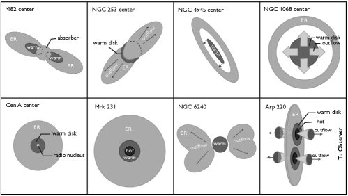
Appendix C C. Water Excitation Under Different Physical Conditions
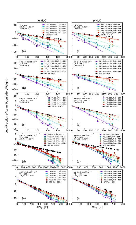
We present the level populations of water under different physical conditions in Fig. 21. The subplot (a - b) in Fig. 21 show that water gas is sub-thermally excited when gas density is not exceeding and water abundance is smaller than . The subplot (c) shows that the excitation temperature of water increase with increasing kinetic temperatures since the low/moderate-excited levels are mainly collisionally excited under the physical conditions of and . Once the gas density, kinetic temperature and water abundance increase to extremely large values (, K and ) as the case of hot component found in ULIRGs, the water level population can be thermally excited up to K as shown in subplot (d). When the dust temperature is larger than the kinetic temperature, the thermalized levels start to be overpopulated by IR pumping, i.e., IR pumping starts to play a role in exciting the thermalized lines. For example, the level populations of o- with K (and K for p-) in the warm component will not vary with the dust temperature if (see Fig. 5). However, once , more and more water will be populated within these levels with increasing dust temperature (see subplot (e) in Fig. 21).
References
- Aalto et al. (2011) Aalto, S., Costagliola, F., van der Tak, F., & Meijerink, R. 2011, A&A, 527, A69
- Aalto et al. (2015) Aalto, S. et al. 2015, A&A, 584, A42
- Bergin et al. (2003) Bergin, E. A., Kaufman, M. J., Melnick, G. J., Snell, R. L., & Howe, J. E. 2003, ApJ, 582, 830
- Bergin et al. (1998) Bergin, E. A., Melnick, G. J., & Neufeld, D. A. 1998, ApJ, 499, 777
- Bergin et al. (2000) Bergin, E. A. et al. 2000, ApJ, 539, L129
- Beswick et al. (2001) Beswick, R. J., Pedlar, A., Mundell, C. G., & Gallimore, J. F. 2001, MNRAS, 325, 151
- Bialy & Sternberg (2015) Bialy, S., & Sternberg, A. 2015, MNRAS, 450, 4424
- Bolatto et al. (2013) Bolatto, A. D. et al. 2013, Nature, 499, 450
- Carilli et al. (1998) Carilli, C. L., Wrobel, J. M., & Ulvestad, J. S. 1998, AJ, 115, 928
- Caselli et al. (2010) Caselli, P. et al. 2010, A&A, 521, L29
- Castor (1970) Castor, J. I. 1970, MNRAS, 149, 111
- Cernicharo et al. (2006a) Cernicharo, J. et al. 2006a, ApJ, 649, L33
- Cernicharo et al. (2006b) Cernicharo, J., Goicoechea, J. R., Pardo, J. R., & Asensio-Ramos, A. 2006b, ApJ, 642, 940
- Chou et al. (2007) Chou, R. C. Y. et al. 2007, ApJ, 670, 116
- Combes et al. (2012) Combes, F. et al. 2012, A&A, 538, L4
- Combes & Wiklind (1997) Combes, F., & Wiklind, T. 1997, ApJ, 486, L79
- Daniel et al. (2011) Daniel, F., Dubernet, M.-L., & Grosjean, A. 2011, A&A, 536, A76
- Downes & Eckart (2007) Downes, D., & Eckart, A. 2007, A&A, 468, L57
- Downes & Solomon (1998) Downes, D., & Solomon, P. M. 1998, ApJ, 507, 615
- Downes et al. (1993) Downes, D., Solomon, P. M., & Radford, S. J. E. 1993, ApJ, 414, L13
- Draine et al. (2007) Draine, B. T. et al. 2007, ApJ, 663, 866
- Elmegreen et al. (1980) Elmegreen, B. G., Morris, M., & Elmegreen, D. M. 1980, ApJ, 240, 455
- Emprechtinger et al. (2012) Emprechtinger, M., Monje, R. R., van der Tak, F. F. S., van der Wiel, M. H. D., Lis, D. C., Neufeld, D., Phillips, T. G., & Ceccarelli, C. 2012, ApJ, 756, 136
- Engel et al. (2010) Engel, H. et al. 2010, A&A, 524, A56
- Espada (2013) Espada, D. 2013, in Astronomical Society of the Pacific Conference Series, Vol. 476, New Trends in Radio Astronomy in the ALMA Era: The 30th Anniversary of Nobeyama Radio Observatory, ed. R. Kawabe, N. Kuno, & S. Yamamoto, 69
- Espada et al. (2009) Espada, D. et al. 2009, ApJ, 695, 116
- Feruglio et al. (2013a) Feruglio, C. et al. 2013a, A&A, 549, A51
- Feruglio et al. (2013b) Feruglio, C., Fiore, F., Piconcelli, E., Cicone, C., Maiolino, R., Davies, R., & Sturm, E. 2013b, A&A, 558, A87
- Fischer et al. (1999) Fischer, J. et al. 1999, Ap&SS, 266, 91
- France et al. (2014) France, K., Herczeg, G. J., McJunkin, M., & Penton, S. V. 2014, ApJ, 794, 160
- Gallagher et al. (2002) Gallagher, S. C., Brandt, W. N., Chartas, G., Garmire, G. P., & Sambruna, R. M. 2002, ApJ, 569, 655
- Gallimore et al. (2004) Gallimore, J. F., Baum, S. A., & O’Dea, C. P. 2004, ApJ, 613, 794
- Gao et al. (2001) Gao, Y., Lo, K. Y., Lee, S.-W., & Lee, T.-H. 2001, ApJ, 548, 172
- Gerssen et al. (2004) Gerssen, J., van der Marel, R. P., Axon, D., Mihos, J. C., Hernquist, L., & Barnes, J. E. 2004, AJ, 127, 75
- Goldader et al. (1995) Goldader, J. D., Joseph, R. D., Doyon, R., & Sanders, D. B. 1995, ApJ, 444, 97
- González-Alfonso et al. (2014) González-Alfonso, E., Fischer, J., Aalto, S., & Falstad, N. 2014, A&A, 567, A91
- González-Alfonso et al. (2013) González-Alfonso, E. et al. 2013, A&A, 550, A25
- González-Alfonso et al. (2012) —. 2012, A&A, 541, A4
- González-Alfonso et al. (2010) —. 2010, A&A, 518, L43
- González-Alfonso et al. (2004) González-Alfonso, E., Smith, H. A., Fischer, J., & Cernicharo, J. 2004, ApJ, 613, 247
- Greve et al. (2014) Greve, T. R. et al. 2014, ApJ, 794, 142
- Guainazzi et al. (2000) Guainazzi, M., Matt, G., Brandt, W. N., Antonelli, L. A., Barr, P., & Bassani, L. 2000, A&A, 356, 463
- Helou et al. (1985) Helou, G., Soifer, B. T., & Rowan-Robinson, M. 1985, ApJ, 298, L7
- Hollenbach & McKee (1979) Hollenbach, D., & McKee, C. F. 1979, ApJS, 41, 555
- Iono et al. (2007) Iono, D. et al. 2007, ApJ, 659, 283
- Israel (1998) Israel, F. P. 1998, A&A Rev., 8, 237
- Israel et al. (2014) Israel, F. P. et al. 2014, A&A, 562, A96
- Israel et al. (2008) Israel, F. P., Raban, D., Booth, R. S., & Rantakyrö, F. T. 2008, A&A, 483, 741
- Iwasawa et al. (1993) Iwasawa, K., Koyama, K., Awaki, H., Kunieda, H., Makishima, K., Tsuru, T., Ohashi, T., & Nakai, N. 1993, ApJ, 409, 155
- Kamenetzky et al. (2012) Kamenetzky, J. et al. 2012, ApJ, 753, 70
- König et al. (2016) König, S. et al. 2016, ArXiv e-prints
- Koribalski et al. (1995) Koribalski, B., Whiteoak, J. B., & Houghton, S. 1995, PASA, 12, 20
- Krips et al. (2006) Krips, M., Eckart, A., Neri, R., Schödel, R., Leon, S., Downes, D., García-Burillo, S., & Combes, F. 2006, A&A, 446, 113
- Krips et al. (2011) Krips, M. et al. 2011, ApJ, 736, 37
- Kruijssen & Longmore (2013) Kruijssen, J. M. D., & Longmore, S. N. 2013, MNRAS, 435, 2598
- Loenen et al. (2010) Loenen, A. F. et al. 2010, A&A, 521, L2
- Marconi et al. (2000) Marconi, A., Oliva, E., van der Werf, P. P., Maiolino, R., Schreier, E. J., Macchetto, F., & Moorwood, A. F. M. 2000, A&A, 357, 24
- Markwardt (2009) Markwardt, C. B. 2009, in Astronomical Society of the Pacific Conference Series, Vol. 411, Astronomical Data Analysis Software and Systems XVIII, ed. D. A. Bohlender, D. Durand, & P. Dowler, 251
- Meijerink et al. (2013) Meijerink, R. et al. 2013, ApJ, 762, L16
- Meisenheimer et al. (2007) Meisenheimer, K. et al. 2007, A&A, 471, 453
- Melnick et al. (2000) Melnick, G. J. et al. 2000, ApJ, 539, L77
- Menten et al. (2008) Menten, K. M., Lundgren, A., Belloche, A., Thorwirth, S., & Reid, M. J. 2008, A&A, 477, 185
- Mitsuishi et al. (2012) Mitsuishi, I., Yamasaki, N. Y., & Takei, Y. 2012, in American Institute of Physics Conference Series, Vol. 1427, American Institute of Physics Conference Series, ed. R. Petre, K. Mitsuda, & L. Angelini, 135–137
- Monje et al. (2014) Monje, R. R., Lord, S., Falgarone, E., Lis, D. C., Neufeld, D. A., Phillips, T. G., & Güsten, R. 2014, ApJ, 785, 22
- Moorwood et al. (1996) Moorwood, A. F. M., van der Werf, P. P., Kotilainen, J. K., Marconi, A., & Oliva, E. 1996, A&A, 308, L1
- Müller Sánchez et al. (2009) Müller Sánchez, F., Davies, R. I., Genzel, R., Tacconi, L. J., Eisenhauer, F., Hicks, E. K. S., Friedrich, S., & Sternberg, A. 2009, ApJ, 691, 749
- Müller-Sánchez et al. (2010) Müller-Sánchez, F., González-Martín, O., Fernández-Ontiveros, J. A., Acosta-Pulido, J. A., & Prieto, M. A. 2010, ApJ, 716, 1166
- Mumma et al. (1987) Mumma, M. J., Weaver, H. A., & Larson, H. P. 1987, A&A, 187, 419
- Omont et al. (2011) Omont, A. et al. 2011, A&A, 530, L3
- Omont et al. (2013) —. 2013, A&A, 551, A115
- Ott et al. (2013) Ott, J. et al. 2013, ApJ, 771, L41
- Panuzzo et al. (2010) Panuzzo, P. et al. 2010, A&A, 518, L37
- Papadopoulos et al. (2012) Papadopoulos, P. P., van der Werf, P. P., Xilouris, E. M., Isaak, K. G., Gao, Y., & Mühle, S. 2012, MNRAS, 426, 2601
- Papadopoulos et al. (2014) Papadopoulos, P. P. et al. 2014, ApJ, 788, 153
- Pérez-Beaupuits et al. (2011) Pérez-Beaupuits, J. P., Wada, K., & Spaans, M. 2011, ApJ, 730, 48
- Poelman & Spaans (2005) Poelman, D. R., & Spaans, M. 2005, A&A, 440, 559
- Poelman & Spaans (2006) —. 2006, A&A, 453, 615
- Poelman et al. (2007) Poelman, D. R., Spaans, M., & Tielens, A. G. G. M. 2007, A&A, 464, 1023
- Poelman & van der Tak (2007) Poelman, D. R., & van der Tak, F. F. S. 2007, A&A, 475, 949
- Poncelet et al. (2008) Poncelet, A., Sol, H., & Perrin, G. 2008, A&A, 481, 305
- Priddey & McMahon (2001) Priddey, R. S., & McMahon, R. G. 2001, MNRAS, 324, L17
- Rangwala et al. (2011) Rangwala, N. et al. 2011, ApJ, 743, 94
- Rangwala et al. (2015) Rangwala, N., Maloney, P. R., Wilson, C. D., Glenn, J., Kamenetzky, J., & Spinoglio, L. 2015, ApJ, 806, 17
- Rosenberg et al. (2014) Rosenberg, M. J. F., Kazandjian, M. V., van der Werf, P. P., Israel, F. P., Meijerink, R., Weiß, A., Requena-Torres, M. A., & Güsten, R. 2014, A&A, 564, A126
- Sakamoto et al. (2009) Sakamoto, K. et al. 2009, ApJ, 700, L104
- Salomé et al. (2016) Salomé, Q., Salomé, P., Combes, F., Hamer, S., & Heywood, I. 2016, A&A, 586, A45
- Sanders et al. (2003) Sanders, D. B., Mazzarella, J. M., Kim, D.-C., Surace, J. A., & Soifer, B. T. 2003, AJ, 126, 1607
- Schinnerer et al. (2000) Schinnerer, E., Eckart, A., Tacconi, L. J., Genzel, R., & Downes, D. 2000, ApJ, 533, 850
- Schirm et al. (2016) Schirm, M. R. P., Wilson, C. D., Madden, S. C., & Clements, D. L. 2016, ApJ, 823, 87
- Schirm et al. (2014) Schirm, M. R. P. et al. 2014, ApJ, 781, 101
- Schoeier et al. (2005) Schoeier, F. L., van der Tak, F. F. S., van Dishoeck, E. F., & Black, J. H. 2005, VizieR Online Data Catalog, 343
- Scoville et al. (2015) Scoville, N. et al. 2015, ApJ, 800, 70
- Scoville et al. (1997) Scoville, N. Z., Yun, M. S., & Bryant, P. M. 1997, ApJ, 484, 702
- Soifer et al. (2000) Soifer, B. T. et al. 2000, AJ, 119, 509
- Spinoglio et al. (2012) Spinoglio, L. et al. 2012, ApJ, 758, 108
- Spoon et al. (2003) Spoon, H. W. W., Moorwood, A. F. M., Pontoppidan, K. M., Cami, J., Kregel, M., Lutz, D., & Tielens, A. G. G. M. 2003, A&A, 402, 499
- Swinbank et al. (2011) Swinbank, A. M. et al. 2011, ApJ, 742, 11
- Tacconi et al. (1994) Tacconi, L. J., Genzel, R., Blietz, M., Cameron, M., Harris, A. I., & Madden, S. 1994, ApJ, 426, 77
- Tacconi et al. (2002) Tacconi, L. J., Genzel, R., Lutz, D., Rigopoulou, D., Baker, A. J., Iserlohe, C., & Tecza, M. 2002, ApJ, 580, 73
- Tacconi & Young (1985) Tacconi, L. J., & Young, J. S. 1985, ApJ, 290, 602
- Takahashi et al. (1983) Takahashi, T., Silk, J., & Hollenbach, D. J. 1983, ApJ, 275, 145
- Taylor et al. (1999) Taylor, G. B., Silver, C. S., Ulvestad, J. S., & Carilli, C. L. 1999, ApJ, 519, 185
- Tunnard et al. (2015) Tunnard, R. et al. 2015, ApJ, 800, 25
- van der Tak et al. (2016) van der Tak, F., Weiss, A., Liu, L., & Guesten, R. 2016, ArXiv e-prints
- van der Tak et al. (2005) van der Tak, F. F. S., Tuthill, P. G., & Danchi, W. C. 2005, A&A, 431, 993
- van der Werf et al. (2011) van der Werf, P. P. et al. 2011, ApJ, 741, L38
- van der Werf et al. (2010) —. 2010, A&A, 518, L42
- van Zadelhoff et al. (2002) van Zadelhoff, G.-J. et al. 2002, A&A, 395, 373
- Walter et al. (2002) Walter, F., Weiss, A., & Scoville, N. 2002, ApJ, 580, L21
- Wang et al. (2012) Wang, J., Fabbiano, G., Karovska, M., Elvis, M., & Risaliti, G. 2012, ApJ, 756, 180
- Wang et al. (2014) Wang, J., Zhang, Z.-Y., Qiu, J., Shi, Y., Zhang, J., & Fang, M. 2014, ApJ, 796, 57
- Wang et al. (2016) Wang, J., Zhang, Z.-Y., Zhang, J., Shi, Y., & Fang, M. 2016, MNRAS, 455, 3986
- Weiß et al. (2007) Weiß, A., Downes, D., Neri, R., Walter, F., Henkel, C., Wilner, D. J., Wagg, J., & Wiklind, T. 2007, A&A, 467, 955
- Weiß et al. (2008) Weiß, A., Kovács, A., Güsten, R., Menten, K. M., Schuller, F., Siringo, G., & Kreysa, E. 2008, A&A, 490, 77
- Weiß et al. (2001) Weiß, A., Neininger, N., Henkel, C., Stutzki, J., & Klein, U. 2001, ApJ, 554, L143
- Weiß et al. (2010) Weiß, A. et al. 2010, A&A, 521, L1
- Yang et al. (2013) Yang, C., Gao, Y., Omont, A., Liu, D., Isaak, K. G., Downes, D., van der Werf, P. P., & Lu, N. 2013, ApJ, 771, L24
- Yang et al. (2016) Yang, C. et al. 2016, A&A, 595, A80