Multi-label Music Genre Classification from audio, text, and images using Deep Features

Abstract

Music genres allow to categorize musical items that share common characteristics. Although these categories are not mutually exclusive, most related research is traditionally focused on classifying tracks into a single class. Furthermore, these categories (e.g., Pop, Rock) tend to be too broad for certain applications. In this work we aim to expand this task by categorizing musical items into multiple and fine-grained labels, using three different data modalities: audio, text, and images. To this end we present MuMu, a new dataset of more than 31k albums classified into 250 genre classes. For every album we have collected the cover image, text reviews, and audio tracks. Additionally, we propose an approach for multi-label genre classification based on the combination of feature embeddings learned with state-of-the-art deep learning methodologies. Experiments show major differences between modalities, which not only introduce new baselines for multi-label genre classification, but also suggest that combining them yields improved results.

1 Introduction

Music genres are useful labels to classify musical items into broader categories that share similar musical, regional, or temporal characteristics. Dealing with large collections of music poses numerous challenges when retrieving and classifying information [3]. Music streaming services tend to offer catalogs of tens of millions of tracks, for which tasks such as music classification are of utmost importance. Music genre classification is a widely studied problem in the Music Information Research (MIR) community [40]. However, almost all related work is concentrated in multi-class classification of music items into broad genres (e.g., Pop, Rock), assigning a single label per item. This is problematic since there may be hundreds of more specific music genres [33], and these may not be necessarily mutually exclusive (i.e., a song could be Pop, and at the same time have elements from Deep House and a Reggae grove). In this work we aim to advance the field of music classification by framing it as multi-label genre classification of fine-grained genres.

To this end, we present MuMu, a new large-scale multimodal dataset for multi-label music genre classification. MuMu contains information of roughly 31k albums classified into one or more 250 genre classes. For every album we analyze the cover image, text reviews, and audio tracks, with a total number of approximately 147k audio tracks and 447k album reviews. Furthermore, we exploit this dataset with a novel deep learning approach to learn multiple genre labels for every album using different data modalities (i.e., audio, text, and image). In addition, we combine these modalities to study how the different combinations behave.

Results show how feature learning using deep neural networks substantially surpasses traditional approaches based on handcrafted features, reducing the gap between text-based and audio-based classification [29]. Moreover, an extensive comparative of different deep learning architectures for audio classification is provided, including the usage of a dimensionality reduction approach that yields improved results. Finally, we show how the late fusion of feature vectors learned from different modalities achieves better scores than each of them individually.

2 Related Work

Most published music genre classification approaches rely on audio sources [40, 2]. Traditional techniques typically use handcrafted audio features, such as Mel Frequency Cepstral Coefficients (MFCCs) [20], as input of a machine learning classifier (e.g., SVM) [44, 39]. More recent deep learning approaches take advantage of visual representations of the audio signal in form of spectrograms. These visual representations are used as input to Convolutional Neural Networks (CNNs) [8, 9, 34, 5, 6], following approaches similar to those used for image classification.

Text-based approaches have also been explored for this task. For instance, in [13, 29] album customer reviews are used as input for the classification, whereas in [22, 4] song lyrics are employed. By contrast, there are a limited number of papers dealing with image-based genre classification [18]. Most multimodal approaches for this task found in the literature combine audio and song lyrics as text [16, 27]. Moreover, the combination of audio and video has also been explored [37]. However, the authors are not aware of published multimodal approaches for music genre classification that involve deep learning.

Multi-label classification is a widely studied problem [43, 14]. Despite the scarcity in terms of approaches for multi-label classification of music genres [36, 46], there is a long tradition in MIR for tag classification, which is a multi-label problem [5, 46].

3 Multimodal Dataset

To the best of our knowledge, there are no publicly available large-scale datasets that encompass audio, images, text, and multi-label annotations. Therefore, we present MuMu, a new Multimodal Music dataset with multi-label genre annotations that combines information from the Amazon Reviews dataset [23] and the Million Song Dataset (MSD) [1]. The former contains millions of album customer reviews and album metadata gathered from Amazon.com. The latter is a collection of metadata and precomputed audio features for a million songs.

To map the information from both datasets we use MusicBrainz. For every album in the Amazon dataset, we query MusicBrainz with the album title and artist name to find the best possible match. Matching is performed using the same methodology described in [30], following a pair-wise entity resolution approach based on string similarity. Following this approach, we were able to map 60% of the Amazon dataset. For all the matched albums, we obtain the MusicBrainz recording ids of their songs. With these, we use an available mapping from MSD to MusicBrainz to obtain the subset of recordings present in the MSD. From the mapped recordings, we only keep those associated with a unique album. This process yields the final set of 147,295 songs, which belong to 31,471 albums.

The song features provided by the MSD are not generally suitable for deep learning [45], so we instead use in our experiments audio previews between 15 and 30 seconds retrieved from 7digital.com. For the mapped set of albums, there are 447,583 customer reviews in the Amazon Dataset. In addition, the Amazon Dataset provides further information about each album, such as genre annotations, average rating, selling rank, similar products, cover image url, etc. We employ the provided image url to gather the cover art of all selected albums. The mapping between the three datasets (Amazon, MusicBrainz, and MSD), genre annotations, data splits, text reviews, and links to images are released as the MuMu dataset. Images and audio files can not be released due to copyright issues.

3.1 Genre Labels

Amazon has its own hierarchical taxonomy of music genres, which is up to four levels in depth. In the first level there are 27 genres, and almost 500 genres overall. In our dataset, we keep the 250 genres that satisfy the condition of having been annotated in at least 12 albums. Every album in Amazon is annotated with one or more genres from different levels of the taxonomy. The Amazon Dataset contains complete information about the specific branch from the taxonomy used to classify each album. For instance, an album annotated as Traditional Pop comes with the complete branch information Pop / Oldies / Traditional Pop. To exploit either the taxonomic and the co-occurrence information, we provide every item with the labels of all their branches. For example, an album classified as Jazz / Vocal Jazz and Pop / Vocal Pop is annotated in MuMu with the four labels: Jazz, Vocal Jazz, Pop, and Vocal Pop. There are in average 5.97 labels for each song (3.13 standard deviation).

Table 1: Top-10 most and least represented genres

Genre	% of albums	Genre	% of albums
Pop	84.38	Tributes	0.10
Rock	55.29	Harmonica Blues	0.10
Alternative Rock	27.69	Concertos	0.10
World Music	19.31	Bass	0.06
Jazz	14.73	European Jazz	0.06
Dance & Electronic	12.23	Piano Blues	0.06
Metal	11.50	Norway	0.06
Indie & Lo-Fi	10.45	Slide Guitar	0.06
R&B	10.10	East Coast Blues	0.06
Folk	9.69	Girl Groups	0.06

The labels in the dataset are highly unbalanced, following a distribution which might align well with those found in real world scenarios. In Table 1 we see the top 10 most and least represented genres and the percentage of albums annotated with each label. The unbalanced character of the genre annotations poses an interesting challenge for music classification that we also aim to exploit. Among the multiple possibilities that this dataset may offer to the MIR community, we focus our work on the multi-label classification problem, described next.

4 Multi-label Classification

In multi-label classification, multiple target labels may be assigned to each classifiable instance. More formally: given a set of $n$ labels $L=\{l_{1},l_{2},\ldots,l_{n}\}$, and a set of $m$ items $I=\{i_{1},i_{2},\ldots,i_{m}\}$, we aim to model a function $f$ able to associate a set of $c$ labels to every item in $I$, where $c\in[1,n]$ varies for every item.

Deep learning approaches are well-suited for this problem, as these architectures allow to have multiple outputs in their final layer. The usual architecture for large multi-label classification using deep learning ends with a logistic regression layer with sigmoid activations evaluated with the cross-entropy loss, where target labels are encoded as high-dimensional sparse binary vectors [42]. This method, which we refer as logistic, implies the assumption that the classes are statistically independent (which is not the case in music genres).

A more recent approach [7], relies on matrix factorization to reduce the dimensionality of the target labels. This method makes use of the interrelation between labels, embedding the high-dimensional sparse labels onto lower-dimensional vectors. In this case, the target of the network is a dense lower-dimensional vector which can be learned using the cosine proximity loss, as these vectors tend to be $l2$-normalized. We denote this technique as cosine, and we provide a more formal definition next.

4.1 Labels Factorization

Let $M$ be the binary matrix of items $I$ and labels $L$ where $m_{ij}=1$ if $i_{i}$ is annotated with label $l_{j}$ and $m_{ij}=0$ otherwise. Using $M$, we calculate the matrix $X$ of Positive Pointwise Mutual Information (PPMI) for the set of labels $L$. Given $L_{i}$ as the set of items annotated with label $l_{i}$, the PPMI between two labels is defined as:

$$X(l_{i},l_{j})=max\left(0,\log{\frac{P(L_{i},L_{j})}{P(L_{i})P(L_{j})}}\right)$$ (1)

where $P(L_{i},L_{j})=|L_{i}\cap L_{j}|/|I|$ and $P(L_{i})=|L_{i}|/|I|$.

The PPMI matrix $X$ is then factorized using Singular Value Decomposition (SVD) such that $X\approx U\Sigma V$, where $U$ and $V$ are unitary matrices, and $\Sigma$ is a diagonal matrix of singular values. Let $\Sigma_{d}$ be the diagonal matrix formed from the top $d$ singular values, and let $U_{d}$ be the matrix produced by selecting the corresponding columns from $U$, the matrix $C_{d}=U_{d}\cdot\sqrt{\Sigma_{d}}$ contains the label factors of $d$ dimensions. Finally, we obtain the matrix of item factors $F_{d}$ as $F_{d}=C_{d}\cdot M^{T}$. Further information on this technique may be found in [17].

Factors present in matrices $C_{d}$ and $F_{d}$ are embedded in the same space. Thus, a distance metric such as cosine distance can be used to obtain distance measures between items and labels. Similar labels are grouped in the space, and at the same time, items with similar sets of labels are near each other. These properties can be exploited in the label prediction problem.

4.2 Evaluation Metrics

The evaluation of multi-label classification is not necessarily straightforward. Evaluation measures vary according to the output of the system. In this work we are interested in measures that deal with probabilistic outputs, instead of binary. The Receiver Operating Characteristic (ROC) curve is a graphical plot that illustrates the performance of a binary classifier system as its discrimination threshold is varied. Thus, the area under the ROC curve (AUC) is often taken as an evaluation measure to compare such systems. We selected this metric to compare the performance of the different approaches as it has been widely used for genre and tag classification problems [5, 9].

The output of a multi-label classifier is a label-item matrix. Thus, it can be evaluated either from the labels or the items perspective. We can measure how accurate the classification is for every label, or how well the labels are ranked for every item. In this work, the former point of view is evaluated with the AUC measure, which is computed for every label and then averaged. We are interested in classification models that strengthen the diversity of label assignments. As the taxonomy is composed of broad genres which are over-represented in the dataset (see Table 1), and more specific subgenres (e.g., Vocal Jazz, Britpop), we want to measure whether the classifier is focusing only on over-represented genres, or on more fine-grained ones. To this end, catalog coverage (also known as aggregated diversity) is an evaluation measure used in the extreme multi-label classification [14] and the recommender systems [32] communities. Coverage@k measures the percentage of normalized unique labels present in the top $k$ predictions made by an algorithm across all test items. Values of $k=1,3,5$ are typically employed in multi-label classification.

5 Album Genre Classification

In this section we exploit the multimodal nature of the MuMu dataset to address the multi-label classification task. More specifically, and since each modality on this set (i.e., cover image, text reviews, and audio tracks) is associated with a music album, our task focuses on album classification.

5.1 Audio-based Approach

A music album is composed by a series of audio tracks, each of which may be associated with different genres. In order to learn the album genre from a set of audio tracks we split the problem into three steps: (1) track feature vectors are learned while trying to predict the genre labels of the album from every track in a deep neural network. (2) Track vectors of each album are averaged to obtain album feature vectors. (3) Album genres are predicted from the album feature vectors in a shallow network where the input layer is directly connected to the output layer.

It is common in MIR to make use of CNNs to learn higher-level features from spectrograms. These representations are typically contained in $\mathbb{R}^{\mathcal{F}\times N}$ matrices with $\mathcal{F}$ frequency bins and $N$ time frames. In this work we compute 96 frequency bin, log-compressed constant-Q transforms (CQT) [38] for all the tracks in our dataset using librosa [24] with the following parameters: audio sampling rate at 22050 Hz, hop length of 1024 samples, Hann analysis window, and 12 bins per octave. In addition, log-amplitude scaling is applied to the CQT spectrograms. Following a similar approach to [45], we address the variability of the length $N$ across songs by sampling one 15-seconds long patch from each track, resulting in the fixed-size input to the CNN.

To learn the genre labels we design a CNN with four convolutional layers and experiment with different number of filters, filter sizes, and output configurations (see Section 6.1).

5.2 Text-based Approach

In the presented dataset, each album has a variable number of customer reviews. We use an approach similar to [13, 29] for genre classification from text, where all reviews from the same album are aggregated into a single text. The aggregated result is truncated at 1000 characters, thus balancing the amount of text per album, as more popular artists tend to have a higher number of reviews. Then we apply a Vector Space Model approach (VSM) with tf-idf weighting [47] to create a feature vector for each album. Although word embeddings [25] with CNNs are state-of-the-art in many text classification tasks [15], a traditional VSM approach is used instead, as it seems to perform better when dealing with large texts [31]. The vocabulary size is limited to 10k as it was a good balance of network complexity and accuracy.

Furthermore, a second approach is proposed based on the addition of semantic information, similarly to the method described in [29]. To semantically enrich the album texts, we adopted Babelfy, a state-of-the-art tool for entity linking [26], a task to associate, for a given textual fragment candidate, the most suitable entry in a reference KB. Babelfy maps words from a given text to Wikipedia. In Wikipedia, categories are used to organize resources. We take all the Wikipedia categories of entities identified by Babelfy in each document and add them at the end of the text as new words. Then a VSM with tf-idf weighting is applied to the semantically enriched texts, where the vocabulary is also limited to 10k terms. Note that either words or categories may be part of this vocabulary.

From this representation, a feed forward network with two dense layers of 2048 neurons and a Rectified Linear Unit (ReLU) after each layer is trained to predict the genre labels in both logistic and cosine configurations.

5.3 Image-based Approach

Every album in the dataset has an associated cover art image. To perform music genre classification from these images, we use Deep Residual Networks (ResNets) [11]. They are the state-of-the-art in various image classification tasks like Imagnet [35] and Microsoft COCO [19]. ResNet is a common feed-forward CNN with residual learning, which consists on bypassing two or more convolution layers. We employ a slightly modified version of the original ResNet: the scaling and aspect ratio augmentation are obtained from [41], the photometric distortions from [12], and weight decay is applied to all weights and biases. The network we use is composed of 101 layers (ResNet-101), initialized with pretrained parameters learned on ImageNet. This is our starting point to finetune the network on the genre classification task. Our ResNet implementation has a logistic regression final layer with sigmoid activations and uses the binary cross entropy loss.

5.4 Multimodal approach

We aim to combine all of these different types of data into a single model. There are several works claiming that learning data representations from different modalities simultaneously outperforms systems that learn them separately [28, 10]. However, recent work in multimodal learning with audio and text in the context of music recommendation [31] reflects the contrary. We have observed that deep networks are able to find an optimal minimum very fast from text data. However, the complexity of the audio signal can significantly slow down the training process. Simultaneous learning may under-explore one of the modalities, as the stronger modality may dominate quickly. Thus, learning each modality separately warrants that the variability of the input data is fully represented in each of the feature vectors.

Therefore, from each modality network described above, we separately obtain an internal feature representation for every album after training them on the genre classification task. Concretely, the input to the last fully connected layer of each network becomes feature vector for its respective modality. Given a set of feature vectors, $l2$-regularization is applied on each of them. They are then concatenated into a single feature vector, which becomes the input to a simple Multi Layer Perceptron (MLP), where the input layer is directly connected to the output layer. The output layer may have either a logistic or a cosine configuration.

Table 2: Results for Multi-label Music Genre Classification of Albums

Modality	Target	Settings	Params	Time	AUC	C@1	C@3	C@5
Audio	logistic	timbre-mlp	0.01M	1s	0.792	0.04	0.14	0.22
Audio	logistic	low-3x3	0.5M	390s	0.859	0.14	0.34	0.54
Audio	logistic	high-3x3	16.5M	2280s	0.840	0.20	0.43	0.69
Audio	logistic	low-4x96	0.2M	140s	0.851	0.14	0.32	0.48
Audio	logistic	high-4x96	5M	260s	0.862	0.12	0.33	0.48
Audio	logistic	low-4x70	0.35M	200s	0.871	0.05	0.16	0.34
Audio	logistic	high-4x70	7.5M	600s	0.849	0.08	0.23	0.38
Audio	cosine	low-3x3	0.33M	400s	0.864	0.26	0.47	0.65
Audio	cosine	high-3x3	15.5M	2200s	0.881	0.30	0.54	0.69
Audio	cosine	low-4x96	0.15M	135s	0.860	0.19	0.40	0.52
Audio	cosine	high-4x96	4M	250s	0.884	0.35	0.59	0.75
Audio	cosine	low-4x70	0.3M	190s	0.868	0.26	0.51	0.68
Audio (A)	cosine	high-4x70	6.5M	590s	0.888	0.35	0.60	0.74
Text	logistic	VSM	25M	11s	0.905	0.08	0.20	0.37
Text	logistic	VSM+Sem	25M	11s	0.916	0.10	0.25	0.44
Text	cosine	VSM	25M	11s	0.901	0.53	0.44	0.90
Text (T)	cosine	VSM+Sem	25M	11s	0.917	0.42	0.70	0.85
Image (I)	logistic	ResNet	1.7M	4009s	0.743	0.06	0.15	0.27
A + T	logistic	mlp	1.5M	2s	0.923	0.10	0.40	0.64
A + I	logistic	mlp	1.5M	2s	0.900	0.10	0.38	0.66
T + I	logistic	mlp	1.5M	2s	0.921	0.10	0.37	0.63
A + T + I	logistic	mlp	2M	2s	0.936	0.11	0.39	0.66
A + T	cosine	mlp	0.3M	2s	0.930	0.43	0.74	0.86
A + I	cosine	mlp	0.3M	2s	0.896	0.32	0.57	0.76
T + I	cosine	mlp	0.3M	2s	0.919	0.43	0.74	0.85
A + T + I	cosine	mlp	0.4M	2s	0.931	0.42	0.72	0.86

• Number of network hyperparameters, epoch training time, AUC-ROC, and catalog coverage at $k=1,3,5$ for different settings and modalities.

6 Experiments

We apply the architectures defined in the previous section to the MuMu dataset. The dataset is divided as follows: 80% for training, 10% for validation, and 10% for test. We first evaluate every modality in isolation in the multi-label genre classification task. Then, from each modality, a deep feature vector is obtained for the best performing approach in terms of AUC. Finally, the three modality vectors are combined in a multimodal network. All results are reported in Table 2. Performance of the classification is reported in terms of AUC score and Coverage@k with $k=1,3,5$. The training speed per epoch and number of network hyperparameters are also reported. All source code and data splits used in our experiments are available on-line.

Figure 1: t-SNE of album factors.

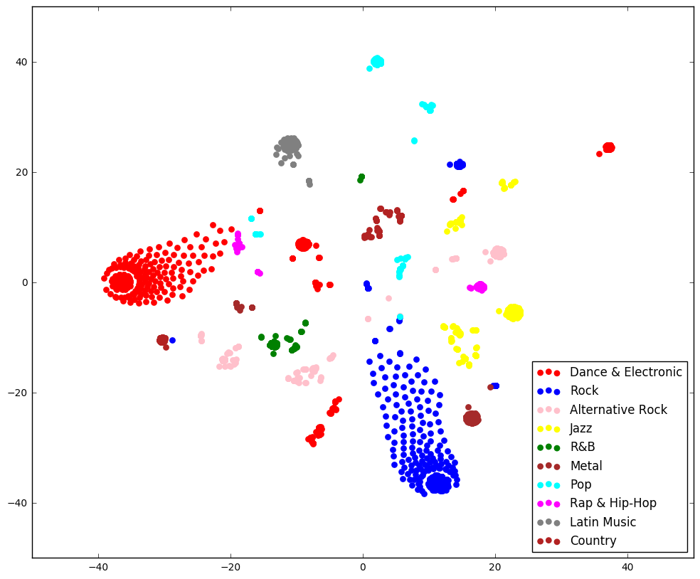
The matrix of album genre annotations of the training and validation sets is factorized using the approach described in Section 4.1, with a value of $d=50$ dimensions. From the set of album factors, those annotated with a single label from the top level of the taxonomy are plotted in Figure 1 using t-SNE dimensionality reduction [21]. It can be seen how the different albums are properly clustered in the factor space according to their genre.

6.1 Audio Classification

We explore three network design parameters: convolution filter size, number of filters per convolutional layer, and target layer. For the filter size we compare three approaches: square 3x3 filters as in [5], a filter of 4x96 that convolves only in time [45], and a musically motivated filter of 4x70, which is able to slightly convolve in the frequency domain [34]. To study the width of the convolutional layers we try with two different settings: high with 256, 512, 1024, and 1024 in each layer respectively, and low with 64, 128, 128, 64 filters. Max-pooling is applied after each convolutional layer. Finally, we use the two different network targets defined in Section 4, logistic and cosine. We empirically observed that dropout regularization only helps in the high plus cosine configurations. Therefore we applied dropout with a factor of 0.5 to these configurations, and no dropout to the others.

Apart from these configurations, a baseline approach is added. This approach consists in a traditional audio-based approach for genre classification based on the audio descriptors present in the MSD [1]. More specifically, for each song we aggregate four different statistics of the 12 timbre coefficient matrices: mean, max, variance, and $l2$-norm. The obtained 48 dimensional feature vectors are fed into a feed forward network as the one described in Section 5.4 with logistic output. This approach is denoted as timbre-mlp.

The results show that CNNs applied over audio spectrograms clearly outperform traditional approaches based on handcrafted features. We observe that the timbre-mlp approach achieves 0.792 of AUC, contrasting with the 0.888 from the best CNN approach. We note that the logistic configuration obtains better results when using a lower number of filters per convolution (low). Configurations with fewer filters have less parameters to optimize, and their training processes are faster. On the other hand, in cosine configurations we observe that the use of a higher number of filters tends to achieve better performance. It seems that the fine-grained regression of the factors benefits from wider convolutions. Moreover, we observe that 3x3 square filter settings have lower performance, need more time to train, and have a higher number of parameters to optimize. By contrast, networks using time convolutions only (4x96) have a lower number of parameters, are faster to train, and achieve comparable performance. Furthermore, networks that slightly convolve across the frequency bins (4x70) achieve better results with only a slightly higher number of parameters and training time. Finally, we observe that the cosine regression approach achieves better AUC scores in most configurations, and also their results are more diverse in terms of catalog coverage.

6.2 Text Classification

For text classification, we obtain two feature vectors as described in Section 5.2: one built from the texts VSM, and another built from the semantically enriched texts VSM+Sem. Both feature vectors are trained in the multi-label genre classification task using the two output configurations logistic and cosine.

Results show that the semantic enrichment of texts clearly yields better results in terms of AUC and diversity. Furthermore, we observe that the cosine configuration slightly outperforms logistic in terms of AUC, and greatly in terms of catalog coverage. The text-based results are overall slightly superior to the audio-based ones.

We also studied the information gain of words in the different genres. We observed that genre labels present in the texts have important information gain values. However, it is remarkable that band is a very informative word for Rock, song for Pop, and dope, rhymes, and beats are discriminative features for Rap albums. Place names have also important weights, as Jamaica for Reggae, Nashvile for Country, or Chicago for Blues.

6.3 Image Classification

Figure 2: Particular of the t-SNE of randomly selected image vectors from five of the most frequent genres.

Results show that genre classification from images has lower performance in terms of AUC and catalog coverage compared to the other modalities. Due to the use of an already pre-trained network with a logistic output (ImageNet [35]) as initialization of the network, it is not straightforward to apply the cosine configuration. Therefore, we only report results for the logistic configuration.

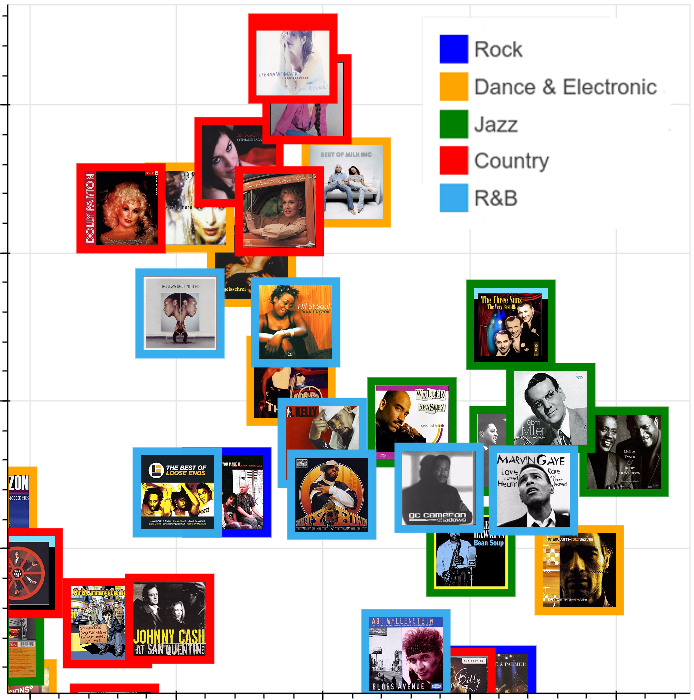
In Figure 2 a set of cover images of five of the most frequent genres in the dataset is shown using t-SNE over the obtained image feature vectors. In the left top corner the ResNet recognizes women faces on the foreground, which seems to be common in Country albums (red). The jazz albums (green) on the right are all clustered together probably thanks to the uniform type of clothing worn by the people of their covers. Therefore, the visual style of the cover seems to be informative when recognizing the album genre. For instance, many classical music albums include an instrument in the cover, and Dance & Electronics covers are often abstract images with bright colors, rarely including human faces.

6.4 Multimodal Classification

From the best performing approaches in terms of AUC of each modality (i.e., Audio / cosine / high-4x70, Text / cosine / VSM+Sem and Image / logistic / ResNet), a feature vector is obtained as described in Section 5.4. Then, these three feature vectors are aggregated in all possible combinations, and genre labels are predicted using the MLP network described in Section 5.4. Both output configurations logistic and cosine are used in the learning phase, and dropout of 0.7 is applied in the cosine configuration.

Results suggest that the combination of modalities outperforms single modality approaches. As image features are learned using a logistic configuration, they seem to improve multimodal approaches with logistic configuration only. Multimodal approaches that include text features tend to improve the results. Nevertheless, the best approaches are those that exploit the three modalities of MuMu. Cosine approaches have similar AUC than logistic approaches but a much better catalog coverage, thanks to the spatial properties of the factor space.

7 Conclusions

An approach for multi-label music genre classification using deep learning architectures has been proposed. The approach was applied to audio, text, image data, and their combination. For its assessment, MuMu, a new multimodal music dataset with over 31k albums and 135k songs has been gathered. We showed how representation learning approaches for audio classification outperform traditional handcrafted feature based approaches. Moreover, we compared the effect of different design parameters of CNNs in audio classification. Text-based approaches seem to outperform other modalities, and benefit from the semantic enrichment of texts via entity linking. While the image-based classification yielded the lowest performance, it helped to improve the results when combined with other modalities. Multimodal approaches appear to outperform single modality approaches, and the aggregation of the three modalities achieved the best results. Furtheremore, the dimensionality reduction of target labels led to better results, not only in terms of accuracy, but also in terms of catalog coverage.

This paper is an initial attempt to study the multi-label classification problem of music genres from different perspectives and using different data modalities. In addition, the release of the MuMu dataset opens up a number of unexplored research possibilities. In the near future we aim to modify the ResNet to be able to learn latent factors from images as we did in other modalities and apply the same multimodal approach to other MIR tasks.

8 Acknowledgments

This work was partially funded by the Spanish Ministry of Economy and Competitiveness under the Maria de Maeztu Units of Excellence Programme (MDM-2015-0502). The Tesla K40 used for this research was donated by the NVIDIA Corporation.

References

- [1] Thierry Bertin-Mahieux, Daniel P.W. Ellis, Brian Whitman, and Paul Lamere. The million song dataset. In ISMIR, 2011.
- [2] Dmitry Bogdanov, Alastair Porter, Perfecto Herrera, and Xavier Serra. Cross-collection evaluation for music classification tasks. In ISMIR, 2016.
- [3] Michael A Casey, Remco Veltkamp, Masataka Goto, Marc Leman, Christophe Rhodes, and Malcolm Slaney. Content-based music information retrieval: Current directions and future challenges. Proceedings of the IEEE, 96(4):668–696, 2008.
- [4] Kahyun Choi, Jin Ha Lee, and J Stephen Downie. What is this song about anyway?: Automatic classification of subject using user interpretations and lyrics. In Proceedings of the 14th ACM/IEEE-CS Joint Conference on Digital Libraries, pages 453–454. IEEE Press, 2014.
- [5] Keunwoo Choi, George Fazekas, and Mark Sandler. Automatic tagging using deep convolutional neural networks. ISMIR, 2016.
- [6] Keunwoo Choi, George Fazekas, Mark Sandler, and Kyunghyun Cho. Convolutional recurrent neural networks for music classification. arXiv preprint arXiv:1609.04243, 2016.
- [7] François Chollet. Information-theoretical label embeddings for large-scale image classification. CoRR, pages 1–10, 2016.
- [8] Sander Dieleman, Philémon Brakel, and Benjamin Schrauwen. Audio-based music classification with a pretrained convolutional network. In ISMIR, 2011.
- [9] Sander Dieleman and Benjamin Schrauwen. End-to-end learning for music audio. In Acoustics, Speech and Signal Processing (ICASSP), 2014 IEEE International Conference on, pages 6964–6968. IEEE, 2014.
- [10] Matthias Dorfer, Andreas Arzt, and Gerhard Widmer. Towards score following in sheet music images. ISMIR, 2016.
- [11] Kaiming He, Xiangyu Zhang, Shaoqing Ren, and Jian Sun. Deep residual learning for image recognition. In Proceedings of the IEEE Conference on Computer Vision and Pattern Recognition, pages 770–778, 2016.
- [12] Andrew G Howard. Some improvements on deep convolutional neural network based image classification. arXiv preprint arXiv:1312.5402, 2013.
- [13] Xiao Hu, J Stephen Downie, Kris West, and Andreas F Ehmann. Mining music reviews: Promising preliminary results. In ISMIR, 2005.
- [14] Himanshu Jain, Yashoteja Prabhu, and Manik Varma. Extreme multi-label loss functions for recommendation, tagging, ranking & other missing label applications. In Proceedings of the 22nd ACM SIGKDD International Conference on Knowledge Discovery and Data Mining, pages 935–944. ACM, 2016.
- [15] Yoon Kim. Convolutional Neural Networks for Sentence Classification. Proceedings of the 2014 Conference on Empirical Methods in Natural Language Processing (EMNLP 2014), pages 1746–1751, 2014.
- [16] Cyril Laurier, Jens Grivolla, and Perfecto Herrera. Multimodal music mood classification using audio and lyrics. In Machine Learning and Applications, 2008. ICMLA’08. Seventh International Conference on, pages 688–693. IEEE, 2008.
- [17] Omer Levy and Yoav Goldberg. Neural word embedding as implicit matrix factorization. In Advances in neural information processing systems, pages 2177–2185, 2014.
- [18] Janis Libeks and Douglas Turnbull. You can judge an artist by an album cover: Using images for music annotation. IEEE MultiMedia, 18(4):30–37, 2011.
- [19] Tsung-Yi Lin, Michael Maire, Serge Belongie, James Hays, Pietro Perona, Deva Ramanan, Piotr Dollár, and C Lawrence Zitnick. Microsoft coco: Common objects in context. In European Conference on Computer Vision, pages 740–755. Springer, 2014.
- [20] Beth Logan et al. Mel frequency cepstral coefficients for music modeling. In ISMIR, 2000.
- [21] Laurens van der Maaten and Geoffrey Hinton. Visualizing data using t-sne. Journal of Machine Learning Research, 9(Nov):2579–2605, 2008.
- [22] Rudolf Mayer, Robert Neumayer, and Andreas Rauber. Rhyme and style features for musical genre classification by song lyrics. In ISMIR, 2008.
- [23] Julian McAuley, Christopher Targett, Qinfeng Shi, and Anton Van Den Hengel. Image-based recommendations on styles and substitutes. In Proceedings of the 38th International ACM SIGIR Conference on Research and Development in Information Retrieval, pages 43–52. ACM, 2015.
- [24] Brian Mcfee, Colin Raffel, Dawen Liang, Daniel P W Ellis, Matt Mcvicar, Eric Battenberg, and Oriol Nieto. librosa: Audio and Music Signal Analysis in Python. Proc. of the 14th Python in Science Conf., (Scipy):1–7, 2015.
- [25] Tomas Mikolov, Ilya Sutskever, Kai Chen, Greg S Corrado, and Jeff Dean. Distributed representations of words and phrases and their compositionality. In Advances in Neural Information Processing Systems 26, pages 3111–3119. 2013.
- [26] Andrea Moro, Alessandro Raganato, and Roberto Navigli. Entity Linking meets Word Sense Disambiguation: A Unified Approach. Transactions of the Association for Computational Linguistics, 2:231–244, 2014.
- [27] Robert Neumayer and Andreas Rauber. Integration of text and audio features for genre classification in music information retrieval. In European Conference on Information Retrieval, pages 724–727. Springer, 2007.
- [28] Jiquan Ngiam, Aditya Khosla, Mingyu Kim, Juhan Nam, Honglak Lee, and Andrew Y Ng. Multimodal deep learning. In Proceedings of the 28th international conference on machine learning (ICML-11), pages 689–696, 2011.
- [29] Sergio Oramas, Luis Espinosa-Anke, Aonghus Lawlor, et al. Exploring customer reviews for music genre classification and evolutionary studies. In ISMIR, 2016.
- [30] Sergio Oramas, Francisco Gómez, Emilia Gómez, and Joaquín Mora. Flabase: Towards the creation of a flamenco music knowledge base. In ISMIR, 2015.
- [31] Sergio Oramas, Oriol Nieto, Mohamed Sordo, and Xavier Serra. A Deep Multimodal Approach for Cold-start Music Recommendation. ArXiv e-prints, June 2017.
- [32] Sergio Oramas, Vito Claudio Ostuni, Tommaso Di Noia, Xavier Serra, and Eugenio Di Sciascio. Sound and music recommendation with knowledge graphs. ACM Transactions on Intelligent Systems and Technology (TIST), 8(2):21, 2016.
- [33] François Pachet and Daniel Cazaly. A taxonomy of musical genres. In Content-Based Multimedia Information Access-Volume 2, pages 1238–1245, 2000.
- [34] Jordi Pons, Thomas Lidy, and Xavier Serra. Experimenting with musically motivated convolutional neural networks. In Content-Based Multimedia Indexing (CBMI), 2016 14th International Workshop on, pages 1–6. IEEE, 2016.
- [35] Olga Russakovsky, Jia Deng, Hao Su, Jonathan Krause, Sanjeev Satheesh, Sean Ma, Zhiheng Huang, Andrej Karpathy, Aditya Khosla, Michael Bernstein, Alexander C. Berg, and Li Fei-Fei. ImageNet Large Scale Visual Recognition Challenge. International Journal of Computer Vision (IJCV), 115(3):211–252, 2015.
- [36] Chris Sanden and John Z. Zhang. Enhancing multi-label music genre classification through ensemble techniques. In Proceedings of the 34th International ACM SIGIR Conference on Research and Development in Information Retrieval, SIGIR ’11, pages 705–714, New York, NY, USA, 2011. ACM.
- [37] Alexander Schindler and Andreas Rauber. An audio-visual approach to music genre classification through affective color features. In European Conference on Information Retrieval, pages 61–67. Springer, 2015.
- [38] Christian Schörkhuber and Anssi Klapuri. Constant-Q transform toolbox for music processing. 7th Sound and Music Computing Conference, (JANUARY):3–64, 2010.
- [39] Klaus Seyerlehner, Markus Schedl, Tim Pohle, and Peter Knees. Using block-level features for genre classification, tag classification and music similarity estimation. Submission to Audio Music Similarity and Retrieval Task of MIREX, 2010, 2010.
- [40] Bob L Sturm. A survey of evaluation in music genre recognition. In International Workshop on Adaptive Multimedia Retrieval, pages 29–66. Springer, 2012.
- [41] Christian Szegedy, Wei Liu, Yangqing Jia, Pierre Sermanet, Scott Reed, Dragomir Anguelov, Dumitru Erhan, Vincent Vanhoucke, and Andrew Rabinovich. Going deeper with convolutions. In Proceedings of the IEEE Conference on Computer Vision and Pattern Recognition, pages 1–9, 2015.
- [42] Christian Szegedy, Vincent Vanhoucke, Sergey Ioffe, Jon Shlens, and Zbigniew Wojna. Rethinking the inception architecture for computer vision. In Proceedings of the IEEE Conference on Computer Vision and Pattern Recognition, pages 2818–2826, 2016.
- [43] Grigorios Tsoumakas and Ioannis Katakis. Multi-label classification: An overview. International Journal of Data Warehousing and Mining, 3(3), 2006.
- [44] George Tzanetakis and Perry Cook. Musical genre classification of audio signals. IEEE Transactions on speech and audio processing, 10(5):293–302, 2002.
- [45] Aaron van den Oord, Sander Dieleman, and Benjamin Schrauwen. Deep content-based music recommendation. NIPS’13 Proceedings of the 26th International Conference on Neural Information Processing Systems, pages 2643–2651, 2013.
- [46] Fei Wang, Xin Wang, Bo Shao, Tao Li, and Mitsunori Ogihara. Tag integrated multi-label music style classification with hypergraph. In ISMIR, 2009.
- [47] Justin Zobel and Alistair Moffat. Exploring the similarity space. ACM SIGIR Forum, 32(1):18–34, 1998.