Interleaved Group Convolutions for Deep Neural Networks

Abstract

In this paper, we present a simple and modularized neural network architecture, named interleaved group convolutional neural networks (IGCNets). The main point lies in a novel building block, a pair of two successive interleaved group convolutions: primary group convolution and secondary group convolution. The two group convolutions are complementary: (i) the convolution on each partition in primary group convolution is a spatial convolution, while on each partition in secondary group convolution, the convolution is a point-wise convolution; (ii) the channels in the same secondary partition come from different primary partitions. We discuss one representative advantage: Wider than a regular convolution with the number of parameters and the computation complexity preserved. We also show that regular convolutions, group convolution with summation fusion, and the Xception block are special cases of interleaved group convolutions. Empirical results over standard benchmarks, CIFAR-$10$, CIFAR-$100$, SVHN and ImageNet demonstrate that our networks are more efficient in using parameters and computation complexity with similar or higher accuracy.

1 Introduction

Architecture design in deep convolutional neural networks has been attracting increasing interests. The basic design purpose is efficient in terms of computation and parameter with high accuracy. Various design dimensions have been considered, ranging from small kernels [15, 35, 33, 4, 14], identity mappings [10] or general multi-branch structures [38, 42, 22, 34, 35, 33] for easing the training of very deep networks, and multi-branch structures for increasing the width [34, 4, 14].

Our interest is to reduce the redundancy of convolutional kernels. The redundancy comes from two extents: the spatial extent and the channel extent. In the spatial extent, small kernels are developed, such as $3\times 3$, $3\times 1$, $1\times 3$ [35, 29, 17, 26, 18]. In the channel extent, group convolutions [42, 40] and channel-wise convolutions or separable filters [28, 4, 14], have been studied. Our work belongs to the kernel design in the channel extent.

In this paper, we present a novel network architecture, which is a stack of interleaved group convolution (IGC) blocks. Each block contains two group convolutions: primary group convolution and secondary group convolution, which are conducted on primary and secondary partitions, respectively. The primary partitions are obtained by simply splitting input channels, e.g., $L$ partitions with each containing $M$ channels, and there are $M$ secondary partitions, each containing $L$ channels that lie in different primary partitions. The primary group convolution performs the spatial convolution over each primary partition separately, and the secondary group convolution performs a $1\times 1$ convolution (point-wise convolution) over each secondary partition, blending the channels across partitions outputted by primary group convolution. Figure 1 illustrates the interleaved group convolution block.

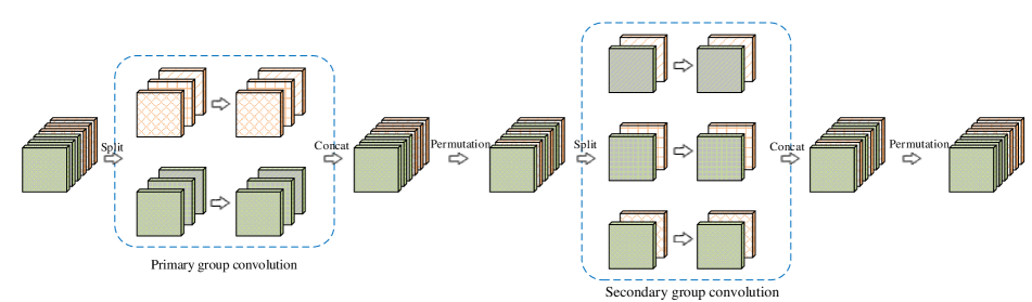
Figure 1: Illustrating the interleaved group convolution, with $L=2$ primary partitions and $M=3$ secondary partitions. The convolution for each primary partition in primary group convolution is spatial. The convolution for each secondary partition in secondary group convolution is point-wise ($1\times 1$). Details are given in Section 3.1.

It is known that a group convolution is equivalent to a regular convolution with sparse kernels: there is no connections across the channels in different partitions. Accordingly, an IGC block is equivalent to a regular convolution with the kernel composed from the product of two sparse kernels, resulting in a dense kernel. We show that under the same number of parameters/computation complexity, an IGC block (except the extreme case that the number of primary partitions, $L$, is $1$) is wider than a regular convolution with the spatial kernel size same to that of primary group convolution. Empirically, we also observe that a network built by stacking IGC blocks under the same computation complexity and the same number of parameters performs better than the network with regular convolutions.

We study the relations with existing related modules. (i) The regular convolution and group convolution with summation fusion [40, 42, 38], are both interleaved group convolutions, where the kernels are in special forms and are fixed in secondary group convolution. (ii) An IGC block in the extreme case where there is only one partition in the secondary group convolution, is very close to Xception [4].

Our main contributions are summarized as follows.

• We present a novel building block, interleaved group convolutions, which is efficient in parameter and computation.

• We show that the proposed building block is wider than a regular group convolution while keeping the network size and computational complexity, showing superior empirical performance.

• We discuss the connections to regular convolutions, the Xception block [4], and group convolution with summation fusion, and show that they are specific instances of interleaved group convolutions.

2 Related Works

Group convolutions and multi-branch. Group convolution is used in AlexNet [21] for distributing the model over two GPUs to handle the memory issue. The channel-wise convolutions used in the separable convolutions [28], is an extreme case of group convolutions, in which each partition contains only one channel.

The multi-branch architecture can be viewed as an extension of group convolutions by generalizing the convolution transformation on each partition, e.g., different number of convolution layers on different partitions, such as Inception [34], deeply-fused nets [38], a simple identity connection [10], and so on. Summation [40, 38], average [22], and convolution operations [34, 4] following concatenation are often adopted to blend the outputs. Our approach further improves parameter efficiency and adopts primary and secondary group convolutions, where secondary group convolution acts as a role of blending the channels outputted by primary group convolution.

Sparse convolutional kernels. Sparse convolution kernels have already been embedded into convolutional neural networks: the convolution filters usually have limited spatial extent. Low-rank filters [15, 17, 26] learn small basis filters, further sparsifying the connections. Channel-wise random sparse connection [2] sparsifies the filters in the channel extent that every output channel is connected to a small subset of input channels. There are some works introducing regularizations, such as structured sparsity regularizer [24, 39], $\ell_{1}$ or $\ell_{2}$ regularization [7, 8] on the kernel weights.

Our approach also sparsifies kernels in the channel extent, and differently, we use structured sparse connections in primary group convolution: both input and output convolutional channels are split to disjoint partitions and each output partition is connected to a single input partition and vice versa. In addition, we use secondary group convolution, another structured sparse filters, so that there is a path connecting each channel outputted by secondary group convolution to each channel fed into primary group convolution. Xception [4], which is shown to be more efficient than Inception [16], is close to our approach, and we show that it is a special case of our IGC block.

Decomposition. Tensor decomposition over each layer’s kernel (tensor) is widely-used to reduce redundancy of neural networks and compress/accelerate them. Tensor decomposition usually finds a low-rank tensor to approximate the tensor through decomposition along the spatial dimension [6, 17], or the input and output channel dimensions [6, 19, 17]. Rather than compressing previously-trained networks by approximating a convolution kernel using the product of two sparse kernels corresponding to our primary and secondary group convolutions, we train our network from scratch and show that our network can improve parameter efficiency and classification accuracy.

3 Our Network

3.1 Interleaved Group Convolutions

Definition. Our building block is based on group convolution, which is a method of dividing the input channels into several partitions and performing a regular convolution over each partition separately. A group convolution can be viewed as a regular convolution with a sparse block-diagonal convolution kernel, where each block corresponds to a partition of channels and there are no connections across the partitions.

Interleaved group convolutions consist of two group convolutions, primary group convolution and secondary group convolution. An example is shown in Figure 1. We use primary group convolutions to handle spatial correlation, and adopt spatial convolution kernels, e.g., $3\times 3$, widely-used in state-of-the-art networks [10, 29]. The convolutions are performed over each partition of channels separately. We use secondary group convolution to blend the channels across partitions outputted by primary group convolution and simply adopt $1\times 1$ convolution kernels.

Primary group convolutions. Let $L$ be the number of partitions, called primary partitions, in primary group convolution. We choose that each partition contains the same number ($M$) of channels. We simplify the discussion and present the group convolution over a single spatial position, and the formulation is easily obtained for all spatial positions. The primary group convolution is given as follows,

$$\begin{bmatrix}\mathbf{y}_{1}\\[3.00003pt] \mathbf{y}_{2}\\[3.00003pt] \vdots\\[3.00003pt] \mathbf{y}_{L}\end{bmatrix}=\begin{bmatrix}\mathbf{W}_{11}^{p}&\boldsymbol{0}&\boldsymbol{0}&\boldsymbol{0}\\[3.00003pt] \boldsymbol{0}&\mathbf{W}_{22}^{p}&\boldsymbol{0}&\boldsymbol{0}\\[3.00003pt] \vdots&\vdots&\ddots&\vdots\\[3.00003pt] \boldsymbol{0}&\boldsymbol{0}&\boldsymbol{0}&\mathbf{W}_{LL}^{p}\end{bmatrix}\begin{bmatrix}\mathbf{z}_{1}\\[3.00003pt] \mathbf{z}_{2}\\[3.00003pt] \vdots\\[3.00003pt] \mathbf{z}_{L}\end{bmatrix}.$$ (1)

Here $\mathbf{z}_{l}$ is a $(MS)$-dimensional vector, with $S$ being the kernel size, e.g., $9$ for $3\times 3$ kernels, and it is formed from the $S$ (e.g., $3\times 3$) responses around this spatial position for all the channels in this partition. $\mathbf{W}_{ll}^{p}$ corresponds to the convolutional kernel in the $l$th partition, and is a matrix of size $M\times(MS)$. Let $\mathbf{x}=[\mathbf{z}_{1}^{\top}~{}\mathbf{z}_{2}^{\top}~{}\dots~{}\mathbf{z}_{L}^{\top}]^{\top}$ represent the input of primary group convolution.

Secondary group convolutions. Our approach permutes the channels outputted by primary group convolution, $\{\mathbf{y}_{1},\mathbf{y}_{2},\dots,\mathbf{y}_{L}\}$, into $M$ secondary partitions with each partition consisting of $L$ channels, such that the channels in the same secondary partition come from different primary partitions. We adopt a simple scheme to form the secondary partitions: the $m$th secondary partition is composed of the $m$th output channel from each primary partition,

$$\bar{\mathbf{y}}_{m}=[y_{1m}~{}y_{2m}~{}\dots~{}y_{Lm}]^{\top}=\mathbf{P}_{m}^{\top}\mathbf{y},~{}\bar{\mathbf{y}}=\mathbf{P}^{\top}\mathbf{y}.$$ (2)

Here, $\bar{\mathbf{y}}_{m}$ corresponds to the $m$th secondary partition, $y_{lm}$ is the $m$th element of $\mathbf{y}_{l}$, $\bar{\mathbf{y}}=[\bar{\mathbf{y}}_{1}^{\top}~{}\bar{\mathbf{y}}_{2}^{\top}~{}\dots~{}\bar{\mathbf{y}}_{M}^{\top}]^{\top}$. $\mathbf{y}=[\mathbf{y}_{1}^{\top}~{}\mathbf{y}_{2}^{\top}~{}\dots~{}\mathbf{y}_{L}^{\top}]^{\top}$. $\mathbf{P}$ is the permutation matrix, and $\mathbf{P}=[\mathbf{P}_{1}~{}\mathbf{P}_{2}~{}\dots~{}\mathbf{P}_{M}]$.

The secondary group convolution is performed over the $M$ secondary partitions:

$$\bar{\mathbf{z}}_{m}=\mathbf{W}_{mm}^{d}\bar{\mathbf{y}}_{m},$$ (3)

where $\mathbf{W}_{mm}^{d}$ corresponds to the $1\times 1$ convolution kernel of the $m$th secondary partition, and is a matrix of size $L\times L$. The channels outputted by secondary group convolution are permuted back to the primary form as the input of the next interleaved group convolution block. The $L$ permuted-back partitions are given as follows, $\{\mathbf{x}_{1}^{\prime},\mathbf{x}_{2}^{\prime},\dots,\mathbf{x}_{L}^{\prime}\}$, and

$$\mathbf{x}_{l}^{\prime}=[\bar{z}_{1l}~{}\bar{z}_{2l}~{}\dots~{}\bar{z}_{Ml}]^{\top},~{}\mathbf{x}^{\prime}=\mathbf{P}\bar{\mathbf{z}},$$ (4)

where $\bar{\mathbf{z}}=[\bar{\mathbf{z}}_{1}^{\top}~{}\bar{\mathbf{z}}_{2}^{\top}~{}\dots~{}\bar{\mathbf{z}}_{M}^{\top}]^{\top}$.

In summary, an interleaved group convolution block is formulated as

$$\mathbf{x}^{\prime}=\mathbf{P}\mathbf{W}^{d}\mathbf{P}^{\top}\mathbf{W}^{p}\mathbf{x},$$ (5)

where $\mathbf{W}^{p}$ and $\mathbf{W}^{d}$ are block-diagonal matrices: $\mathbf{W}^{p}=\operatorname{diag}(\mathbf{W}_{11}^{p},\mathbf{W}_{22}^{p},\dots,\mathbf{W}_{LL}^{p})$ and $\mathbf{W}^{d}=\operatorname{diag}(\mathbf{W}_{11}^{d},\mathbf{W}_{22}^{d},\dots,\mathbf{W}_{MM}^{d})$.

Let $\mathbf{W}=\mathbf{P}\mathbf{W}^{d}\mathbf{P}^{\top}\mathbf{W}^{p}$ be the composite convolution kernel, then we have

$$\mathbf{x}^{\prime}=\mathbf{W}\mathbf{x},$$ (6)

which implies that an IGC block is equivalent to a regular convolution with the convolution kernel being the product of two sparse kernels.

3.2 Analysis

Wider than regular convolutions. Recall that the kernel size in the primary group convolution is $S$ and the kernel size in the secondary group convolution is $1$ ($=1\times 1$). Considering a single spatial position, the number of the parameters (equivalent to the computation complexity if the feature map size is fixed) in an IGC block is

$$T_{igc} =(L\cdot M\cdot M\cdot S+M\cdot L\cdot L)$$

$$=G^{2}\cdot(S/L+1/M),$$ (7)

where $G=ML$ is the width (the number of channels) of an IGC block.

Table 1: The widths of our interleaved group convolution block for various numbers of primary partitions $L$ and secondary partitions $M$ under the roughly-equal number of parameters: (i) $\approx~{}4672$ and (ii) $\approx~{}17536$. The kernel size $S$ of primary group convolution is $9=3\times 3$. The width $LM$ is the greatest when $L\approx 9M$: (i) $28\approx 3\times 9$ and (ii) $41\approx 5\times 9$.

	(i): #params $\approx~{}4672$									(ii): #params $\approx~{}17536$
$L$	$1$	$2$	$3$	$5$	$6$	$12$	$\bf{28}$	$40$	$64$	$1$	$2$	$4$	$12$	$14$	$23$	$28$	$\bf{41}$	$64$	$85$	$128$
$M$	$23$	$16$	$13$	$10$	$9$	$6$	$\bf{3}$	$2$	$1$	$44$	$31$	$22$	$12$	$11$	$8$	$7$	$\bf{5}$	$3$	$2$	$1$
#params	$4784$	$4672$	$4680$	$4750$	$4698$	$4752$	$\bf{4620}$	$4640$	$4672$	$17468$	$17422$	$17776$	$17280$	$17402$	$17480$	$17836$	$\bf{17630}$	$17472$	$17510$	$17536$
Width	$23$	$32$	$39$	$50$	$54$	$72$	$\bf{84}$	$80$	$64$	$44$	$63$	$88$	$144$	$154$	$184$	$196$	$\bf{205}$	$192$	$170$	$128$

For a regular convolution with the same kernel size $S$ and the input and output width being $C$, the number of parameters is

$$T_{rc}=C\cdot C\cdot S.$$ (8)

Given the same number of parameters, $T_{igc}=T_{rc}=T$, we have $C^{2}=\frac{1}{S}T$, and $G^{2}=\frac{1}{S/L+1/M}T$. It is easy to show that

$$G>C,~{}\textrm{when~{}}\frac{L}{L-1}<MS.$$ (9)

Considering the typical case $S=3\times 3$, we have $G>C$ when $L>1$. In other words, an IGC block is wider than a regular convolution, except the extreme case that there is only one partition in primary group convolution ($L=1$).

When is the widest? We discuss how the primary and secondary partition numbers $L$ and $M$ affect the width. Considering Equation 7, we have,

$$T_{igc}= ~{}L\cdot M\cdot M\cdot S+M\cdot L\cdot L$$ (10)

$$= ~{}LM(MS+L)$$ (11)

$$\geqslant ~{}LM\cdot 2\sqrt{LMS}$$ (12)

$$= ~{}2\sqrt{S}(LM)^{\frac{3}{2}}$$ (13)

$$= ~{}2\sqrt{S}G^{\frac{3}{2}},$$ (14)

where the equality in the third line holds when $L=MS$. It implies that (i) given the number of parameters, the width $G$ is upper-bounded,

$$G\leqslant\left(\frac{T_{igc}}{2\sqrt{S}}\right)^{\frac{2}{3}}.$$ (15)

and (ii) when $L=MS$, the width is the greatest.

Table 1 presents two examples. We can see that when $L\approx 9M$ ($S=9$), the width is the greatest: $3\times 9\approx 28$ for #params $\approx 4672$ and $5\times 9\approx 41$ for #params $\approx 17536$.

Wider leads to better performance? We have shown that an IGC block is equivalent to a single regular convolution, with the convolution kernel composed from two sparse kernels: $\mathbf{W}=\mathbf{P}\mathbf{W}^{d}\mathbf{P}^{\top}\mathbf{W}^{p}$. Fixing the parameter number means the following constraint,

$$\|\mathbf{W}^{p}\|_{0}+\|\mathbf{W}^{d}\|_{0}=T,$$ (16)

where $\|\cdot\|_{0}$ is an entry-wise $\ell_{0}$ norm of a matrix. This equation means that when the IGC is wider (or the dimension of the input $\mathbf{x}$ is higher), $\mathbf{W}^{p}$ and $\mathbf{W}^{d}$ are larger but more sparse. In other words, the composite convolution kernel $\mathbf{W}$ is more constrained as it becomes larger. Consequently, the increased width is probably not fully explored and the performance might not be improved, because of the constraint in the composite convolution kernel $\mathbf{W}$. Our empirical results shown in Figure 3 verify this point and suggest that an IGC block near the greatest width, e.g., $M=2$ in the two example cases in Figure 3, achieves the best performance.

4 Discussions and Connections

We show that regular convolutions, summation fusion preceded by group convolution as studied in ResNeXt [40] and the Xception block [4] are special IGC blocks, and discuss several possible extensions.

Connection to regular convolutions. A regular convolution over a single spatial position can be written as $\mathbf{x}^{\prime}=\mathbf{W}\mathbf{x}$, where $\mathbf{x}$ is the input, $\mathbf{W}$ is the weight matrix corresponding to the convolution kernel, and $\mathbf{x}^{\prime}$ is the output. We show the equivalent IGC form by taking $L=4$ as an example, which is illustrated in Figure 2. The general equivalence for other $L$ can be similarly derived.

Its IGC form is given as follows,

$$\bar{\mathbf{x}}^{\prime}= \mathbf{P}\mathbf{W}^{d}\mathbf{P}^{\top}\mathbf{W}^{p}\bar{\mathbf{x}}.$$ (17)

Here, $\bar{\mathbf{x}}=[\mathbf{x}^{\top}~{}\mathbf{x}^{\top}]^{\top}$, and $\bar{\mathbf{x}}^{\prime}=[\mathbf{x}^{\prime\top}~{}\mathbf{x}^{\prime\top}]^{\top}$. $\mathbf{W}^{p}$ is a block-diagonal matrix,

$$\mathbf{W}^{p}=\operatorname{diag}(\mathbf{W}_{11},\mathbf{W}_{12},\mathbf{W}_{21},\mathbf{W}_{22}).$$ (18)

$\mathbf{W}_{ij}$ is a block of $\mathbf{W}$ which is in the form of $2\times 2$ blocks,

$$\mathbf{W}=\begin{bmatrix}\mathbf{W}_{11}&\mathbf{W}_{12}\\[3.00003pt] \mathbf{W}_{21}&\mathbf{W}_{22}\end{bmatrix}.$$ (19)

$\mathbf{W}^{d}$ is a diagonal block matrix with $M$ ($=$ half of the dimension of $\mathbf{x}$) blocks of size $L\times L$, where $L=4$. All block matrices in $\mathbf{W}^{d}$ are the same:

$$\mathbf{W}_{11}^{d}=\mathbf{W}_{22}^{d}=\dots=\mathbf{W}_{MM}^{d}=\begin{bmatrix}1&1&0&0\\[3.00003pt] 0&0&1&1\\[3.00003pt] 1&1&0&0\\[3.00003pt] 0&0&1&1\end{bmatrix}.$$ (20)

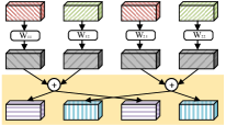
Figure 2: (a) Regular convolution. (b) Four-branch representation of the regular convolution. The shaded part in (b), we call cross-summation, is equivalent to a three-step transformation: permutation, secondary group convolution, and permutation back.

Connection to summation fusion. The summation fusion block [38] (like used in ResNeXt [40]), is composed of a group of branches, e.g., $L$ convolutions (as defined in Equation 1) followed by a summation operation, which is written as follows,

$$\mathbf{x}^{\prime}=\sum\nolimits_{i=1}^{L}\mathbf{y}_{i},$$ (21)

where $\mathbf{x}^{\prime}$ is the input of the next group convolution in which the inputs of all the branches are the same. Unlike the shaded part in Figure 2 for regular convolution, summation fusion receives all the four inputs and sum them together as the four outputs, which are the same.

In the form of interleaved group convolutions, the secondary group convolution is simple and the kernel parameters in each convolution are all $1$, i.e., the matrix $\mathbf{W}_{mm}^{d}$ in Equation 3 is an all-one matrix. For example, in the case that there are $4$ primary partitions,

$$\mathbf{W}_{11}^{d}=\mathbf{W}_{22}^{d}=\dots=\mathbf{W}_{MM}^{d}=\begin{bmatrix}1&1&1&1\\[3.00003pt] 1&1&1&1\\[3.00003pt] 1&1&1&1\\[3.00003pt] 1&1&1&1\end{bmatrix}.$$ (22)

Xception is an extreme case. We discuss two extreme cases: $L=1$ and $M=1$. In the case where $L=1$, the primary group convolution becomes a regular convolution, and the secondary group convolution behaves like assigning each channel with a different weight.

In the case where $M=1$, the primary group convolution becomes an extreme group convolution: a channel-wise group convolution, and the secondary group convolution becomes a $1\times 1$ convolution. This extreme case is close to Xception (standing for Extreme Inception) [4] that consists of a channel-wise spatial convolution preceded by a $1\times 1$ convolution. It is pointed in [4] that performing the $1\times 1$ convolution before or after the channel-wise spatial convolution does not make difference. Section 1 shows that the two extreme cases do not lead to the greater width except the trivial case that $L=9$ and $M=1$ ($L=9M$). Our empirical results shown in Figure 3 also indicate that $L=1$ performs poorly and $M=1$ performs well but not the best.

Extensions and variants. First, the convolution kernels in primary and secondary group convolutions are changeable: primary group convolution uses $1\times 1$ convolution kernels and secondary group convolution uses spatial (e.g., $3\times 3$) convolution kernels. Our empirical results show that such a change does not make difference. Second, secondary group convolution can be replaced by a linear projection, or a $1\times 1$ convolution, which also blends the channels across partitions outputted by primary group convolution. This results in a network like discussed in [4, 14]. Secondary group convolutions can also adopt spatial convolutions. Both are not our choice because extra parameters and computation complexity are introduced.

Last, our approach appears to be complementary to existing methods. Other spatial convolutional kernels, such as $3\times 1$ and $1\times 3$, can also be used in our primary group convolutions: decompose a $3\times 3$ kernel into two successive kernels, $3\times 1$ and $1\times 3$. The number of output channels of primary group convolution can also be decreased, which is like a bottleneck design. These potentially further improve the parameter efficiency.

Table 2: The architectures of networks with regular convolutions (RegConv-$Wc$ with $c$ being the channel number (width) at the first stage), with summation fusions (SumFusion), and with interleaved group convolutions (IGC-$L4M8$, IGC-$L24M2$, IGC-$L32M26$). $B$ is the number of blocks at each stage. $4\times(3\times 3,8)$ means a group convolution with $4$ partitions, with the convolution kernel on each partition being $(3\times 3,8)$.

Output size	SumFusion	RegConv-$Wc$	IGC-$L4M8$	IGC-$L24M2$	IGC-$L32M26$
$32\times 32$	$(3\times 3,8)$	$(3\times 3,c)$	$(3\times 3,32)$	$(3\times 3,48)$	$(3\times 3,26\times 32)$
$32\times 32$	$\begin{bmatrix}4\times(3\times 3,8)\\[2.40002pt] \operatorname{Summation}\end{bmatrix}\times B$	$(3\times 3,c)\times B$	$\begin{bmatrix}4\times(3\times 3,8)\\[2.40002pt] 8\times(1\times 1,4)\end{bmatrix}\times B$	$\begin{bmatrix}24\times(3\times 3,2)\\[2.40002pt] 2\times(1\times 1,24)\end{bmatrix}\times B$	$\begin{bmatrix}32\times(3\times 3,26)\\[2.40002pt] 26\times(1\times 1,32)\end{bmatrix}\times 6$
$16\times 16$	$\begin{bmatrix}4\times(3\times 3,16)\\[2.40002pt] \operatorname{Summation}\end{bmatrix}\times B$	$(3\times 3,2c)\times B$	$\begin{bmatrix}4\times(3\times 3,16)\\[2.40002pt] 16\times(1\times 1,4)\end{bmatrix}\times B$	$\begin{bmatrix}24\times(3\times 3,4)\\[2.40002pt] 4\times(1\times 1,24)\end{bmatrix}\times B$	$\begin{bmatrix}32\times(3\times 3,52)\\[2.40002pt] 52\times(1\times 1,32)\end{bmatrix}\times 6$
$8\times 8$	$\begin{bmatrix}4\times(3\times 3,32)\\[2.40002pt] \operatorname{Summation}\end{bmatrix}\times B$	$(3\times 3,4c)\times B$	$\begin{bmatrix}4\times(3\times 3,32)\\[2.40002pt] 32\times(1\times 1,4)\end{bmatrix}\times B$	$\begin{bmatrix}24\times(3\times 3,8)\\[2.40002pt] 8\times(1\times 1,24)\end{bmatrix}\times B$	$\begin{bmatrix}32\times(3\times 3,104)\\[2.40002pt] 104\times(1\times 1,32)\end{bmatrix}\times 6$
$1\times 1$	average pool, fc, softmax
Depth	$3B+2$				20

Table 3: The number of parameters of networks used in our experiments and the computation complexity in terms of FLOPs (# of multiply-adds). The statistics of the summation fusion networks are nearly the same with RegConv-$W16$ and are not included. For IGC-$L24M2$, the numbers of parameters are the smallest, and the computation complexities are the lowest.

D	#Params ($\times$M)				FLOPs ($\times 10^{8}$)
	RegConv-$W16$	RegConv-$W18$	IGC-$L4M8$	IGC-$L24M2$	RegConv-$W16$	RegConv-$W18$	IGC-$L4M8$	IGC-$L24M2$
$8$	$0.075$	$0.095$	$0.078$	$\mathbf{0.047}$	$0.122$	$0.154$	$0.131$	$\mathbf{0.099}$
$20$	$0.27$	$0.34$	$0.27$	$\mathbf{0.15}$	$0.406$	$0.513$	$0.424$	$\mathbf{0.288}$
$38$	$0.56$	$0.71$	$0.57$	$\mathbf{0.31}$	$0.830$	$1.05$	$0.862$	$\mathbf{0.571}$
$62$	$0.95$	$1.20$	$0.96$	$\mathbf{0.52}$	$1.40$	$1.77$	$1.45$	$\mathbf{0.948}$
$98$	$1.53$	$1.93$	$1.56$	$\mathbf{0.83}$	$2.25$	$2.84$	$2.32$	$\mathbf{1.51}$

Table 4: Classification accuracy comparison on CIFAR-$10$ and CIFAR-$100$ of the convolutional networks with regular convolutions (RegConv-$W16$, RegConv-$W18$), with summation fusions (SumFusion), and with interleaved group convolutions (IGC-$L4M8$, IGC-$L24M2$). The architecture description and the parameter number statistics are given in Table 2 and in Table 3.

	SumFusion	RegConv-$W16$	RegConv-$W18$	IGC-$L4M8$	IGC-$L24M2$
D	CIFAR-$10$
$8$	$84.94\pm 0.40$	$89.46\pm 0.16$	$90.30\pm 0.25$	$89.89\pm 0.24$	$\mathbf{90.31\pm 0.39}$
$20$	$88.71\pm 0.46$	$92.24\pm 0.17$	$92.55\pm 0.14$	$92.54\pm 0.37$	$\mathbf{92.84\pm 0.26}$
$38$	$86.95\pm 0.77$	$90.77\pm 0.23$	$91.57\pm 0.09$	$92.05\pm 0.76$	$\mathbf{92.24\pm 0.62}$
$62$	$82.66\pm 0.75$	$88.22\pm 0.91$	$88.60\pm 0.49$	$89.23\pm 0.89$	$\mathbf{90.03\pm 0.85}$
D	CIFAR-$100$
$8$	$52.01\pm 0.77$	$62.83\pm 0.32$	$64.70\pm 0.27$	$64.18\pm 0.70$	$\mathbf{65.60\pm 0.59}$
$20$	$59.33\pm 0.86$	$67.90\pm 0.14$	$68.71\pm 0.32$	$69.45\pm 0.69$	$\mathbf{70.54\pm 0.61}$
$38$	$57.18\pm 1.21$	$64.04\pm 0.42$	$65.00\pm 0.57$	$67.33\pm 0.48$	$\mathbf{69.56\pm 0.76}$
$62$	$48.68\pm 3.84$	$56.88\pm 1.16$	$58.52\pm 2.31$	$63.06\pm 1.42$	$\mathbf{65.84\pm 0.75}$

5 Experiments

5.1 Datasets.

CIFAR. The CIFAR datasets [20], CIFAR-$10$ and CIFAR-$100$, are subsets of the $80$ million tiny images [37]. Both datasets contain $60000$ $32\times 32$ color images with $50000$ images for training and $10000$ images for test. The CIFAR-$10$ dataset has $10$ classes containing $6000$ images each. There are $5000$ training images and $1000$ testing images per class. The CIFAR-$100$ dataset has $100$ classes containing $600$ images each. There are $500$ training images and $100$ testing images per class. The standard data augmentation scheme we adopt is widely used for this dataset [10, 13, 23, 12, 22, 25, 27, 31, 32]: we first zero-pad the images with $4$ pixels on each side, and then randomly crop them to produce $32\times 32$ images, followed by horizontally mirroring half of the images. We normalize the images by using the channel means and standard deviations.

SVHN. The Street View House Numbers (SVHN) dataset is obtained from house numbers in Google Street View images. SVHN contains $73,257$ training images, $26,032$ test images, and $531,131$ images as additional training. Following [13, 23, 25], we select out $400$ samples per class from the training set and $200$ samples from the additional set, and use the remaining images as the training set without any data augmentation.

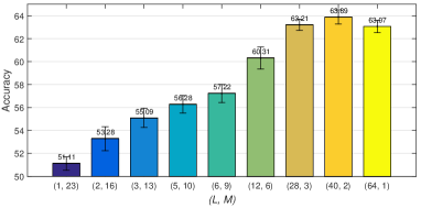
(a)    (b) 

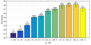
Figure 3: Illustrating the performances under different primary and secondary partition numbers $L$ and $M$ with same #params on CIFAR-$100$. We report the mean and the standard deviation over five runs. (a) corresponds to (i) in Table 1 and (b) corresponds to (ii) with more parameters.

5.2 Implementation Details

We adopt batch normalization (BN) [16] right after each IGC block and before nonlinear activation, i.e., IGC + BN + ReLU. We use the SGD algorithm with the Nesterov momentum, and train all networks from scratch. We initialize the weights similar to [9, 10, 12], and set the weight decay as $0.0001$ and the momentum as $0.9$.

On CIFAR-$10$ and CIFAR-$100$, we train all the models for $400$ epochs, with a total mini-batch size $64$ on two GPUs. The learning rate starts with $0.1$ and is reduced by a factor $10$ at the $200$, $300$, $350$ training epochs. On SVHN, we train $40$ epochs for all the models, with a total mini-batch size $64$ on two GPUs. The learning rate starts with $0.1$ and is reduced by a factor $10$ at the $20$, $30$, $35$ training epochs. Our implementation is based on MXNet [3].

Table 5: Illustrating that our approach benefits from identity mappings. Classification accuracy comparison on CIFAR-$10$ and CIFAR-$100$ between ResNets and our approach with identity mappings. Our network, IGC-$L24M2$+Ident. with fewer parameters and lower computation complexity (see Table 3), performs the best.

	RegConv-$W16$ + Ident.	RegConv-$W18$ + Ident.	IGC-$L4M8$ +Ident.	IGC-$L24M2$ +Ident.
Depth	CIFAR-$10$
$50$	$94.40\pm 0.45$	$94.67\pm 0.25$	$94.74\pm 0.54$	$\mathbf{94.88\pm 0.32}$
$74$	$94.66\pm 0.30$	$94.77\pm 0.59$	$94.79\pm 0.40$	$\mathbf{94.95\pm 0.23}$
$98$	$94.71\pm 0.44$	$94.95\pm 0.39$	$94.81\pm 0.30$	$\mathbf{95.15\pm 0.48}$
Depth	CIFAR-$100$
$50$	$72.98\pm 0.75$	$73.97\pm 0.49$	$74.00\pm 0.69$	$\mathbf{74.89\pm 0.67}$
$74$	$74.04\pm 0.62$	$74.55\pm 0.89$	$75.15\pm 0.49$	$\mathbf{75.41\pm 0.75}$
$98$	$74.49\pm 0.66$	$75.30\pm 0.88$	$75.58\pm 0.80$	$\mathbf{76.15\pm 0.50}$

Table 6: Imagenet classification results of a ResNet of depth $18$ and our approach. The network structure for ResNet can be found in [10]. Both ResNets and our networks contain four stages, and when down-sampling is performed, the channel number is doubled. For ResNets, $C$ is the channel number at the first stage. For our networks except IGC-$L100M2$+Ident., we double the channel number by doubling $M$ and keeping $L$ unchanged. For IGC-$L100M2$+Ident., we double the channel number by doubling $L$ and keeping $M$ unchanged.

	#Params	FLOPs	training error		testing error
	($\times$M)	($\times 10^{9}$)	top-1	top-5	top-1	top-5
ResNet ($C=64$)	$11.151$	$1.8$	$22.41$	$6.53$	$31.06$	$11.38$
ResNet ($C=69$)	$11.333$	$2.1$	$21.43$	$5.96$	$30.58$	$10.77$
IGC-$L4M32$+Ident.	$11.205$	$1.9$	$21.71$	$6.21$	$30.77$	$10.99$
IGC-$L16M16$+Ident.	$11.329$	$2.2$	${19.97}$	${5.44}$	${29.40}$	${10.32}$
IGC-$L100M2$+Ident.	$8.61$	$1.3$	$\mathbf{13.93}$	$\mathbf{2.75}$	$\mathbf{26.95}$	$\mathbf{8.92}$

Table 7: Classification error comparison with the state-of-the-arts. The best, second-best, and third-best accuracies are highlighted in red, green, and blue.

	Depth	#Params	CIFAR-$10$	CIFAR-$100$	SVHN
Network in Network [25]	-	-	$8.81$	$35.68$	$2.35$
All-CNN [31]	-	-	$7.25$	$33.71$	-
FitNet [27]	-	-	$8.39$	$35.04$	$2.42$
Deeply-Supervised Nets [23]	-	-	$8.22$	$34.57$	$1.92$
Swapout [30]	$20$	$1.1$M	$6.58$	$25.86$	-
	$32$	$7.4$M	$4.76$	$22.72$	-
Highway [32]	-	-	$7.72$	$32.39$	-
DFN [38]	$50$	$3.7$M	$6.40$	$27.61$	-
	$50$	$3.9$M	$6.24$	$27.52$	-
FractalNet [22]	$21$	$38.6$M	$5.22$	$23.30$	$2.01$
With dropout & droppath	$21$	$38.6$M	$4.60$	$23.73$	$1.87$
ResNet [10]	$110$	$1.7$M	$6.61$	-	-
ResNet [13]	$110$	$1.7$M	$6.41$	$27.76$	$1.80$
ResNet (pre-activation) [11]	$164$	$1.7$M	$5.46$	$24.33$	-
	$1001$	$10.2$M	$4.92$	$22.71$	-
ResNet with stochastic depth [13]	$110$	$1.7$M	$5.25$	$24.98$	$1.75$
	$1202$	$10.2$M	$4.91$	-	-
Wide ResNet [41]	$16$	$11.0$M	$4.27$	$20.43$	-
	$28$	$36.5$M	$4.00$	$19.25$	-
With dropout	$16$	$2.7$M	-	-	$1.64$
RiR [36]	$18$	$10.3$M	$5.01$	$22.90$	-
Multi-ResNet [1]	$200$	$10.2$M	$4.35$	$20.42$	-
	$26$	$72$M	$3.96$	$19.45$	-
DenseNet ($k=24$) [12]	$100$	$27.2$M	$3.74$	$19.25$	$1.59$
DenseNet-BC ($k=24$) [12]	$250$	$15.3$M	$3.62$	$\mathbf{17.60}$	$1.74$
DenseNet-BC ($k=40$) [12]	$190$	$25.6$M	$3.46$	$\mathbf{17.18}$	$-$
ResNeXt-29, $8\times 64$d [40]	$29$	$34.4$M	${3.65}$	${17.77}$	$-$
ResNeXt-29, $16\times 64$d [40]	$29$	$68.1$M	${3.58}$	$\mathbf{17.31}$	$-$
DFN-MR1 [42]	$56$	$1.7$M	${4.94}$	${24.46}$	$1.66$
DFN-MR2 [42]	$32$	$14.9$M	$3.94$	$19.25$	$\mathbf{1.51}$
DFN-MR3 [42]	$50$	$24.8$M	$3.57$	$19.00$	$\mathbf{1.55}$
IGC-$L16M32$	$20$	$17.7$M	$\mathbf{3.37}$	$19.31$	$1.63$
IGC-$L450M2$	$20$	$19.3$M	$\mathbf{3.25}$	${19.25}$	$-$
IGC-$L32M26$	$20$	$24.1$M	$\mathbf{3.31}$	${18.75}$	$\mathbf{1.56}$

5.3 Empirical Study

Comparison with regular convolution and summation fusion. We compare five networks: convolutional networks with regular convolutions (RegConv-$W16$, RegConv-$W18$), with summation fusions (SumFusion), and with interleaved group convolution blocks (IGC-$L4M8$, IGC-$L24M2$). Network architectures, parameter numbers and computation complexities are given in Table 2 and in Table 3.

The comparisons on CIFAR-$10$ and CIFAR-$100$ are given in Table 4. It can be seen that the overall performance of our networks, IGC-$L4M8$, are better than both RegConv-$W16$ containing slightly fewer parameters and RegConv-$W18$ containing more parameters, demonstrating that our IGC block is more powerful than regular convolutions. Another model, IGC-$L24M2$, containing much fewer parameters, performs better than both RegConv-$W16$ and RegConv-$W18$. The main reason lies in the advantage that our IGC blocks increase the width and the parameters are exploited more efficiently. For example, on CIFAR-$100$, when the depth is $38$, IGC-$L4M8$ and IGC-$L24M2$ achieve $67.33\%$, $69.56\%$ accuracy, about $2.3\%$, $4.5\%$ better than RegConv-$W18$. The summation fusion (SumFusion) performs worse because the summation fusion reduces the width and the parameters are not very efficiently used.

The effect of partition numbers. We have shown that how the numbers of primary and secondary partitions affect the width and one extreme case of our approach is Xception [4]. Now we empirically study how the performances are affected by the partition numbers and show that a typical setup, $M=2$, performs better than Xception [4].

To clearly show the effect, we use networks with $8$ layers: $6$ IGC blocks, the first convolution layer, and the last FC layer. There is no down-sampling stage: the map is always of size $32\times 32$. We change the partition numbers, $L$ and $M$, to guarantee the model size (the computation complexity) almost the same. We consider two cases for an IGC block: (i) the parameter number ($9LM^{2}+ML^{2}$) is approximately $4672$ and (ii) the parameter number is approximately $17536$ (see Table 1).

The results are presented in Figure 3. It can be observed that the accuracy increases when the number of primary partitions becomes larger (the number of secondary partitions becomes smaller) till it reaches some number and then decreases. In the two cases, the performance with $M=2$ secondary partitions is better than Xception. For example, in case (i), IGC with $L=40$ and $M=2$ gets $63.89\%$ accuracy, about $0.8\%$ better than IGC with $L=64$ and $M=1$, which gets $63.07\%$ accuracy. We believe that the performance in general is a concave function with respect to $M$ (or $L$) under roughly the same number of parameters, and the performance is not the best when $M=1$ (i.e., Xception [4]) or $L=1$.

Combination with identity mappings. We show that our IGCNet also benefits from identity mappings and achieves superior performance over ResNets [10]. We compare two networks with regular convolutions, RegConv-$W16$ and RegConv-$W18$, with IGC-$L4M8$ and IGC-$L24M2$. The residual branch consists of two regular convolution layers for ResNets [10] and two IGC blocks for our networks.

The results are shown in Table 5. One can see that our approaches, IGC-$L4M8$ + Ident. and IGC-$L24M2$+Ident., do not suffer from training difficulty because of identity mappings. IGC-$L4M8$+Ident. performs better (e.g., about $1\%$ accuracy improvement on CIFAR-$100$ with slightly more parameters, see Table 3) than RegConv-$W16$ + Ident., and performs similar (with smaller #parameters and computation complexity, see Table 3) to RegConv-$W18$+Ident.. In addition, IGC-$L24M2$+Ident., with fewer parameters and lower computation complexity (see Table 3), performs better than both RegConv-$W16$+Ident. and RegConv-$W18$+Ident., which again demonstrates that our IGC block can exploit the parameters efficiently.

ImageNet classification. We present the comparison to ResNets [10] for ImageNet classification. The ILSVRC $2012$ classification dataset [5] contains over $1.2$ million training images and $50,000$ validation images, and each image is labeled from $1000$ categories. We adopt the same data augmentation scheme for the training images as in [10, 11]. The models are trained for $95$ epochs with a total mini-batch size $256$ on $8$ GPUs. The learning rate starts with $0.1$ and is reduced by a factor $10$ at the $30$, $60$, $90$ epochs. A single $224\times 224$ center crop from an image is used to evaluate at test time. Our purpose is not to push the state-of-the-art results, but to demonstrate the powerfulness of our approach. So we use the comparison to ResNet-$18$ as an example.

The result is depicted in Table 6. (i) Our approach, IGC-$L4M32$+Ident., performs better than ResNet ($C=64$) that contains slightly fewer parameters. (ii) Our approach IGC-$L16M16$+Ident. performs better than ResNet ($C=69$) that has approximately the same number of parameters and computation complexity: our model gets about $1.5\%$ reduction for top-$1$ error and $1\%$ reduction for top-$5$ error. (iii) Our approach IGC-$L100M2$+Ident. gets the best result with a much smaller number of parameters and smaller computation complexity. We also notice that the training error of our approach is smaller than ResNets, suggesting that the gains are not from regularization but from richer representation.

5.4 Comparison with the State-of-the-Arts

We compare our approach with the state-of-the-art algorithms. The comparisons are reported in Table 7. We do not optimally tune the partition numbers for our network since the NVIDIA CuDNN library does not support group convolutions yet, making the group convolution operation slow in practical implementation.

Our networks contain $20$ layers: $18$ interleaved group convolution blocks, the first convolution layer and the last FC layer (see IGC-$L32M26$ in Table 3 as an example. We double the width by doubling $M$ when down-sampling the feature map at each stage). The best, second-best, and third-best accuracies are highlighted in red, green, and blue. It can be seen that our networks achieve competitive performance: the best accuracy on CIFAR-$10$, and the third-best accuracy on SVHN (close to the second-best accuracy). Our performance would be better if our network also adopts the bottleneck design as in DenseNet-BC [12] and ResNeXt [40] or adopts more primary partitions.

6 Conclusion

In this paper, we present a novel convolutional neural network architecture, which addresses the redundancy problem of convolutional filters in the channel domain. The main novelty lies in an interleaved group convolution block: channels in the same partition in the secondary group convolution come from different partitions used in the primary group convolution. Experimental results demonstrate that our network is efficient in parameter and computation.

Appendices

Table 8: Example configurations of GPCs for various numbers ($L$) of partitions and various numbers ($M$) of channels in each partition, under the roughly-equal number of parameters: (i) $\approx~{}4672$ and (ii) $\approx~{}17536$. The kernel size $S$ in group convolutions is $9=3\times 3$.

	(i) #params $\approx~{}4672$									(ii) #params $\approx~{}17536$
	GPC								IGC	GPC										IGC
$L$	$1$	$2$	$3$	$5$	$10$	$19$	$30$	$64$	$40$	$1$	$2$	$3$	$6$	$11$	$15$	$18$	$29$	$62$	$128$	$85$
$M$	$22$	$15$	$12$	$8$	$5$	$3$	$2$	$1$	$2$	$42$	$28$	$22$	$14$	$9$	$7$	$6$	$4$	$2$	$1$	$2$
#params	$4840$	$4950$	$5184$	$4480$	$4750$	$4788$	$4680$	$4672$	$4640$	$17640$	$17248$	$17424$	$17820$	$17640$	$17496$	$17632$	$17640$	$17608$	$17532$	$17510$
Width	$22$	$30$	$36$	$40$	$50$	$54$	$60$	$64$	$80$	$42$	$56$	$66$	$84$	$99$	$105$	$108$	$116$	$124$	$128$	$170$

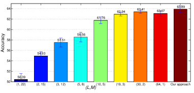
(a)    (b) 

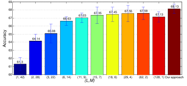
Figure 4: Illustrating the performances between our approach and the networks stacking GPC with various numbers $L$ and $M$ with same #params on CIFAR-$100$. We report the mean and the standard deviation over five runs. (a) corresponds to (i) in Table 8 and (b) corresponds to (ii) with more parameters.

Comparison with alternative structures. The proposed network is a stack of interleaved group convolution (IGC) blocks, where secondary group convolutions to blend the channels across partitions outputted by primary group convolutions.

In the main paper (Extensions and variants, Section 4), we discuss that a point-wise convolution, i.e., a $1\times 1$ convolution, as an alternative of secondary group convolutions, introduces extra parameters and computation complexity. Such an alternative is also mentioned or discussed in Xception [4] and deep roots [14]. We denote this alternative block as Group-and-Point-wise Convolution (GPC). The number of parameters for one GPC block is $L\cdot M\cdot M\cdot S+L\cdot M\cdot L\cdot M$, where $L$ is the number of partitions in group convolution, $M$ is the number of channels in each partition, and thus $LM$ is the number of total channels.

We replace IGC blocks in our networks using GPC blocks, with almost the same number of parameters. Table 8 presents the configurations: (i) #params $\approx 4672$ and (ii) #params $\approx 17536$ (See Table 1 in the main paper for the configurations of our IGC blocks). The results, together with our approach (with two secondary partitions) are presented in Figure 4 (More results about our networks are shown in Figure 3 in the main paper). We can see that our networks perform better and achieve around $0.5\%$ improvement in both cases.

More on the connection to regular convolutions. We rewrite Equation 17 as the following,

$$\bar{\mathbf{x}}^{\prime}= \mathbf{P}\mathbf{W}^{d}\mathbf{P}^{\top}\mathbf{W}^{p}\bar{\mathbf{x}}.$$ (23)

We discuss an extreme case: primary group convolution is a channel-wise convolution. Let

$$\bar{\mathbf{x}}=[\mathbf{x}^{\top}\mathbf{x}^{\top}~{}\dots~{}\mathbf{x}^{\top}]^{\top}.$$

be formed by concatenating $\mathbf{x}$ $C$ times. The primary group convolution is given as follows,

$$\mathbf{W}^{p}=\operatorname{diag}( \mathbf{w}_{11}^{\top},\mathbf{w}_{12}^{\top},\dots,\mathbf{w}_{1C}^{\top},$$ (24)

$$\mathbf{w}_{21}^{\top},\mathbf{w}_{22}^{\top},\dots,\mathbf{w}_{2C}^{\top},$$ (25)

$$~{}~{}~{}~{}~{}~{}~{}~{}~{}~{}~{}~{}~{}\dots,$$ (26)

$$\mathbf{w}_{C1}^{\top},\mathbf{w}_{C2}^{\top},\dots,\mathbf{w}_{CC}^{\top}),$$ (27)

where $\mathbf{w}_{ij}$ is a vector of $3\times 3$. The secondary group convolution is given as follows,

$$\mathbf{W}^{d}=\begin{bmatrix}\mathbf{1}^{\top}&\mathbf{0}^{\top}&\mathbf{0}^{\top}&\mathbf{0}^{\top}\\[3.00003pt] \mathbf{0}^{\top}&\mathbf{1}^{\top}&\mathbf{0}^{\top}&\mathbf{0}^{\top}\\[3.00003pt] \dots&\dots&\dots&\dots\\[3.00003pt] \mathbf{0}^{\top}&\mathbf{0}^{\top}&\dots&\mathbf{1}^{\top}\\[3.00003pt] \vdots&\vdots&\vdots&\vdots\\[3.00003pt] \mathbf{1}^{\top}&\mathbf{0}^{\top}&\mathbf{0}^{\top}&\mathbf{0}^{\top}\\[3.00003pt] \mathbf{0}^{\top}&\mathbf{1}^{\top}&\mathbf{0}^{\top}&\mathbf{0}^{\top}\\[3.00003pt] \dots&\dots&\dots&\dots\\[3.00003pt] \mathbf{0}^{\top}&\mathbf{0}^{\top}&\dots&\mathbf{1}^{\top}\\[3.00003pt] \end{bmatrix},$$ (28)

where $\mathbf{1}$ is a vector of $C$ ones, $\mathbf{0}$ is a vector of $C$ zeros. $\mathbf{W}^{d}$ consists of $C\times 1$ blocks, with each block being a matrix of $C\times C^{2}$. Thus, we have

$$\bar{\mathbf{x}}=[\mathbf{x}^{\prime\top}\mathbf{x}^{\prime\top}~{}\dots~{}\mathbf{x}^{\prime\top}]^{\top}.$$

References

- [1] M. Abdi and S. Nahavandi. Multi-residual networks. CoRR, abs/1609.05672, 2016.
- [2] S. Changpinyo, M. Sandler, and A. Zhmoginov. The power of sparsity in convolutional neural networks. CoRR, abs/1702.06257, 2017.
- [3] T. Chen, M. Li, Y. Li, M. Lin, N. Wang, M. Wang, T. Xiao, B. Xu, C. Zhang, and Z. Zhang. Mxnet: A flexible and efficient machine learning library for heterogeneous distributed systems. CoRR, abs/1512.01274, 2015.
- [4] F. Chollet. Xception: Deep learning with depthwise separable convolutions. CoRR, abs/1610.02357, 2016.
- [5] J. Deng, W. Dong, R. Socher, L. Li, K. Li, and F. Li. Imagenet: A large-scale hierarchical image database. In CVPR, pages 248–255, 2009.
- [6] E. L. Denton, W. Zaremba, J. Bruna, Y. LeCun, and R. Fergus. Exploiting linear structure within convolutional networks for efficient evaluation. In NIPS, pages 1269–1277, 2014.
- [7] S. Han, H. Mao, and W. J. Dally. Deep compression: Compressing deep neural network with pruning, trained quantization and huffman coding. CoRR, abs/1510.00149, 2015.
- [8] S. Han, J. Pool, J. Tran, and W. J. Dally. Learning both weights and connections for efficient neural network. In NIPS, pages 1135–1143, 2015.
- [9] K. He, X. Zhang, S. Ren, and J. Sun. Delving deep into rectifiers: Surpassing human-level performance on imagenet classification. In ICCV, pages 1026–1034, 2015.
- [10] K. He, X. Zhang, S. Ren, and J. Sun. Deep residual learning for image recognition. In CVPR, pages 770–778, 2016.
- [11] K. He, X. Zhang, S. Ren, and J. Sun. Identity mappings in deep residual networks. In ECCV, pages 630–645, 2016.
- [12] G. Huang, Z. Liu, and K. Q. Weinberger. Densely connected convolutional networks. CoRR, abs/1608.06993, 2016.
- [13] G. Huang, Y. Sun, Z. Liu, D. Sedra, and K. Q. Weinberger. Deep networks with stochastic depth. In ECCV, pages 646–661, 2016.
- [14] Y. Ioannou, D. P. Robertson, R. Cipolla, and A. Criminisi. Deep roots: Improving CNN efficiency with hierarchical filter groups. CoRR, abs/1605.06489, 2016.
- [15] Y. Ioannou, D. P. Robertson, J. Shotton, R. Cipolla, and A. Criminisi. Training cnns with low-rank filters for efficient image classification. CoRR, abs/1511.06744, 2015.
- [16] S. Ioffe and C. Szegedy. Batch normalization: Accelerating deep network training by reducing internal covariate shift. In ICML, pages 448–456, 2015.
- [17] M. Jaderberg, A. Vedaldi, and A. Zisserman. Speeding up convolutional neural networks with low rank expansions. In BMVC, 2014.
- [18] J. Jin, A. Dundar, and E. Culurciello. Flattened convolutional neural networks for feedforward acceleration. CoRR, abs/1412.5474, 2014.
- [19] Y. Kim, E. Park, S. Yoo, T. Choi, L. Yang, and D. Shin. Compression of deep convolutional neural networks for fast and low power mobile applications. CoRR, abs/1511.06530, 2015.
- [20] A. Krizhevsky. Learning multiple layers of features from tiny images. Technical report, 2009.
- [21] A. Krizhevsky, I. Sutskever, and G. E. Hinton. Imagenet classification with deep convolutional neural networks. In NIPS, pages 1106–1114, 2012.
- [22] G. Larsson, M. Maire, and G. Shakhnarovich. Fractalnet: Ultra-deep neural networks without residuals. CoRR, abs/1605.07648, 2016.
- [23] C. Lee, S. Xie, P. W. Gallagher, Z. Zhang, and Z. Tu. Deeply-supervised nets. In AISTATS, 2015.
- [24] H. Li, A. Kadav, I. Durdanovic, H. Samet, and H. P. Graf. Pruning filters for efficient convnets. CoRR, abs/1608.08710, 2016.
- [25] M. Lin, Q. Chen, and S. Yan. Network in network. CoRR, abs/1312.4400, 2013.
- [26] F. Mamalet and C. Garcia. Simplifying convnets for fast learning. In ICANN, pages 58–65, 2012.
- [27] A. Romero, N. Ballas, S. E. Kahou, A. Chassang, C. Gatta, and Y. Bengio. Fitnets: Hints for thin deep nets. CoRR, abs/1412.6550, 2014.
- [28] L. Sifre and S. Mallat. Rigid-motion scattering for texture classification. CoRR, abs/1403.1687, 2014.
- [29] K. Simonyan and A. Zisserman. Very deep convolutional networks for large-scale image recognition. CoRR, abs/1409.1556, 2014.
- [30] S. Singh, D. Hoiem, and D. A. Forsyth. Swapout: Learning an ensemble of deep architectures. In NIPS, pages 28–36, 2016.
- [31] J. T. Springenberg, A. Dosovitskiy, T. Brox, and M. A. Riedmiller. Striving for simplicity: The all convolutional net. CoRR, abs/1412.6806, 2014.
- [32] R. K. Srivastava, K. Greff, and J. Schmidhuber. Training very deep networks. In NIPS, pages 2377–2385, 2015.
- [33] C. Szegedy, S. Ioffe, V. Vanhoucke, and A. A. Alemi. Inception-v4, inception-resnet and the impact of residual connections on learning. In AAAI, pages 4278–4284, 2017.
- [34] C. Szegedy, W. Liu, Y. Jia, P. Sermanet, S. E. Reed, D. Anguelov, D. Erhan, V. Vanhoucke, and A. Rabinovich. Going deeper with convolutions. In CVPR, pages 1–9, 2015.
- [35] C. Szegedy, V. Vanhoucke, S. Ioffe, J. Shlens, and Z. Wojna. Rethinking the inception architecture for computer vision. In CVPR, pages 2818–2826, 2016.
- [36] S. Targ, D. Almeida, and K. Lyman. Resnet in resnet: Generalizing residual architectures. CoRR, abs/1603.08029, 2016.
- [37] A. Torralba, R. Fergus, and W. T. Freeman. 80 million tiny images: A large data set for nonparametric object and scene recognition. IEEE Trans. Pattern Anal. Mach. Intell., 30(11):1958–1970, 2008.
- [38] J. Wang, Z. Wei, T. Zhang, and W. Zeng. Deeply-fused nets. CoRR, abs/1605.07716, 2016.
- [39] W. Wen, C. Wu, Y. Wang, Y. Chen, and H. Li. Learning structured sparsity in deep neural networks. In NIPS, pages 2074–2082, 2016.
- [40] S. Xie, R. B. Girshick, P. Dollár, Z. Tu, and K. He. Aggregated residual transformations for deep neural networks. CoRR, abs/1611.05431, 2016.
- [41] S. Zagoruyko and N. Komodakis. Wide residual networks. CoRR, abs/1605.07146, 2016.
- [42] L. Zhao, J. Wang, X. Li, Z. Tu, and W. Zeng. On the connection of deep fusion to ensembling. CoRR, abs/1611.07718, 2016.