A Semiclassical “Divide-and-Conquer” Method for Spectroscopic Calculations of High Dimensional Molecular Systems

Abstract

A new semiclassical “divide-and-conquer” approach is presented with the aim to demonstrate that quantum dynamics simulations of high dimensional molecular systems are doable. The method is first tested by calculating the quantum vibrational power spectra of water, methane and benzene, three molecules of increasing dimensionality for which benchmark quantum results are available, and then applied to C₆₀, a system characterized by 174 vibrational degrees of freedom. Results show that the approach can accurately account for quantum anharmonicities, purely quantum features like overtones, and removal of degeneracy when the molecular symmetry is broken.

Quantum computational approaches to the spectroscopy of small or medium-size molecules are very popular. Among them we recall variational methods like vibrational configuration interaction (VCI)(Bowman et al., 2003; Samanta et al., 2016; Qu et al., 2015; Avila and Carrington Jr, 2011) and Multi Configuration Time Dependent Hartree (MCTDH),(Manthe, 2002; Meyer and Worth, 2003; Bowman et al., 2008) or perturbative ones, such as the second-order vibrational perturbation theory (VPT2).(Bludsky et al., 2000; Barone, 2005; Biczysko et al., 2012) Spectroscopy of high dimensional systems is more difficult to perform, since exact quantum simulations are unaffordable and even experimental spectra are often too crowded for an undisputed assignment. A new computationally-affordable strategy is needed, while spectra would certainly be much easier to read if they were decomposed into several partial ones.
For this purpose, a novel theoretical approach is here presented. It is based on a semiclassical (SC) “divide-and-conquer” strategy that leads to reliable calculations of higher dimensional systems than those ordinarily affordable with quantum methods. Full spectra are regained as a collection of partial ones, quantum effects are included, and a sound spectroscopic interpretation is obtained. This new method fills in the gap between a purely classical spectroscopic study, which is not satisfactory because it neglects key quantum features, and quantum approaches, which often require the set-up of a grid of points with a computational cost that exponentially scales with the dimensionality of the system.
In a semiclassical approach(Elran and Kay, 1999; Zhang and Pollak, 2004; Kay, 2006; Conte and Pollak, 2010; Bonella et al., 2010; Monteferrante et al., 2013; Conte and Pollak, 2012; Petersen and Pollak, 2015; Shalashilin and Child, 2001, 2004; Heatwole and Prezhdo, 2009; Garashchuk et al., 2011; Huo and Coker, 2012; Pal et al., 2016; Koch and Tannor, 2017; Harabati et al., 2004; Grossmann, 1999; Nakamura et al., 2016; Kondorskiy and Nanbu, 2015; Tao, 2014; Antipov et al., 2015; Liu and Miller, 2006, 2007a, 2007b, 2008; Koda, 2015, 2016; Ushiyama and Takatsuka, 2005; Takahashi and Takatsuka, 2007; Zhuang et al., 2012; Wehrle et al., 2014, 2015; Zambrano et al., 2013) spectra are calculated in a time-dependent way from classically evolved trajectories, and, if convenient, pre-computation of the potential(Braams and Bowman, 2009; Conte et al., 2013a; Jiang and Guo, 2014; Conte et al., 2014; Houston et al., 2014; Conte et al., 2015a, b; Houston et al., 2015, 2016) can be avoided in favor of a direct dynamics,(Ceotto et al., 2009a; Tatchen and Pollak, 2009; Ceotto et al., 2011a; Wong et al., 2011; Ceotto et al., 2013; Wehrle et al., 2015) thus allowing to explore the global potential energy surface also when dealing with high-dimensional systems. Recently, we have advanced Miller’s pivotal semiclassical initial value representation (SCIVR)(Heller, 1981; Herman and Kluk, 1984; Miller, 2005; Kay, 2005; Miller, 1970a, 1974) theory by developing the multiple-coherent (MC) SCIVR approach.(Ceotto et al., 2009a, 2010) The method exploits pioneering work by De Leon and Heller, which demonstrated that even single-trajectory semiclassical simulations are able to precisely reproduce quantum eigenvalues and eigenfunctions.(De Leon and Heller, 1983) MC-SCIVR is based on a tailored coherent state semiclassical representation and yields highly accurate results in spectroscopy calculations, often within 1% of the exact result, given a few classical trajectories as input. Applications have faithfully reproduced a variety of quantum effects, including quantum resonances, intra-molecular and long-range dipole splitting, and the quantum resonant umbrella inversion in ammonia.(Ceotto et al., 2009b, 2011b; Conte et al., 2013b; Tamascelli et al., 2014; Buchholz et al., 2016; Di Liberto and Ceotto, 2016) However, the approach runs out of steam when the dimensionality increases and it is limited to about 20-25 degrees of freedom.
To understand the reasons of such a limitation, we observe that a N-dimensional semiclassical wavepacket is built as the direct product of monodimensional coherent states $\left|\chi\left(t\right)\right\rangle=\left|\chi_{1}\left(t\right)\right\rangle...\left|\chi_{N}\left(t\right)\right\rangle$ and power spectra are obtained as Fourier transforms of the recurring time-dependent overlap $\left\langle\chi\left(0\right)|\chi\left(t\right)\right\rangle$. Consequently, for a precise spectral density it is essential that the time-evolved semiclassical wavepacket significantly overlaps with its initial guess. More specifically, the multidimensional classical trajectory must visit phase space configurations $\left(\mathbf{p}_{t},\mathbf{q}_{t}\right)$ that are close enough to the starting one $\left(\mathbf{p}_{0},\mathbf{q}_{0}\right)$. The curse of dimensionality occurs because all the monodimensional coherent state overlaps ($\left\langle\chi_{i}\left(0\right)|\chi_{i}\left(t\right)\right\rangle$) should be sizable almost simultaneously, but for oscillators with non-commensurable frequencies (even if uncoupled) the concomitant overlapping event is more and more unlikely as the dimensionality increases. It is here evident the difference between a semiclassical and a classical simulation based on a dipole-dipole correlation function. In fact, the dipole is always a three-dimensional vector, so it is easier to have a substantial time-dependent overlap.
Figure 1 illustrates how we think to overcome the curse of dimensionality in semiclassical calculations.

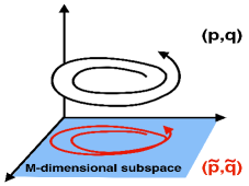
Figure 1: Pictorial representation of the projection procedure.

In few words, a full dimensional classical trajectory (black line) has higher odds to get close to its initial configuration if projected onto a subspace (red line). Based on this observation, we propose that while classical trajectories be still treated in full dimensionality, the semiclassical calculation employ sub-space bounded information to yield projected spectra. From a statistical point of view, the procedure corresponds to the calculation of a marginal distribution in each subspace after marginalizing out the other degrees of freedom.(Trumpler and Weaver, 1962) As a final step, the composition of the several projected spectra provides the full-dimensional one.

We apply this idea to spectral density, $I(E)$, calculations

$$I\left(E\right)\equiv\frac{1}{2\pi\hbar}\int_{-\infty}^{+\infty}\left\langle\chi\left|e^{-i\hat{H}t/\hbar}\right|\chi\right\rangle e^{iEt/\hbar}dt.$$ (1)

An exact representation of the quantum propagator $e^{-i\hat{H}t/\hbar}$ is given by Feynman’s path integral formulation, which can be approximated by considering only the classical paths connecting points ${\bf q}{}_{0}$ and ${\bf q}^{\prime}$ in time t (roots) and including fluctuations up to the second order around the classical action ($S^{cl}$) of each path(Gutzwiller, 1967; Van Vleck, 1928)

$$\left\langle\mathbf{q}^{\prime}\left|e^{-\frac{i}{\hbar}\hat{H}t}\right|\mathbf{q}_{0}\right\rangle\approx\sum_{roots}\left[\dfrac{\left|-\frac{\partial^{2}S_{t}^{cl}}{\partial\mathbf{q}^{\prime}\partial\mathbf{q}_{0}}\right|}{\left(2\pi i\hbar\right)^{N}}\right]^{1/2}\dfrac{e^{\frac{i}{\hbar}S_{t}^{cl}\left(\mathbf{q}^{\prime},\mathbf{q}_{0}\right)}}{e^{i\upsilon\pi/2}}.$$ (2)

Eq. (2) represents the semiclassical approximation to the Feynman path integral.(Berry and Mount, 1972) The term $e^{-i\upsilon\pi/2}$, where $\upsilon$ is the integer Maslov index, ensures the continuity of the square root of the pre-exponential factor. However, the drawback of Eq. (2) is the presence of points at which the determinant in the pre-exponential factor becomes singular. Miller’s SCIVR(Miller, 1970b; Heller, 1991) overcomes this issue by replacing the sum over classical trajectories with an integration over initial momenta, a very powerful approach especially when combined with Heller’s coherent states ($|\mathbf{p},\mathbf{q\rangle}$) representation. Coherent states have a Gaussian coordinate-space representation whose width is given by the (usually diagonal) $\Gamma$ width matrix

$$\left\langle\mathbf{x}|\mathbf{p},\mathbf{q}\right\rangle=\left(\frac{det\left(\Gamma\right)}{\pi^{N}}\right)^{1/4}e^{-\left(\mathbf{x}-\mathbf{q}\right)^{T}\frac{\Gamma}{2}\left(\mathbf{x}-\mathbf{q}\right)+i\mathbf{p}\left(\mathbf{x}-\mathbf{q}\right)/\hbar}.$$ (3)

By using Miller’s SCIVR and by either reformulating the Feynman paths(Weissman, 1982; Baranger et al., 2001) or representing the spectral density $I(E)$(Herman and Kluk, 1984) in terms of the coherent states of Eq. (3), one gets to the working formula

$$I\left(E\right)=\frac{1}{2\pi\hbar}\int_{-\infty}^{+\infty}dte^{iEt/\hbar} \frac{1}{\left(2\pi\hbar\right)^{N}}\int\int d\mathbf{q}_{0}d\mathbf{p}_{0}C_{t}\left(\mathbf{p}_{0},\mathbf{q}_{0}\right)$$ (4)

$$e^{iS_{t}\left(\mathbf{p}_{0},\mathbf{q}_{0}\right)/\hbar}\left\langle\chi|\mathbf{p}_{t},\mathbf{q}_{t}\right\rangle\left\langle\mathbf{p}_{0},\mathbf{q}_{0}|\chi\right\rangle.$$

where

$$C_{t}\left(\mathbf{p}_{0},\mathbf{q}_{0}\right)=\sqrt{\frac{1}{2}\left|\frac{\partial\mathbf{q}_{t}}{\partial\mathbf{q}_{0}}+\frac{\partial\mathbf{p}_{t}}{\partial\mathbf{p}_{0}}-i\hbar\Gamma\frac{\partial\mathbf{q}_{t}}{\partial\mathbf{p}_{0}}+\frac{i}{\Gamma\hbar}\frac{\partial\mathbf{p}_{t}}{\partial\mathbf{q}_{0}}\right|}.$$ (5)

In order to accelerate the Monte Carlo integration of Eq. (4), it is possible to insert a time averaging filter $\frac{1}{T}\int_{0}^{T}dt$ without loss of accuracy by virtue of Liouville’s theorem. Miller et al.(Kaledin and Miller, 2003a, b) worked out the following time averaged (TA) version of Eq. (4)

$$I\left(E\right) = \left(\frac{1}{2\pi\hbar}\right)^{N}\iintop d\mathbf{p}_{0}d\mathbf{q}_{0}\frac{1}{2\pi\hbar T}$$ (6)

$$\times \left|\intop_{0}^{T}dte^{\frac{i}{\hbar}\left[S_{t}\left(\mathbf{p}_{0},\mathbf{q}_{0}\right)+Et+\phi_{t}\right]}\left\langle\bm{\chi}\left|\mathbf{p}_{t}\mathbf{q}_{t}\right.\right\rangle\right|^{2}$$

where the additional approximation $\phi\left(t\right)=\mbox{phase}\left[C_{t}\left(\mathbf{p}_{0},\mathbf{q}_{0}\right)\right]$ has been introduced. Eq. (6) is now much easier to converge due to its positive-definite integrand, and it has been tested on several molecules(Kaledin and Miller, 2003a; Conte et al., 2013b; Ceotto et al., 2011b; Gabas et al., 2017; Ceotto et al., 2011a) yielding very accurate results upon evolution of just about $1000$ trajectories per degree of freedom. The interested reader can find detailed derivations of the above formulae in Ref. 83 (Chapter 10) or in Ref. 84.

To further reduce the computational overhead to just a handful of trajectories we have recently developed an implementation of Eq. (6) based on two observations. First, accurate eigenvalues can be extracted from a single trajectory whose energy not necessarily must be equal to the exact (but unknown) eigenvalue.(De Leon and Heller, 1983) Second, for each spectroscopic peak the most contributing trajectories are those that evolve in the proximity of the vibrational peak energy shell.(Ceotto et al., 2011a) Based on these considerations, we employ a reference state $\left|\chi\right\rangle=\sum_{i=1}^{N_{\text{states}}}\left|\mathbf{p}_{\text{eq}}^{i},\mathbf{q}_{\text{eq}}^{i}\right\rangle$ written as a combination of coherent states placed at the classical phase space points $\left(\mathbf{p}_{\text{eq}}^{i},\mathbf{q}_{\text{eq}}^{i}\right)$. $\mathbf{q}_{\text{eq}}^{i}$ indicates the equilibrium configuration and $\mathbf{p}_{\text{eq}}^{i}$ the corresponding multidimensional momentum. We set $V\left(\mathbf{q}_{\text{eq}}^{i}\right)=0$, and $\mathbf{p}_{\text{eq}}^{i}$ is chosen to be made of harmonically estimated momenta, i.e. $\left(p_{j,\text{eq}}^{i}\right)^{2}/2m=\hbar\omega_{j}\left(n_{j}^{i}+1/2\right)$ for the generic j-th vibrational mode. The set of $\omega_{j}$ is obtained by diagonalizing the Hessian at the equilibrium configuration. In this way, we can approximate Eq. (6) to

$$I\left(E\right)=\frac{1}{\left(2\pi\hbar\right)^{N}}\frac{Re}{\pi\hbar T}\sum_{i=1}^{n_{states}}$$ (7)

$$\left|\int_{0}^{T}dt\left\langle\sum_{i=1}^{n_{states}}\mathbf{p^{i}}_{eq},\mathbf{q^{i}}_{eq}|\mathbf{p}_{t},\mathbf{q}_{t}\right\rangle e^{i\left(S_{t}\left(\mathbf{p}_{eq}^{i},\mathbf{q}_{eq}^{i}\right)+Et+\phi\left(t\right)\right)/\hbar}\right|^{2}$$

where $n_{states}$ classical trajectories are evolved from the initial conditions $\left(\mathbf{p}_{\text{eq}}^{i},\mathbf{q}_{\text{eq}}^{i}\right)$. This approach is called Multiple Coherent TA-SCIVR (MC-SCIVR) (also indicated as MC-TA-SCIVR). MC-SCIVR has been shown to be accurate for systems of complexity up to the glycine molecule (i.e. 24 degrees of freedom).(Gabas et al., 2017)

The main theoretical novelty presented in this Letter is that we re-formulate Eq.(6) on the basis of projected-trajectory information. First, the $N$ dimensional phase space is conveniently partitioned, i.e. $\left(\mathbf{p},\mathbf{q}\right)\equiv\left(p_{1},q_{1,}...,\tilde{p}_{i},\tilde{q}_{i},...,\tilde{p}_{i+M},\tilde{q}_{i+M},...,p_{N},q_{N}\right)$, where we have highlighted a generic M-dimensional subspace ($M<N)$ with tilde variables $\left(\tilde{\mathbf{p}},\tilde{\mathbf{q}}\right)$ (see Fig.(1)). For this purpose, an analysis is performed concerning the off-diagonal values of the Hessian matrix averaged over a full-dimensional classical trajectory with harmonic zero-point energy. Off-diagonal terms that are bigger than a threshold value ($\varepsilon$) correspond to coupled modes and are included in the same subspace. The threshold choice is driven by the trade-off between calculation accuracy and feasibility. On one hand, the smaller the threshold value the smaller the number of neglected interactions and the more accurate the calculation. On the other, the dimensionality of any projected space should not exceed 20-25 degrees of freedom to permit MC-SCIVR calculations in that subspace. Then, we consider that each vector or matrix appearing in Eq.(6) can be exactly projected into each sub-space by means of a singular value decomposition procedure $\mathbf{A}=\mathbf{U}\mathbf{\Sigma}\mathbf{V}$,(Hinsen and Kneller, 2000) and consequently restrict the phase space integration to $\int\int d\mathbf{\tilde{p}}_{0}d\tilde{\mathbf{q}}_{0}$. The M-dimensional coherent state becomes

$$\left\langle\mathbf{\tilde{x}}\left|\mathbf{\tilde{p}}_{t}\mathbf{\tilde{q}}_{t}\right.\right\rangle=\left(\frac{\mbox{det}(\tilde{\Gamma})}{\pi^{M}}\right)^{\frac{1}{4}}e^{-\frac{1}{2}\left(\mathbf{\tilde{x}}-\mathbf{\tilde{q}}_{t}\right)^{T}\mathbf{\tilde{\Gamma}}\left(\mathbf{\tilde{x}}-\mathbf{\tilde{q}}_{t}\right)+\frac{i}{\hbar}\mathbf{\tilde{p}}_{t}^{T}\left(\mathbf{\tilde{x}}-\mathbf{\tilde{q}}_{t}\right),}$$ (8)

where $\widetilde{\mathbf{\Gamma}}=\mathbf{U}\mathbf{U}^{T}\mathbf{\Gamma}\mathbf{U}\mathbf{U}^{T}$ is the projected Gaussian width matrix obtained from the singular-value decomposition matrix ${\bf U}$.(Harland and Roy, 2003) Similarly, $\widetilde{C}_{t}$ is obtained by projecting its monodromy matrix components. The remaining term of Eq.(6) to be projected is $S_{t}.$ While the projection of the kinetic part of the Lagrangian can be obtained exactly, the potential is generally not separable. In an ideal case, $V_{S}\left(\tilde{\mathbf{q}}_{M}\right)$ would be the potential such that, given the initial conditions $\left(\tilde{\mathbf{p}}_{0},\tilde{\mathbf{q}}_{0}\right)$, the M-dimensional trajectory coincides with the projected one. In such a M-dimensional dynamics, the positions in the other degrees of freedom ($\mathbf{q}_{N-M}$) are downgraded to parameters. In practice, we fix these parameters at equilibrium positions, but introduce an external field $\lambda\left(t\right)$ to account for the non-separability of the potential such that

$$V_{S}\left(\tilde{\mathbf{q}}_{M}\right)\equiv V\left(\tilde{\mathbf{q}}_{M};\mathbf{q}_{N_{vib}-M}\right)=V\left(\tilde{\mathbf{q}}_{M};\mathbf{q}_{N_{vib}-M}^{eq}\right)+\lambda\left(t\right).$$ (9)

$\lambda\left(t\right)$ is not known a priori and we adopt the following expression, which makes Eq. (9) exact (within a constant) in the separable potential limit

$$\lambda\left(t\right) = V\left(\tilde{\mathbf{q}}_{M};\mathbf{q}_{N_{vib}-M}\right)-$$ (10)

$$\left[V\left(\tilde{\mathbf{q}}_{M};\mathbf{q}_{N_{vib}-M}^{eq}\right)+V\left(\tilde{\mathbf{q}}_{M}^{eq};\mathbf{q}_{N_{vib}-M}\right)\right].$$

Moving to applications, we have first tested accuracy and effectiveness of our new Divide-and-Conquer Semiclassical Initial Value Representation (DC-SCIVR) approach on three different molecular systems for which exact vibrational eigenenergies are available in the literature.

Water is a low dimensional but strongly coupled system. Its global 3-dimensional vibrational space can be divided into a monodimensional one for the bending mode, plus a bidimensional one for the two stretches. We evolved 3500 classical trajectories on a pre-existing potential energy surface,(Bowman et al., 1988) each one for a total of 30000 atomic time units. The zero point energy (ZPE) estimated from the projected spectra is 4606 $cm^{-1}$, to be compared to the 4631 $cm^{-1}$ value of a full dimensional semiclassical calculation, and the exact quantum value of 4636 $cm^{-1}$. DC-SCIVR reproduces fundamentals concerning the bending and the asymmetric stretch with excellent accuracy (within 10 cm^-1 of exact quantum results), while the symmetric stretch and the first bending overtone are more off the mark (40 cm^-1). Overall, the mean absolute error (MAE) is 23 $cm^{-1}$. Detailed comparisons can be found in the Supplemental Material.(Sup, ) Results for water are a remarkable milestone because of the strong internal vibrational coupling of this molecule. In fact, in higher dimensional systems inter-mode couplings are generally weaker and DC-SCIVR (being exact for separable systems) is expected to perform better once strongly coupled modes are confined into the same subspace.

Table 1: Vibrational frequencies of CH₄. “QM” labels the exact quantum eigenvalues; “SCIVR” refers to a full dimensional semiclassical calculation; “DC-SCIVR” labels frequencies obtained with the “divide-and-conquer” approach here presented; “HO” are harmonic estimates. All values are in $cm^{-1}.$

State	QM(Carter et al., 1999)	SCIVR	DC-SCIVR	HO
$1_{1}$	1313	1300	1300	1345
$2_{1}$	1535	1529	1532	1570
$1_{2}$	2624	2594	2606	2690
$1_{1}2_{1}$	2836	2825	2834	2915
$3_{1}$	2949	2948	2964	3036
$2_{2}$	3067	3048	3050	3140
$4_{1}$	3053	3048	3044	3157
MAE		12	11	68

Another known issue for SC methods comes from chaotic trajectories which can spoil the SC simulation and are therefore usually discarded. In an application of DC-SCIVR to methane, the 9-dimensional vibrational space has been partitioned into a 6-dimensional and a 3-dimensional one and it turns out that methane dynamics is highly chaotic with strong quantum effects, given the light mass of the hydrogen atoms. In fact, 95% of the 180000 trajectories run (each one evolved for 30000 atomic time units) has been discarded on the basis of the monodromy determinant conservation criterion.(Kaledin and Miller, 2003b; Zhuang et al., 2012) Table 1 provides a comparison between our DC-SCIVR estimates and exact values by Bowman on the same analytical surface.(Carter et al., 1999) This test permits to show that DC-SCIVR works pretty well, with fundamentals and overtones reliably detected and a tiny MAE (11 cm^-1).

Recently, by employing a pre-existing potential energy surface,(Maslen et al., 1992) Halverson and Poirier have calculated a set of quantum vibrational frequencies of benzene with their exact quantum dynamics (EQD) method,(Halverson and Poirier, 2015) which we use to benchmark our DC-SCIVR results for this high dimensional molecular system. For this purpose, the vibrational space of benzene has been divided into a larger 8-dimensional subspace plus 8 bidimensional and 6 monodimensional ones. We have evolved 1,000 trajectories per degree of freedom for a total of 30000 atomic time units each. Furthermore, an accurate second-order perturbative approximation to the pre-exponential factor $\exp(i\phi(t)/\hbar)$, as described in Ref. 71, has been employed to avoid discard of chaotic trajectories. Results are reported in Table 2 and permit to assess DC-SCIVR accuracy in this challenging application. Even in the case of benzene DC-SCIVR is characterized by a small MAE value (19 cm^-1). This is the result of a large majority of highly accurate frequencies and a single mode with lower precision.

Table 2: Comparison between DC-SCIVR and available quantum results (EQD) for benzene fundamental frequencies. Degenerate frequencies are not replicated. Values are in $cm^{-1}.$

State	DC-SCIVR	EQD(Halverson and Poirier, 2015)	State	DC-SCIVR	EQD(Halverson and Poirier, 2015)
11	388	399.4554	101	1024	1040.98
21	610	611.4227	111	1157	1147.751
31	732	666.9294	121	1157	1180.374
41	706	710.7318	131	1295	1315.612
51	908	868.9106	141	1357	1352.563
61	990	964.0127	151	1460	1496.231
71	996	985.8294	161	1606	1614.455
81	996	997.6235
91	1018	1015.64	MAE	19

Finally, after having benchmarked the accuracy of our method against exact quantum results for three molecules of different dimensionality and complexity, we demonstrate applicability of DC-SCIVR to an extremely high dimensional problem by computing the power spectrum of a fullerene-like system. $\text{C}{}_{60}$ has 174 vibrational degrees of freedom, a number which makes a fully quantum mechanical calculation as well as a standard semiclassical simulation clearly unfeasible and calls for an efficient alternative method. We employed a pre-existing force field derived from DFT calculations on graphene sheets. This force field takes into account stretching, bending, and torsional contributions, but neglects bond-coupling terms and van der Waals interactions.(Holec et al., 2010) It is therefore not tailored on a real fullerene molecule, but the main intent of this final application is to show that our method can overcome the “curse of dimensionality” even in very challenging instances. DC-SCIVR starts off with the definition of the subspaces in which the projected spectra must be computed. Fig (2) shows how the choice of the threshold influences the maximum subspace dimensionality for this system. As previously anticipated, a trade-off leads to considering only instances within the dashed blue lines. On the basis of Fig (2), we have chosen a threshold value of $10^{-6}$, which corresponds to a maximum subspace dimensionality equal to 25. This choice has permitted to divide the 174-dimensional vibrational space into 90 monodimensional, 1 bidimensional, 3 three-dimensional, 2 six-dimensional, 1 eight-dimensional, two 14-dimensional, and one 25-dimensional subspaces. To calculate the projected spectra we ran $175$ classical trajectories, each one evolved for 50000 atomic time units. We employed a reference state $\left|\chi\right\rangle$ selected in agreement with the previously described MC-SCIVR recipe, and, as in the case of benzene, a second-order perturbative approximation to the pre-exponential factor. Figure (3) reports, as an example, the DC-SCIVR spectrum of one of the subspaces. We have also simulated and plotted a transient full dimensional classical spectrum on the basis of the same trajectories employed for the semiclassical calculations. To better compare the two different simulations we have shifted the DC-SCIVR spectrum in such a way that the zero-point energy is set to zero. From the comparison, we note that DC-SCIVR and classical estimates are close to each other. However, DC-SCIVR is able to increase the level of knowledge by detecting also quantum overtones. Results up to an energy of about 1600 cm^-1 relative to the zero point energy can be found in Table (3).

Table 3: Frequencies of the C₆₀ model up to 1600$cm^{-1}$. “HO” indicates harmonic values; “Cl” labels the classical estimates of fundamental frequencies; “DC-SCIVR” introduces our semiclassical results. Values are in $cm^{-1}.$

State	HO	Cl	DC-SCIVR	St.	HO	Cl	DC-SCIVR	St.	HO	Cl	DC-SCIVR	St.	HO	Cl	DC-SCIVR	St.	HO	Cl	DC-SCIVR
$1_{1}$	255	254	254	$10_{1}$	568	611	610	$5_{2}$	808		807	$23_{1}$	1014	1015	1015	$29_{1}$	1310	1269	1264
$2_{1}$	318	355	352	$11_{1}$	601	571	572	$17_{1}$	816	779	774	$24_{1}$	1042	1039	1037	$13_{2}$	1314		1303
$3_{1}$	359	347	346	$2_{2}$	636		706	$18_{1}$	863	872	872	$25_{1}$	1052	1075	1075	$31_{1}$	1457	1438	1434
$4_{1}$	404	432	432	$12_{1}$	648	630	626	$19_{1}$	890	911	911	$26_{1}$	1091	1062	1060	$32_{1}$	1470	1398	1391
$5_{1}$	404	404	403	$13_{1}$	657	652	651	$20_{1}$	905	880	880	$9_{2}$	1092		1091	$33_{1}$	1526	1467	1506
$6_{1}$	484	483	483	$3_{2}$	718		693	$21_{1}$	962	971	971	$10_{2}$	1136		1220	$14_{2}$	1540		1534
$7_{1}$	488	547	547	$14_{1}$	770	767	767	$6_{2}$	968		966	$11_{2}$	1202		1150	$15_{2}$	1550		1533
$8_{1}$	494	478	478	$15_{1}$	775	766	766	$7_{2}$	976		1093	$27_{1}$	1225	1218	1218	$16_{2}$	1562		1554
$1_{2}$	510		506	$16_{1}$	781	777	777	$8_{2}$	988		957	$28_{1}$	1252	1231	1231
$9_{1}$	546	545	546	$4_{2}$	808		863	$22_{1}$	1000	997	998	$12_{2}$	1296		1254

A concern that may arise about the approach regards its efficiency when dealing with lower-symmetry molecules. Thus, to demonstrate that reduced symmetry is not a hindrance to our calculations, we have investigated an ad hoc constructed fullerene isotope model for which symmetry has been broken. Substitution of three appropriate carbon nuclei with nuclei having the same mass of gold ones removed the degeneracies of the vibrational levels. This model was built to preserve the original nuclear and electronic charges, so that the force field did not need to be modified.
The result of the isotopic substitution is that previously degenerate frequencies are split already at the harmonic level. Even if such splittings are mostly within semiclassical accuracy (i.e. 25-30 cm^-1), DC-SCIVR results are resolved enough to detect a multiple-peak feature in the isotopic model opposite to the original case characterized by a lonely (degenerate) peak. A relevant example of this is reported in the Supplemental Material.(Sup, )

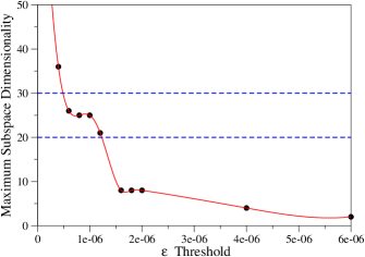
Figure 2: Maximum subspace dimensionality vs threshold $\varepsilon$ for the C₆₀ calculation. The red curve fits the overall behavior, while the dashed blue lines define the range of desired maximum subspace dimensionality.

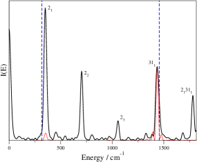
Figure 3: DC-SCIVR (black line) and classical (red line) spectra for one of the subspaces employed in the C₆₀ calculation. Harmonic frequencies are reported in dashed blue lines. Labels are according to Table (3).

In summary, we have presented a new approach to the calculation of theoretical vibrational spectra of high dimensional molecular systems. The method has been tested for the small and highly inter-mode coupled water molecule, the highly chaotic methane molecule, and the high dimensional benzene molecule yielding in all cases accurate estimates if compared to available exact quantum results. Then, application to a sizable system made of 174 degrees of freedom has demonstrated that even for such large systems an accurate quantum estimate of fundamental and overtone frequencies is feasible, thus opening up the possibility to quantum investigate the spectroscopy of highly dimensional systems.