Transition to reconstructibility in weakly coupled networks

Abstract

Across scientific disciplines, thresholded pairwise measures of statistical dependence between time series are taken as proxies for the interactions between the dynamical units of a network. Yet such correlation measures often fail to reflect the underlying physical interactions accurately. Here we systematically study the problem of reconstructing direct physical interaction networks from thresholding correlations. We explicate how local common cause and relay structures, heterogeneous in-degrees and non-local structural properties of the network generally hinder reconstructibility. However, in the limit of weak coupling strengths we prove that stationary systems with dynamics close to a given operating point transition to universal reconstructiblity across all network topologies.

Introduction

Complex networked systems generate dynamics and thus function that fundamentally depend on how their units interact [1, 2, 3]. As a consequence, knowing the interaction topology of such systems is a key towards understanding them [4, 5, 6, 7, 8, 9, 10, 11, 12]. Yet, direct access to the topology of physical interactions is largely limited for many natural systems and across scales, ranging from metabolic and gene regulatory networks on the subcellular level to neural circuits of millions of cells, to food webs among organisms and planetary climate networks [13, 10, 14, 15, 16, 17, 18, 19, 20, 21]. Thus, measures of pairwise statistical dependencies between time series of the dynamics of their units are often employed as proxies for physical interactions [15, 22, 23, 24, 17, 25, 26, 21, 16, 27]. Assuming sufficiently many and sufficiently accurate data, each such method provides useful information about how the considered statistical dependency measures vary across pairs of units. The value of such a statistical measure, thresholded as desired, e.g. for significance against coincident correlations, may be taken to quantify the interactions among these units. Yet, such measures themselves do not necessary provide immediate insights into how the units are directly influencing each other via physical interactions. In particular, what do correlations generally tell us about direct physical interactions in network dynamical systems? And is it possible to detect direct physical interactions among units by thresholding these measures to reconstruct the topology of the network?

Here, we systematically address this question on a conceptual level and identify limits of network reconstructibility based on thresholding pairwise measures of statistical dependence. In general, non-linearities of intrinsic and coupling dynamics, correlated noise sources, heterogeneities in time scales and coupling strengths as well as nontrivial network topology jointly create complex statistical correlation patterns. To reveal principal limits of reconstructibility originating from network interactions (toplogy and strength), we here focus on systems with dynamics around a given operating point. More specifically, we analyze the idealized setting of linearly coupled systems with homogeneous dynamical parameters receiving independent additive noise inputs and evaluate network reconstruction from thresholding linear correlations obtained from sufficiently long time series. Reconstruction of physical interactions generally is at least as hard in any more complex setting, e.g., involving non-linear dynamics and adequate measures of statistical dependence such as mutual information. We explicate limits of reconstructibility due to local common cause structures, local relay structures, topological in-degree heterogeneities as well as non-local structural elements. Despite these limitations our analysis interestingly also reveals that, stationary systems close to operating points exhibit a transition to universal reconstructibility for sufficiently weak coupling, independent of the interaction topology.

Model and Methods

Consider the dynamics

$$\tau_{\text{gl}}\dot{x}_{i}=-x_{i}+\alpha\sum_{j=1}^{N}A_{ij}(x_{j}-x_{i})+\gamma\eta_{i}(t)$$ (1)

of network dynamical systems characterized by variables $\mathbf{x}=(x_{1},\ldots,x_{N})$ that interact diffusively with generic coupling strength $\alpha>0$ on a network topology given by an adjacency matrix $A$. The units are driven by independent white noise $\eta_{i}(t)$ of strength $\gamma$ and relax on a time scale $\tau_{\text{gl}}>0$. The entries of the weighted adjacency matrix are $A_{ij}>1$ if unit $j$ physically acts on $i$, with all other elements, including the diagonal being $A_{ij}=0$. Without loss of generality, we rescale time such that $\tau_{\text{gl}}=1$. This dynamics characterizes linear systems as well as stationary systems sufficiently close to given operating points.

Figure 1: (color online) Topology-induced limits of reconstructibility. Reconstructing interaction networks from correlation thresholding may or may not yield correct connectivity pattern. (a)-(d) Successful reconstruction of a network ($N=15$, average degree $\bar{k}=5$, $\gamma=1$, $\alpha=2,A_{ij}\in\{0,1\}$ for absent and present interactions, resp.). (e)-(h) Reconstruction of statistically similar network is unsuccessful for any threshold. (a,e) Adjacency matrix of original network (black indicated directed interaction, gray undirected network aimed for). (b,f) Dynamics of the units yielding (c,g) correlation matrices. Thresholding yields (d) correct or (h) incorrect reconstruction, depending on the exact topology.

Can we infer the physical topology from optimally thresholding the matrix $C$ of pairwise correlations (Fig. 1)? The covariance matrix $\sigma$ defined by the elements

$$\sigma_{ij}=\langle x_{i}x_{j}\rangle-\langle x_{i}\rangle\langle x_{j}\rangle$$ (2)

computed using an unbiased time-average $\langle\cdot\rangle$, yields the correlations

$$C_{ij}=\frac{\sigma_{ij}}{\sqrt{\sigma_{ii}\sigma_{jj}}}$$ (3)

by normalization.

Reconstructing the physical topology implies detecting non-zero elements in the coupling matrix $A$. Also, as correlation matrices are symmetric by construction, $C_{ij}=C_{ji}$, we relax the problem to the reconstruction of the undirected representation of the physical interaction network. Thus, we aim for the correct reconstruction of the matrix $A^{\prime}$ the elements of which are given by

$$A^{\prime}_{ij}=\begin{cases}1&\textrm{if}\;A_{ij}=1\textrm{ or }A_{ji}=1\\ 0&\textrm{otherwise}\end{cases}$$ (4)

Correlations (3) may be thresholded using a (possibly optimized) threshold $\theta$ to yield an estimate $\hat{A^{\prime}}$ with elements $\hat{A^{\prime}}_{ij}=1$ if $C_{ij}>\theta$ and $\hat{A^{\prime}}_{ij}=0$ otherwise. Below we focus on the question whether there is any threshold of the correlation matrix (3) that yields a correct estimate of $A^{\prime}$. If there is no such threshold, we call the network non-reconstructible (in this sense).

The theory of Ornstein-Uhlenbeck processes [28] yields an analytical expression for the covariance matrix

$$\sigma=\gamma^{2}\int_{0}^{\infty}e^{Jt}e^{J^{\textsf{T}}t}\;\text{d}t.$$ (5)

Here, the matrix $J$ is given by its elements

$$J_{ij}=\begin{cases}-(1+\alpha\sum_{j=1}^{N}A_{ij})&\text{if }i=j\\ \alpha A_{ij}&\text{otherwise}.\end{cases}\;$$ (6)

Partial integration of (5) yields the Lyapunov equation

$$J\sigma+\sigma J^{\text{T}}+\gamma^{2}I=0$$ (7)

which we solve numerically [29] to obtain the covariance matrix $\sigma$ for arbitrary $(\alpha,\gamma,A)$. Via the relation (3), we thus semi-analytically obtain all the real-valued elements $C_{ij}$ of the correlation matrix without any sampling error. We order those to determine whether there is a threshold $\theta$ separating all existing from all non-existing links.

Results

Topology-induced limits of reconstructibility.

Even under these idealized conditions, physical interactions are in general not reconstructible from thresholding the correlation matrix $C$. Whereas some topologies can be reconstructed via a threshold that separates existing from absent links (Fig. 1a-d), many attempted reconstructions yield false positive and false negative predictions of links, independent of the threshold (Fig. 1e-f) and are thus intrinsically non-reconstructible by correlation thresholding.

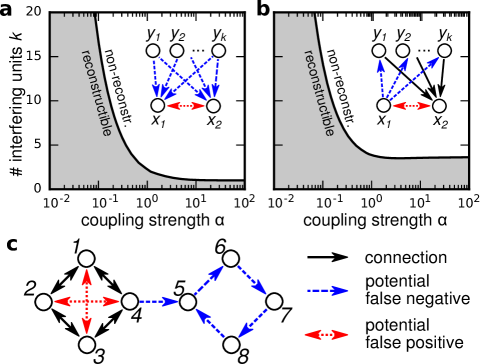
Figure 2: (color online) Topological sources of reconstruction errors and impact of coupling strenghts. (Unspecified parameters as in Fig. 1) (a,b) Regions of reconstructible (shaded gray) and non-reconstructible networks (white shading) are non-linearly separated for (a) common cause structures and (b) relay structures. (Regimes computed by interpolating analytic results using (3) and (5).) (c) Non-local effect renders larger networks non-reconstructible: Each circle would be reconstructible alone, but the joint network is not ($\alpha=2$).

Topologically induced errors and ultimately the limits in reconstructibility can be of local or of non-local nature (Fig. 2): For instance, common input might cause unconnected units to be more correlated than connected units, a dilemma known as the common cause effect (Fig. 2a inset). Likewise, two units may be strongly correlated if the network provides connectivity between them across a set of intermediate units, thereby forming a relay structure (Fig. 2b inset). For both settings, reconstructibility non-linearly depends on a combination of overall coupling strength and the number of interfering units in a systematic way (Fig. 2a,b, main panels).

In larger networks with diameter $d\geq 3$, additional non-local effects limit reconstructibility (illustrated in Fig. 2c). Differences in the correlation strength may, for instance, be caused by different link densities in different parts of the network, and imply incorrect link classification.

Figure 3: Transition to reconstructibility for weak coupling. (a) Correlation thresholding yields different estimators (shaded areas with graphs as insets) for a given topology (adjacency matrix on bottom right) depending on coupling strength and threshold. For sufficiently small coupling strength $\alpha$ (left of gray dashed line), there are ideal thresholds yielding perfect reconstruction (green shading). (Analytic results obtained using (3) and (5).) (b) Fraction of reconstructible networks exhibits transition to full reconstructibility at positive coupling strength $\alpha$ (inset) and $\alpha N$ (main panel), illustrated for random networks of $N\in\{16,64,256\}$ units and link probability $p=0.5$. Every arbitrary network exhibits such a transition individually (see text).

Universal transition to non-reconstructibility.

The coupling strength $\alpha$ controls the impact of both, local and non-local influences on reconstructibility. For instance, analytic treatment of a small common cause structure (Fig. 3) reveals that the system becomes reconstructible for all sufficiently small coupling strengths $\alpha$ while it is non-reconstructibility if $\alpha$ is too large. This systematic transition prevails for any number of common input units in common cause structures as well as for any number of relay units in relay structures (See Supplementary material for detailed derivations).

Interestingly, all topology-induced limits disappear for sufficiently weak coupling, as seen from the following analytic argument: Rewriting the matrix

$$J=-(\mathbb{1}+\alpha L)$$ (8)

in terms of the graph Laplacian $L$ with elements

$$L_{ij}=-A_{ij}+\delta_{ij}\sum_{j}A_{ij}$$ (9)

(where $\delta_{ij}=1$ if $i=j$ and zero otherwise is the Kronecker-delta) and expanding (5) for $\alpha\ll 1$ yields

$$\begin{split}\sigma=\frac{\gamma^{2}}{2}&\left[\mathbb{1}-\frac{\alpha}{2}(L+L{{}^{\intercal}})\right.\\ &+\left.\frac{\alpha^{2}}{2}\left(LL{{}^{\intercal}}+\frac{L^{2}+L{{}^{\intercal}}^{2}}{2}\right)\right]+\mathcal{O}(\alpha^{3})\;.\end{split}$$ (10)

The term $\alpha(L+L{{}^{\intercal}})/2$ on the r.h.s. of (10) does only contribute to entries $\sigma_{ij}$ that reflect existing links because otherwise $L_{ij}=A_{ij}=0$. Thus, the covariance of coupled units scales linearly with $\alpha$ whereas for uncoupled units it scales quadratically. So for sufficiently small coupling strength $\alpha$, covariances of coupled units will be larger than those of uncoupled units. This result transfers to the elements of the correlation matrix $C$ in (3) because diagonal elements of the covariance matrix $\sigma$ are of order

$$\sigma_{ii}=\mathcal{O}(\alpha^{0})\textrm{ as }\alpha\rightarrow 0.$$ (11)

Hence, every network topology is reconstructible for sufficiently small coupling strengths.

Illustrative example of reconstructibility transition.

Furthermore, specific families of networks with homogeneous connectivity are reconstructible via correlation thresholding for all coupling strengths, weak and strong.

As we demonstrate for illustration, this is the case for directed ring like topologies with $\bar{k}$ neighbors. In these networks the correlation matrix $C$ is strictly proportional to the covariance matrix $\sigma$ so that it is sufficient to show reconstructibility with respect to the covariance matrix. Also, since the covariance matrix $\sigma$ is a circulant, it is sufficient to show reconstructibility only for the connections of one unit. The reconstructibility conditions is identical for all units. For simplicity of presentation, we take the number $N$ of units to be even.

We order the units in such a way that it reflects the network topology, i.e.

$$A_{i,(i+l)\operatorname{mod}N}=\begin{cases}1&\textrm{if}\;1<l\leq\bar{k}\\ 0&\textrm{otherwise}\end{cases}\;,$$ (12)

and replace $J=-(\mathbb{1}+\alpha A)$ in Eq. (7) to obtain

$$\sum\limits_{l=1}^{\bar{k}}\sigma_{i,i+n-l}-2\frac{\alpha+{\bar{k}}}{\alpha}\sigma_{i,i+n}+\sum\limits_{l=1}^{\bar{k}}\sigma_{i,i+n+l}=-\frac{\gamma^{2}}{\alpha}\delta_{i,i+n}\;$$ (13)

for the covariance matrix $\sigma$. Here, the index $i$ indicates the number of the unit and is thus arbitrary.

Transforming this equation into Fourier space yields

$$\sum_{l=1}^{k}e^{-2\pi i\frac{lm}{N}}s_{m}-2(\frac{1}{\alpha}+k)s_{m}+\sum_{l=1}^{k}e^{2\pi i\frac{lm}{N}}s_{m}=-\frac{\gamma^{2}}{\alpha}$$ (14)

with solution

$$s_{m}=\frac{\gamma^{2}}{\alpha}\frac{1}{2(\frac{1}{\alpha}+k)-2\sum\limits_{l=1}^{k}\cos\left(2\pi\frac{lm}{N}\right)}$$ (15)

in Fourier coordinates. An inverse Fourier transformation yields the analytic solution

$$\sigma_{i,i+n} =\frac{\gamma^{2}}{2+2\alpha\bar{k}+\alpha}\left\{\delta_{0n}+\sum_{l=1}^{\infty}\frac{\alpha^{l}\zeta_{{\bar{k}},n}^{\ast l}}{(2+2\alpha\bar{k}+\alpha)^{l}}\right\}$$ (16)

where the sequences $\zeta_{{\bar{k}},n}^{\ast l}$ are repeated convolutions of the step sequence

$$\zeta_{\bar{k},n} =\begin{cases}1&\text{if}\quad n\!\!\!\mod\!N\leq\bar{k}\\ 1&\text{if}\quad N-\bar{k}\leq n\!\!\!\mod\!N\\ 0&\text{otherwise}\end{cases}\;,$$ (17)

i.e.,

$$\begin{aligned} \zeta_{\bar{k}}^{\ast l}:&=(\zeta_{\bar{k}}\ast\zeta_{\bar{k}}^{\ast(l-1)})\;,&\zeta_{\bar{k}}^{\ast 1}&=\zeta_{\bar{k}}\;.\end{aligned}$$ (18)

Since the sequences $\zeta_{\bar{k},n}^{\ast}$ are monotonically decreasing in the interval $n\in[-N/2,N/2]$ covariance only decreases with distance in the circular graph. Because for any given unit $i$, connected units are closer than non-connected units, for every such network with $k$-regular topology, a threshold exists that separates existing from absent links, making these networks reconstructible for arbitrary coupling strengths, for any network size $N$ and for any number of neighbors $\bar{k}<\frac{N}{2}$. For $\bar{k}=\frac{N}{2}$ the undirected representation of the network is fully connected and reconstruction is trivial.

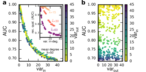
Figure 4: (color online) Reconstruction systematically varies with heterogeneities in in-degree, but not in out-degree. (a) AUC exhibits functional dependency on the variance of the in-degree distribution $\textrm{var}_{\textrm{in}}$, regardless of the variance of the out-degree $\textrm{var}_{\textrm{out}}$. Inset: Qualitative behavior is the same for differnet mean degrees. (b) No significant dependency of reconstruction quality on out-degree heterogeneity (network size $N=150$ throughout, $\alpha=1$, $A_{ij}\in\{0,1\}$).

Which heterogeneities hinder reconstruction?

Given the insights from the ring-like networks, we hypothesized that if topological irregularities increase, they decrease and ultimately hinder network reconstructibility. To analyze the overall impact of topology on reconstruction quality, we investigated ensembles of directed networks in the regime between regular and random, employing a modified Watts-Strogatz small world model [30]: Starting with a regular ring of $N$ units with each unit receiving directed links from $\bar{k}$ preceding nodes, the source and the target of each link are detached with probability $q_{\text{out}}$ and probability $q_{\text{in}}$ respectively. The resulting loose ends are randomly redistributed in the network while avoiding self-loops and multiple links. This creates networks of mean degree $\bar{k}$ whose in-degree distribution $p^{\text{in}}_{k}$ and out-degree distribution $p^{\text{out}}_{k}$ are altered separately from their original values $p^{\text{in}}_{k}=p_{k}^{\text{out}}=\delta_{k\bar{k}}$ by varying $q_{\text{in}}$ and $q_{\text{out}}$. This random graph ensemble contains networks with unimodal degree distributions (binomial for $q_{\text{in}}=q_{\text{out}}=1$, $\bar{k}\ll N$ and $1\ll N$) so that the variances of the distributions serve as indicators for the inhomogeneities in the network.

Considering a fixed coupling strength (e.g., $\alpha=1$), we quantify reconstructibility by measuring the AUC, the area under the ROC (receiver operating characteristic) curve, generated by a variable correlation threshold $\theta$. AUC ranges from AUC=0.5 for random guessing to AUC=1 for perfect reconstructibility (see Supplemental Information for an introduction to ROC curves). For networks that are not densely connected ($\bar{k}<(N-1)/2$), we find that reconstruction quality systematically decreases with in-degree heterogeneity, with the AUC exhibiting a functional dependency on the variance of the in-degree distribution, yet is almost independent of the variance of the out-degree distribution (compare Fig. 4a with Fig. 2b). Thus, the reconstruction error is mainly explained by the in-degree heterogeneity. We obtain qualitatively similar results across different average connectivities $\bar{k}$ (inset of Fig. 4a).

Conclusions

In summary, we have systematically investigated reconstructibility of physical interaction networks from thresholding statistical correlations. Beyond valuable previous studies which targeted the impact of correlated noise and estimation errors [31, 32], we revealed intrinsic limits of reconstructibility induced by the strengths of network interactions and their topology. In particular, a number of distinct topological factors contribute in a systematic way: local common cause structures, local relay structures, in-degree heterogeneities as well as non-local structural elements of a network resulting from different link densities in different network parts. Intriguingly, for stationary dynamics and arbitrary network topologies we uncovered a transition to full reconstructibility when decreasing the coupling strengths. Whereas the exact critical coupling strength to transition to reconstructibility depends on the topology, it is guaranteed to occur for all topologies.

Given the limitations of correlation thresholding, alternate methods of reconstruction from time series data are required. For systems that are strongly non-linear and non-stationary, the range of inference methods is currently largely limited to systems with models known a priori. Such non-linear systems in general pose a number of additional challenges, including that there typically is no well-defined, temporally constant coupling strength between the units. Future studies would need to investigate model-independent methods to obtain physical interaction structure from recorded non-linear dynamics [4, 5, 6, 7, 8, 9, 10, 11, 12]. Our main result on full reconstrucatbility in the weak coupling limit might provide a useful initial step towards the reconstruction of non-linear and non-stationary networks: By systematically combining localized but faithful reconstructions obtained from an entire set of dynamics around different operation points in weakly coupled networks a global picture of the underlying interactions and their network state-dependencies could be obtained.

Our results on topology-induced limits of network reconstructibilty not only further our theoretical insights about the relations between statistical correlation and physical interaction networks [23, 24, 33] but also indicate where principal care has to be taken in applications when analyzing statistical correlation data to reveal aspects of direct physical interactions.

*

Appendix A Model

Here, we consider networks of $N$ units each described by a state variable $x_{i}$, $i\in\{1,\ldots,N\}$, that evolve according to an Ornstein-Uhlenbeck (OU) process given by

$$\dot{x_{i}}=-x_{i}+\alpha\sum\limits_{j=1}^{N}A_{ij}(x_{j}-x_{i})+\gamma\eta_{i}(t)\;$$ (19)

with $\boldsymbol{\dot{x}},\boldsymbol{x}\in\mathbb{R}^{N}$, white noise vector $\boldsymbol{\eta}(t)\in\mathbb{R}^{N}$, adjacency matrix $A_{ij}\in\{0,1\}^{N\times N}$, coupling strength $\alpha\in\mathbb{R_{+}}$ and noise strength $\gamma\in\mathbb{R}_{+}$.

Introducing the Laplace matrix $L$ with elements

$$L_{ij}=-A_{ij}+\delta_{ij}\sum\limits_{k=1}^{N}A_{ik}$$ (20)

(where $\delta_{ij}$ is the Kronecker-delta) and the drift matrix

$$J=-(\mathbb{1}+\alpha L)$$ (21)

the process (19) can be rewritten in the multivariate form

$$\dot{\boldsymbol{x}}=J\boldsymbol{x}+\gamma\boldsymbol{\eta}(t).$$ (22)

Since the drift matrix $J$ is diagonally negative dominant, it has only eigenvalues with non-zero negative real part, so that the process has a stationary solution with covariance matrix

$$\sigma =\gamma^{2}\int\limits_{0}^{\infty}e^{Jt}e^{J{{}^{\intercal}}t}\;\text{d}t$$ (23)

that fulfills the Lyapunov equation

$$J\sigma+\sigma J{{}^{\intercal}}+\gamma^{2}\mathbb{1}=0\;.$$ (24)

For reference see [28].

The existence of an analytic equation for the covariance matrix $\sigma$ enables us to compute the covariance matrix directly without simulating the process, avoiding additional errors induced by finite time series.

Appendix B Detailed Analytic Derivation of Correlations

Here, we present the detailed analytic derivation of the analytic correlations in the generalized common cause problem and the generalized relay structure problem.

We proceed as follows:
First, we compute the instantaneous covariance matrix $\sigma$ of the OU process by solving the integral given by (23), or more precisely

$$\sigma=\frac{\gamma^{2}}{\alpha}\int\limits_{0}^{\infty}e^{-\frac{2}{\alpha}t^{\prime}}\underbrace{e^{-Lt^{\prime}}e^{-L{{}^{\intercal}}t^{\prime}}}_{=:\Lambda(t^{\prime})}\;\text{d}t^{\prime}\;.$$ (25)

For this purpose, we calculate the matrix $\Lambda(t)$, which is determined by the topology, and integrate element-wise to get elements of the matrix $\sigma$.
Then, we compute the Pearson correlation matrix $C$ using its definition $C_{ij}=\frac{\sigma_{ij}}{\sqrt{\sigma_{ii}\sigma_{jj}}}$.

For Fig. 2a,b in the manuscript, we then calculate the difference in correlation for existing connections and non-existing connections as a function of coupling strength $\alpha$ and number of source units (common cause problem) $m$ or transmitting units (relay structure) $m$ and interpolate the zero-crossing of this difference in $\alpha$-$m$ space numerically.

B.1 Common Cause Structure

Let $\boldsymbol{Y}=(Y_{1},Y_{2},\ldots,Y_{m})\in\mathbb{R}^{m}$, $\boldsymbol{X}=(X_{1},X_{2})\in\mathbb{R}^{2}$ be two vectors of unit representing random variables and let each element of $\boldsymbol{Y}$ be a source unit of each element of $\boldsymbol{X}$. Then, the topology $A$ and the Laplacian $L$ for the network of the process $\boldsymbol{Z}=(\boldsymbol{X},\boldsymbol{Y)}$ are given by

$$A=\begin{pmatrix}0&0&1&1&\cdots\\ 0&0&1&1&\cdots\\ 0&0&0&0&\cdots\\ \vdots&\vdots&\vdots&\vdots&\ddots\end{pmatrix}\quad\Rightarrow\quad L=\begin{pmatrix}m&0&-1&-1&\cdots\\ 0&m&-1&-1&\cdots\\ 0&0&0&0&\cdots\\ \vdots&\vdots&\vdots&\vdots&\ddots\end{pmatrix}\;.$$ (26)

The matrix power of $L$ yields

$$L^{n}=\begin{cases}m^{n-1}L&n\neq 0\\ \mathbb{1}&n=0\end{cases}\quad n\in\mathbb{N}\;.$$ (27)

Thus, the matrix exponential is given by

$$e^{-Lt} =\sum_{n=0}^{\infty}\frac{(-t)^{n}}{n!}L^{n}$$

$$=\mathbb{1}+\sum\limits_{n=1}^{\infty}\frac{(-t)^{n}m^{n-1}}{n!}L$$

$$=\mathbb{1}+\frac{e^{-mt}-1}{m}L\;.$$ (28)

Hence,

$$\Lambda(t):=e^{-Lt}e^{-L{{}^{\intercal}}t} =\mathbb{1}+\frac{e^{-mt}-1}{m}(L+L{{}^{\intercal}})+\left(\frac{e^{-mt}-1}{m}\right)^{2}LL{{}^{\intercal}}\;$$ (29)

with

$$LL^{T}=\begin{pmatrix}m^{2}+m&m&0&\cdots\\ m&m^{2}+m&0&\cdots\\ 0&0&0&\cdots\\ \vdots&\vdots&\vdots&\ddots\end{pmatrix}\;,$$ (30)

so that the entries of $\Lambda$ are given by

$$\Lambda_{11} =\Lambda_{22}=1+2(e^{-mt}-1)+\frac{m^{2}+m}{m^{2}}(e^{-mt}-1)^{2}$$ (31)

$$\Lambda_{33} =\ldots=\Lambda_{NN}=1$$ (32)

$$\Lambda_{12} =\frac{(e^{-mt}-1)^{2}}{m}$$ (33)

$$\Lambda_{13} =\ldots=\Lambda_{1N}=\Lambda_{23}=\ldots=\Lambda_{2N}=\Lambda_{13}=-\frac{e^{-mt}-1}{m}\;.$$ (34)

All remaining entries not defined by $\Lambda=\Lambda{{}^{\intercal}}$ are zero.
Integrating

$$\sigma_{ij}=\frac{\gamma^{2}}{\alpha}\int\limits_{0}^{\infty}e^{-\frac{2}{\alpha}t}\Lambda_{ij}(t)\;\text{d}t$$ (35)

yields

$$\sigma_{11} =\sigma_{22}=\gamma^{2}\frac{\alpha^{2}m+\alpha m+2}{(\alpha 2+2)(2\alpha m+2)}$$ (36)

$$\sigma_{33} =\ldots=\sigma_{NN}=\frac{\gamma^{2}}{2}$$ (37)

$$\sigma_{12} =\gamma^{2}\frac{\alpha^{2}m}{(\alpha m+2)(2\alpha m+2)}$$ (38)

$$\sigma_{13} =\ldots=\sigma_{1N}=\sigma_{23}=\ldots=\sigma_{2N}=\sigma_{13}=\frac{\gamma^{2}}{2}\frac{\alpha m}{\alpha m+2}\;.$$ (39)

Normalizing yields two different correlation values: The correlation

$$C_{xx} =\frac{\alpha^{2}m}{\alpha^{2}m+\alpha m+2}$$ (40)

of the non-connected nodes $X_{1}$ and $X_{2}$ and the correlation

$$C_{xy} =\sqrt{\left(\frac{\alpha m+2}{\alpha m+4}\right)\left(\frac{\alpha^{2}}{\alpha^{2}m+\alpha m+2}\right)}$$ (41)

for connection from units in $\boldsymbol{Y}$ to units in $\boldsymbol{X}$.

For Fig. 2a of the main article, we determined the difference between correlations of unconnected pairs and connected pairs $C_{xx}-C_{xy}$ in dependence on the coupling strength $\alpha$ and the number of source units $m$ and plotted the zero crossing in $\alpha$-$m$ space. This curve marks the transition from reconstructible to non-reconstructible.

B.2 Relay Structures

We perform the same analysis that was done for the common cause structure (see above) for the relay structure.

Here, we define $\boldsymbol{Z}=(X_{2},\boldsymbol{Y},X_{1}){{}^{\intercal}}$. Each element of $\boldsymbol{Y}$ gets inputs from $X_{1}$ and each element of $\boldsymbol{Y}$ is a source unit of $X_{2}$.
The adjacency matrix and the Laplacian of the network for $\boldsymbol{Z}$ are

$$A=\underbrace{\begin{pmatrix}0&1&\cdots&1&0\\ 0&0&\cdots&0&1\\ \vdots&\vdots&\ddots&\vdots&\vdots\\ 0&0&\cdots&0&1\\ 0&0&\cdots&0&0\end{pmatrix}}_{m+2}\qquad\Rightarrow\qquad L=\begin{pmatrix}m&-1&\cdots&-1&0\\ 0&1&\cdots&0&-1\\ \vdots&\vdots&\ddots&\vdots&\vdots\\ 0&0&\cdots&1&-1\\ 0&0&\cdots&0&0\end{pmatrix}\;.$$ (42)

The matrix power of the Laplacian yields

$$L^{n}=\begin{pmatrix}m^{n}&-\frac{1-m^{n}}{1-m}&\cdots&-\frac{1-m^{n}}{1-m}&\frac{m-m^{n}}{1-m}\\ 0&1&\cdots&0&-1\\ \vdots&\vdots&\ddots&\vdots&\vdots\\ 0&0&\cdots&1&-1\\ 0&0&\cdots&0&0\end{pmatrix}\;,$$ (43)

where used the geometric series.
Hence, the matrix exponential is given by

$$e^{-Lt}=\begin{pmatrix}e^{-mt}&\frac{e^{-t}-e^{-mt}}{m-1}&\cdots&\frac{e^{-t}-e^{-mt}}{m-1}&\frac{m(1-e^{-t})-1+e^{-mt}}{m-1}\\ 0&e^{-t}&\cdots&0&1-e^{-t}\\ \vdots&\vdots&\ddots&\vdots&\vdots\\ 0&0&\cdots&e^{-t}&1-e^{-t}\\ 0&0&\cdots&0&1\end{pmatrix}\;.$$ (44)

The matrix $\Lambda$ and the covariance matrix $\sigma$ are computed following the same ideas as in the previous paragraph.
We find four correlation values: Two for the existing connections $X_{1}\rightarrow Y_{i}$

$$C_{xy} =\sqrt{\left(\frac{1+\alpha}{2+\alpha}\right)\left(\frac{\alpha^{2}}{\alpha^{2}+\alpha+2}\right)}$$ (45)

and $Y_{i}\rightarrow X_{1}$

$$\begin{aligned} C_{yx}&=\alpha\left(\alpha^{3}(m^{2}+m)+4\alpha^{2}m+2\alpha(m+1)+4\right)\sqrt{\alpha m+1}\cdot\\ &\sqrt{(\alpha m+2)(\alpha^{2}+\alpha+2)(\alpha m+\alpha+2)(\alpha^{5}(m^{3}+m^{2})+}\\ &\overline{\alpha^{4}m(5m+1)+\alpha^{3}(5m^{2}+9m+2)+2\alpha^{2}(m^{2}+9m+5)+8\alpha(m+2)+8)}^{-1}\end{aligned}$$ (46)

and two for the non-existing connections $Y_{i}\leftrightarrow Y_{j}$

$$C_{yy} =\frac{\alpha^{2}}{\alpha^{2}+\alpha+2}$$ (47)

and $X_{1}\leftrightarrow X_{2}$

$$\begin{aligned} C_{xx}&=\alpha^{2}m\sqrt{(\alpha+1)(\alpha m+1)(\alpha m+\alpha+2)(\alpha+2)(\alpha m+2)}\sqrt{\alpha^{5}m^{2}(m+1)+}\\ &\overline{\alpha^{4}m(5m+1)+\alpha^{3}(5m^{2}+9m+2)+2\alpha^{2}(m^{2}+9m+5)+8\alpha(m+2)+8}^{-1}\end{aligned}$$ (48)

As for common cause structures, we compute the difference between the correlation of unconnected units $C_{xx}$ and the smallest correlation among connected units $C_{xy}$ and determine the zero-crossing in $\alpha$-$m$ space. Like before, this curve marks the transition from reconstructible to non-reconstructible.

Appendix C Reconstructibility in the Weak Coupling Limit

Resolving $J=-(\mathbb{1}+\alpha L)$ in (23) yields

$$\sigma =\gamma^{2}\int\limits_{0}^{\infty}e^{-2t}e^{-\alpha Lt}e^{-\alpha L{{}^{\intercal}}t}\;\text{d}t\;.$$ (49)

Since the matrix exponential is defined as

$$e^{-\alpha Lt} :=\sum_{n=0}^{\infty}\frac{\alpha^{n}t^{n}}{n!}L^{n}$$ (50)

$$=\mathbb{1}+\alpha tL+\frac{\alpha^{2}t^{2}}{2}L^{2}+\mathcal{O}(\alpha^{3})\;$$ (51)

with finite rest $\mathcal{O}(\alpha^{3})$, the integral can be written as

$$\begin{split}\sigma&=\gamma^{2}\int\limits_{0}^{\infty}\exp(-2t)\left(\mathbb{1}-\alpha Lt+\frac{\alpha^{2}t^{2}}{2}L^{2}+\ldots\right)\\ &\quad\left(\mathbb{1}-\alpha L{{}^{\intercal}}t+\frac{\alpha^{2}t^{2}}{2}L{{}^{\intercal}}^{2}+\ldots\right)\;\text{d}t\end{split}$$ (52)

$$\begin{split}&=\gamma^{2}\int\limits_{0}^{\infty}\exp(-2t)\bigg{(}\mathbb{1}-\alpha(L+L{{}^{\intercal}})t\\ &\quad+\frac{\alpha^{2}t^{2}}{2}(2LL{{}^{\intercal}}+L^{2}+L{{}^{\intercal}}^{2})\bigg{)}+\mathcal{O}(\alpha^{3})\;\text{d}t\end{split}$$ (53)

$$\begin{split}&=\gamma^{2}\bigg{\{}\frac{1}{2}\mathbb{1}-\frac{\alpha}{4}(L+L{{}^{\intercal}})\\ &\qquad+\frac{\alpha^{2}}{8}(2LL{{}^{\intercal}}+L^{2}+L{{}^{\intercal}}\,^{2})+\mathcal{O}(\alpha^{3})\bigg{\}}\end{split}\;.$$ (54)

Hence, diagonal elements of the covariance matrix $\sigma$ are given by

$$\sigma_{ii}=\frac{\gamma^{2}}{2}+\mathcal{O}(\alpha^{1})\;,$$ (55)

elements corresponding to links are given by

$$\sigma_{ij}^{\text{c}}=-\frac{\gamma^{2}\alpha}{4}(L_{ij}+L_{ji})+\mathcal{O}(\alpha^{2})\;,$$ (56)

and elements corresponding to non-links are given by

$$\sigma_{kl}^{\text{nc}}=\frac{\gamma^{2}\alpha^{2}}{8}\overbrace{(2LL{{}^{\intercal}}+L^{2}+L{{}^{\intercal}}\,^{2})_{kl}}^{M_{kl}}+\mathcal{O}(\alpha^{3})\;.$$ (57)

Hence, elements of the correlation matrix $C$ belonging to connections are given by

$$C_{ij}^{\text{c}}=-\frac{1}{2}\frac{\alpha(L_{ij}+L_{ji})+\mathcal{O}(\alpha^{2})}{1+\mathcal{O}(\alpha^{1})}$$ (58)

and elements of the correlation matrix $C$ corresponding to non-connections are given by

$$C_{kl}^{\text{nc}}=\frac{1}{4}\frac{\alpha^{2}M_{kl}+\mathcal{O}(\alpha^{3})}{1+\mathcal{O}(\alpha^{1})}\;.$$ (59)

For weak coupling strength $\alpha\ll 1$ this ensures that there is a critical coupling strength $\alpha_{c}(A)$ for which every coupling strength $\alpha<\alpha_{c}(A)$ results in $C_{ij}^{\text{c}}>C_{kl}^{\text{nc}}$ for all indices $i,j,k,l$. Hence, there exists a threshold $\theta(\alpha,A)$ for the correlation matrix $C$ that results in the reconstruction of the original network $A$.

Appendix D Reconstructibility of Circles

We proof that any directed circular topology results in a correlation matrix $C$ that can be thresholded such that the original network topology $A$ is retrieved. Hence, any circular topology is reconstructible by correlation thresholding.

The proof goes as follows:

1. We demonstrate that the correlation between units decreases monotonically with distance in the circle.

2. We show that every unit is more correlated with its farthermost connected unit than with its closest unconnected unit.

3. We conclude that every pair of connected units is stronger correlated than any pair of non-connected units such that the network is reconstructible by correlation thresholding.

D.1 Proof of Monotonicity

From (24) we obtain

$$\sigma_{ij} =\frac{1}{2+\alpha(k_{\textrm{in},i}+k_{\textrm{in},j})}\left(\gamma^{2}\delta_{ij}+\alpha\left[\sum\limits_{\{l:i\leftarrow l\}}\sigma_{jl}+\sum\limits_{\{l:j\leftarrow l\}}\sigma_{li}\right]\right)\;,$$ (60)

as a relation between elements of the covariance matrix $\sigma$. Here, $\delta_{ij}$ is the Kronecker-delta, $k_{\textrm{in},i}$ ist the in-degree of unit $i$ and $\sum\limits_{\{l:i\leftarrow l\}}$ is the sum over all indices of units that are in-neighbors of unit $i$.

The topology of the network determines how to resolve the two sums. In case of directed $k$-rings each units gets input from the subsequent $k$ units. In addition, the in-degree for each node is $k$. Hence,

$$\sigma_{ij} =\frac{1}{2+2\alpha k}\left(\gamma^{2}\delta_{ij}+\alpha\left[\sum\limits_{l=1}^{k}\sigma_{j,i+l}+\sum\limits_{l=1}^{k}\sigma_{j+l,i}\right]\right)\;.$$ (61)

In a $k$-ring $k$ is the maximum distance between connected units, for this reason $2k+1<N$. Equality denotes a network in which all units are already connected either by incomming or outgoing connections, so that a reconstruction is trivial because no unconnected pairs exist.

The topological features of a $k$-ring have further consequences: Due to the fact that such a graph is rotationally invariant, the covariance between two units only depends on the distance in the ring. Thus, $\sigma$ is a circulant matrix, i.e. $\sigma_{(i+n)\mod N,(j+n)\mod N}=\sigma_{ij}$ for all $n\in\mathbb{Z}$. This means, $\sigma$ is fully determined by the sequence $(\sigma_{i,i+n})_{n=0}^{N-1}$. Also, the correlation values $C_{ij}:=\frac{\sigma_{ij}}{\sqrt{\sigma_{ii}\sigma{jj}}}=\frac{\sigma_{i,i+n}}{\sigma_{ii}}$ are just proportional to the covariance values. Hence, thresholding covariance is fully equivalent to thresholding correlation.

For convenience, we define the periodic sequence $\varkappa\hat{=}(\varkappa_{n})_{n=-\infty}^{\infty}$ with period $N$ and $\varkappa_{n}:=\sigma_{i,i+n}$. This sequence fulfills $\varkappa_{n+N}=\varkappa_{n}$ due to periodic boundary conditions for the indices. In addition, the covariance matrix $\sigma$ is symmetric, i.e. $\sigma_{ij}=\sigma_{ji}$, so that the periodic sequence $\varkappa$ also has to fulfill $\varkappa_{n}=\varkappa_{-n}$ for all $n\in\mathbb{Z}$.

Using both symmetries (61) yields

$$\sum\limits_{l=1}^{k}\sigma_{i,i+n-l}-2(\frac{1}{\alpha}+k)\sigma_{i,i+n}+\sum\limits_{l=1}^{k}\sigma_{i,i+n+l} =-\frac{\gamma^{2}}{\alpha}\delta_{i,i+n}$$ (62)

$$\Rightarrow\sum\limits_{l=1}^{k}\varkappa_{n-l}-2(\frac{1}{\alpha}+k)\varkappa_{n}+\sum\limits_{l=1}^{k}\varkappa_{n+l} =-\frac{\gamma}{\alpha}\delta_{0m}$$ (63)

We make use of the periodicity of $\varkappa$ by applying the Fourier transform $s:=\mathcal{F}[\,\varkappa\,]$.
Multiplying (63) by $e^{-2\pi i\frac{nm}{N}}$ and summing the resulting equation over all $m\in[0,N-1]$ yields

$$\sum\limits_{m=0}^{N-1}\left\{\sum\limits_{l=1}^{k}\varkappa_{n-l}e^{-2\pi i\frac{nm}{N}}-2(\frac{1}{\alpha}+k)\varkappa_{n}e^{-2\pi i\frac{nm}{N}}+\sum\limits_{l=1}^{k}\varkappa_{n+l}e^{-2\pi i\frac{nm}{N}}\right\} =-\frac{\gamma^{2}}{\alpha}$$ (64)

$$\Rightarrow\quad\sum\limits_{l=1}^{k}\left\{\sum_{m=0}^{N-1}\varkappa_{n-l}e^{-2\pi i\frac{nm}{N}}-\frac{2(\frac{1}{\alpha}+k)}{k}\sum_{m=0}^{N-1}\varkappa_{n}e^{-2\pi i\frac{nm}{M}}+\sum_{m=0}^{N-1}\varkappa_{n+l}e^{-2\pi i\frac{nm}{N}}\right\} =-\frac{\gamma^{2}}{\alpha}$$ (65)

$$\Rightarrow\quad\sum_{l=1}^{k}e^{-2\pi i\frac{lm}{N}}s_{m}-2(\frac{1}{\alpha}+k)s_{m}+\sum_{l=1}^{k}e^{2\pi i\frac{lm}{N}}s_{m} =-\frac{\gamma^{2}}{\alpha}$$ (66)

$$\Rightarrow\quad s_{m}=\frac{\gamma^{2}}{\alpha}\frac{1}{2(\frac{1}{\alpha}+k)-2\sum\limits_{l=1}^{k}\cos\left(2\pi\frac{lm}{N}\right)}\;.$$ (67)

D.1.1 Inverse Fourier Transform $\varkappa=\mathcal{F}^{-1}[\,s\,]$

We rewrite $s_{m}$ to get

$$s_{m} =\mathcal{F}[\,\varkappa\,]_{m}$$

$$=\frac{\gamma^{2}}{\alpha}\frac{1}{(\frac{2}{\alpha}+2k+1)-\underbrace{\left(2\sum\limits_{l=1}^{k}\cos\left(2\pi\frac{lm}{N}\right)+1\right)}_{:=z_{k,m}}}$$

$$=\frac{\gamma^{2}}{\alpha(\frac{2}{\alpha}+2k+1)}\left(1-\frac{z_{k,m}}{\frac{2}{\alpha}+2k+1}\right)^{-1}$$

$$=\frac{\gamma^{2}}{\alpha(\frac{2}{\alpha}+2k+1)}\sum\limits_{l=0}^{\infty}\left(\frac{z_{k,m}}{\frac{2}{\alpha}+2k+1}\right)^{l}\;.$$ (68)

Here, we used the geometric series and the fact that $|z_{k,m}|<\frac{2}{\alpha}+2k+1$ for all $\alpha<\infty$.
$z_{k}\widehat{=}\left(z_{k,m}\right)_{m=-\infty}^{\infty}$ is a periodic sequence the inverse Fourier transform of which $\zeta_{k}:=\mathcal{F}^{-1}[\,z_{k}\,]$ yields

$$\zeta_{k,n} =\mathcal{F}^{-1}[\,z_{k}\,]_{n}$$

$$=\frac{1}{N}\sum_{m=0}^{N-1}z_{k,m}e^{2\pi i\frac{nm}{N}}$$

$$=\frac{1}{N}\sum_{m=0}^{N-1}\left\{2\sum_{l=1}^{k}\cos\left(2\pi\frac{lm}{N}\right)+1\right\}e^{2\pi i\frac{nm}{N}}$$

$$=\sum\limits_{l=-k}^{k}\frac{1}{N}\sum\limits_{m=0}^{N-1}e^{2\pi i\frac{(n-l)m}{N}}=\sum\limits_{l=-k}^{k}\delta_{nl}\;,$$ (69)

which is the periodic step sequence

$$\zeta_{k,n}=\begin{cases}1&\text{if}\quad n\!\!\!\mod\!N\leq k\quad\text{or}\quad n\!\!\!\mod\!N\geq N-k\\ 0&\text{otherwise}\end{cases}\;.$$ (70)

We iteratively define the sequence $\zeta_{k}^{\ast l}$ of sequences

$$\begin{aligned} \zeta_{k}^{\ast l}&:=(\zeta_{k}\ast\zeta_{k}^{\ast(l-1)})\;,&\zeta_{k}^{\ast 1}&=\zeta_{k}\;.\end{aligned}$$ (71)

Thus, the inverse Fourier transform $\varkappa=\mathcal{F}^{-1}[\,s\,]$ yields

$$\varkappa_{n} =\mathcal{F}^{-1}[\,s\,]_{n}=\frac{1}{N}\sum_{m=0}^{N-1}s_{m}e^{2\pi i\frac{nm}{N}}$$

$$=\frac{\gamma^{2}}{\alpha(\frac{2}{\alpha}+2k+1)}\sum_{l=0}^{\infty}\frac{1}{N}\sum_{m=0}^{N-1}\left(\frac{z_{k,m}}{\frac{2}{\alpha}+2k+1}\right)^{l}e^{2\pi i\frac{nm}{N}}$$

$$=\frac{\gamma^{2}}{\alpha(\frac{2}{\alpha}+2k+1)}\left\{\delta_{0n}+\sum_{l=1}^{\infty}\frac{\mathcal{F}^{-1}[\,z_{k}^{l}\,]_{n}}{(\frac{2}{\alpha}+2k+1)^{l}}\right\}$$

$$=\frac{\gamma^{2}}{\alpha(\frac{2}{\alpha}+2k+1)}\left\{\delta_{0n}+\sum_{l=1}^{\infty}\frac{\zeta_{k,n}^{\ast l}}{(\frac{2}{\alpha}+2k+1)^{l}}\right\}$$ (72)

Hence, the covariance $\varkappa_{n}$ between two nodes $i$ and $(i+n)$ is an infinite weighted sum of simple sequences.

D.1.2 Monotonicity of $\zeta_{k}^{\ast l}$

Let $\zeta_{k}$ be the periodic step sequence

$$\zeta_{k,n}=\begin{cases}1&\text{if}\quad n\!\!\!\mod\!N\leq k\quad\text{or}\quad n\!\!\!\mod\!N\geq N-k\\ 0&\text{otherwise}\end{cases}\;.$$ (73)

and let the sequence of sequences $\zeta_{k}^{\ast l}$ be defined by

$$\begin{aligned} \zeta_{k}^{\ast l}&:=(\zeta_{k}\ast\zeta_{k}^{\ast(l-1)})\;,&\zeta_{k}^{\ast 1}&=\zeta_{k}\;.\end{aligned}$$ (74)

Furthermore, let $k,N\in\mathbb{N}$ and $\delta>0$ with $2k+1<N$.
We note that $\zeta_{k}^{\ast 1}\,\widehat{=}\,\zeta_{k}$ is symmetric (i.e. invariant under $n\!\!\mapsto\!\!-n$). Then, by induction, we find that, for all $l$, $\zeta_{k}^{\ast l}$ is symmetric:

$$\zeta_{k,-n^{\prime}}^{\ast l}=\zeta_{k,n^{\prime}}^{\ast l}$$ (75)

More importantly, we note that, again by induction, for all $l$, $\zeta_{k}^{\ast l}$ is monotonically decreasing in the interval $n\in[0,\frac{N}{2})$, i.e.

$$\zeta_{k,n}^{\ast l}-\zeta_{k,n+1}^{\ast l}\geq 0\;.$$ (76)

Since the sequence $\varkappa$ is a sum of sequences that are symmetric and monotonically decreasing in the interval $n\in[0,\frac{N}{2})$ (compare (72)), we thus conclude that $\varkappa$ itself has these properties.

D.2 The Difference $\varkappa_{k}-\varkappa_{k+1}$

Equation (63) yields the difference $\varkappa_{k}-\varkappa_{k+1}$:

$$\sum_{l=1}^{k}\left(\varkappa_{k-l}-\varkappa_{k+1-l}\right)- 2(\frac{1}{\alpha}+k)\left(\varkappa_{k}-\varkappa_{k+1}\right)+\sum_{l=1}^{k}\left(\varkappa_{k+l}-\varkappa_{k+1+l}\right)=0$$ (77)

$$\Rightarrow\quad\varkappa_{0}-\varkappa_{k}- 2(\frac{1}{\alpha}+k)(\varkappa_{k}-\varkappa_{k+1})+\varkappa_{k+1}-\varkappa_{2k+1}=0$$ (78)

$$\Rightarrow\quad\varkappa_{k}- \varkappa_{k+1}=\frac{1}{\frac{2}{\alpha}+2k+1}\left(\varkappa_{0}-\varkappa_{2k+1}\right)$$ (79)

Since $\varkappa$ is monotonically decreasing in the interval $n\in[0,\frac{N}{2})$ for $2k+1<N$, $\varkappa_{0}>\varkappa_{n}$. Importantly, $\varkappa_{2k+1}\neq\varkappa_{0}$ since we chose $k$ such that it fulfills $2k+1<N$. Hence,

$$\varkappa_{0}-\varkappa_{2k+1}>0\quad\Rightarrow\quad\varkappa_{k}-\varkappa_{k+1}>0\;.$$ (80)

D.3 Conclusion

$\varkappa_{n}$ is monotonically decreasing for $|n|<\frac{N}{2}$ and the farthermost connected unit is more correlated than the closest connected unit. Hence, connected units are strictly more correlated than unconnected units. Thus, $k$-ring topologies of this model are always reconstructible.

Appendix E Evaluation of Reconstruction Errors

Receiver operator characteristic (short: ROC or ROC curve) provide a method to visualize and evaluate the quality of binary classifiers. In the manuscript, we use ROC curves to evaluate the discriminative power of correlation thresholding as classifier between links and non-links.

ROC curves and their usefulness to compare classifier properties are discussed extensively in the literature (e.g., compare [fawcett2004roc]). For those who are not familiar with the concept we summarize the necessary information regarding our manuscript.

A binary classifier is a functions $h$ which classifies whether a sample $v\in\mathcal{M}$ belongs to a certain class ($h(v)=\text{True}$) or not ($h(v)=\text{False}$). $\mathcal{M}$ is called sample space.

$$h:\;\;\mathcal{M} \rightarrow\{\text{False},\text{True}\}$$ (81)

Let $\mathcal{M}^{+}\subseteq\mathcal{M}$ be the set of samples actually belonging to class and let $\mathcal{M}^{-}\subseteq\mathcal{M}$ be a set of samples not belonging to that class. Let them have cardinalities $N^{+}:=|\mathcal{M}^{+}|$ and $N^{-}:=|\mathcal{M}^{-}|$, so that $\mathcal{M}=\mathcal{M}^{+}\cup\mathcal{M}^{-}$ and $N:=|\mathcal{M}|=N^{+}+N^{-}$. Then a perfect classifier has to fulfill the conditions

$$v\in\mathcal{M}^{+}\; \Leftrightarrow\;h(v)=\text{True}$$ (82)

$$v\in\mathcal{M}^{-}\; \Leftrightarrow\;h(v)=\text{False}\;.$$ (83)

However, real classifiers are usually imperfect; they produce false classifications.
These failures can either be false positive, if a sample is incorrectly classified as a member of the class, or false negative, if a member of the class is not identified as such. Correctly categorized samples constitute true positive or true negative classifications accordingly.
Let $\mathcal{T}^{+},\mathcal{T}^{-},\mathcal{F}^{+},\mathcal{F}^{-}\subseteq\mathcal{M}$ be the subsets of true positive, true negative, false positive and false negative classifications. Hence,

$$\mathcal{T}^{+}\cup\mathcal{F}^{-} =\mathcal{M}^{+}$$ (84)

$$\mathcal{T}^{-}\cup\mathcal{F}^{+} =\mathcal{M}^{-}\;.$$ (85)

The fraction of true positive classifications with respect to the overall numbers of positive samples is called true positive rate $t^{+}=\frac{|\mathcal{T}^{+}|}{|\mathcal{M}^{+}|}$ or sensitivity and $f^{-}=\frac{|\mathcal{F}^{-}|}{|\mathcal{M}^{+}|}$ is called false negative rate. True negative rate or specificity $t^{-}$ and the false positive rate $f^{+}$ are defined analogously.

Every non-trivial classifier depends on parameters which determine its output. In the manuscript, classifiers depend on one criterion: the correlation threshold. By varying this threshold and measuring sensitivity and specificity, a finger print of performance in $f^{+}$-$t^{+}$ space is obtained. This finger print is called ROC curve.
Depending on the shape of the curve the quality of the classifier can be extracted visually.
For example, consider the witless random classifier which decides at random with a probability $p$ if a sample is classified positively. For large $N^{+}$ the true positive rate is then $t^{+}\approx\frac{p\cdot N^{+}}{N^{+}}=p$. Same holds for the false positive rate in case of large $N^{-}$ since $f^{+}\approx\frac{p\cdot N^{-}}{N^{-}}=p$. Hence, $t^{+}=f^{+}$.
This is why the ROC of every random classifier lies on the identity in $f^{+}$-$t^{+}$ space.
The ROC curve of an ideal classifier has to intersect the point $(0,1)$ in $f^{+}$-$t^{+}$ space because no false positives and false negatives are produced for some criterion value.

When separating two classes by thresholding of a criterion value, the curve start at $(0,0)$ and end at $(1,1)$. If both sets can be separated, the classifier is perfect and the ROC has a rectangular shape. The area under the curve will be exactly $\textrm{AUC}=1$. Otherwise the integral will lead to smaller values.

For each network realization, we computed the correlation matrix $C$ and employed a sliding threshold $\theta$ to reconstruct undirected network representations $A^{\prime}$ in the way discussed above. Plotting the true positive rate $r_{t}(\theta)$ (the percentage of correctly inferred links) versus the false positive rate $r_{f}(\theta)$ (the percentage of non-links that where erroneously classified as links) results in the receiver-operator characteristic (ROC) of the decision problem. The area under the curve $\text{AUC}=\int r_{t}\;\text{d}r_{f}$ is a benchmark for the evaluation of classifiers like discussed above.

References

• [1] S H Strogatz. Exploring complex networks. Nature, 410(6825):268–76, mar 2001.
• [2] Mark Newman. Networks: An Introduction. Oxford University Press, Inc. New York, NY, USA, 2010.
• [3] Christoph Kirst, Marc Timme, and Demian Battaglia. Dynamic information routing in complex networks. Nature Communications, 7(6):11061, apr 2016.
• [4] M K Stephen Yeung, Jesper Tegnér, and James J Collins. Reverse engineering gene networks using singular value decomposition and robust regression. Proc. Natl. Acad. Sci. U. S. A., 99(9):6163–8, apr 2002.
• [5] Timothy S Gardner, Diego di Bernardo, David Lorenz, and James J Collins. Inferring genetic networks and identifying compound mode of action via expression profiling. Science, 301(5629):102–5, jul 2003.
• [6] Dongchuan Yu, Marco Righero, and Ljupco Kocarev. Estimating topology of networks. Phys. Rev. Lett., 97(18):1–4, 2006.
• [7] Marc Timme. Revealing network connectivity from response dynamics. Phys. Rev. Lett., 98(22):1–4, 2007.
• [8] D. Yu and U. Parlitz. Driving a network to steady states reveals its cooperative architecture. Europhys. Lett., 81(4):48007, feb 2008.
• [9] Dongchuan Yu and Ulrich Parlitz. Inferring network connectivity by delayed feedback control. PLoS One, 6(9):e24333, jan 2011.
• [10] Srinivas Gorur Shandilya and Marc Timme. Inferring network topology from complex dynamics. New J. Phys., 13(1):013004, jan 2011.
• [11] Maria Ciofani, Aviv Madar, Carolina Galan, Maclean Sellars, Kieran Mace, Florencia Pauli, Ashish Agarwal, Wendy Huang, Christopher N Parkurst, Michael Muratet, Kim M Newberry, Sarah Meadows, Alex Greenfield, Yi Yang, Preti Jain, Francis K Kirigin, Carmen Birchmeier, Erwin F Wagner, Kenneth M Murphy, Richard M Myers, Richard Bonneau, and Dan R Littman. A validated regulatory network for Th17 cell specification. Cell, 151(2):289–303, oct 2012.
• [12] Jose Casadiego, Mor Nitzan, Sarah Hallerberg, and Marc Timme. No title. submitted, 2017.
• [13] B. Drossel and A. J. McKane. Modelling Food Webs. In Stefan Bornholdt and Hans Georg Schuster, editors, Handb. Graphs Networks From Genome to Internet, chapter 10, pages 218–247. 2002.
• [14] F Van Bussel, B Kriener, and Marc Timme. Inferring synaptic connectivity from spatio-temporal spike patterns. Front. Comput. Neurosci., 5(February):3, 2011.
• [15] Karl J Friston. Functional and effective connectivity: a review. Brain Connect., 1(1):13–36, jan 2011.
• [16] Gašper Tkačik and Aleksandra M Walczak. Information transmission in genetic regulatory networks: a review. J. Phys. Condens. Matter, 23(15):153102, apr 2011.
• [17] Nicolás Rubido, Arturo C Martí, Ezequiel Bianco-Martínez, Celso Grebogi, Murilo S Baptista, and Cristina Masoller. Exact detection of direct links in networks of interacting dynamical units. New J. Phys., 16(9):093010, sep 2014.
• [18] Nora Molkenthin, Kira Rehfeld, Norbert Marwan, and Jürgen Kurths. Networks from flows–from dynamics to topology. Sci. Rep., 4:4119, jan 2014.
• [19] N. Molkenthin, K. Rehfeld, V. Stolbova, L. Tupikina, and J. Kurths. On the influence of spatial sampling on climate networks. Nonlinear Process. Geophys., 21(3):651–657, jun 2014.
• [20] Oded C Guez, Avi Gozolchiani, and Shlomo Havlin. Influence of autocorrelation on the topology of the climate network. Phys. Rev. E, 90(6):062814, dec 2014.
• [21] Matthieu Gilson, Ruben Moreno-Bote, Adrián Ponce-Alvarez, Petra Ritter, and Gustavo Deco. Estimation of Directed Effective Connectivity from fMRI Functional Connectivity Hints at Asymmetries of Cortical Connectome. PLoS Comput. Biol., 12(3):e1004762, mar 2016.
• [22] Ad Aertsen. Information Processing in the Cortex: Experiments and Theory. Springer, 2012.
• [23] Marc Timme and Jose Casadiego. Revealing networks from dynamics: an introduction. J. Phys. A, 47(34):343001, aug 2014.
• [24] M. Nitzan, J. Casadiego, and M. Timme. Revealing physical network interactions from statistics of collective dynamics. Nature Comm., submitted, 3(2), 2016.
• [25] Manfred Opper, Yasser Roudi, and Peter Sollich. Special issue on modelling and inference in the dynamics of complex interaction networks: advanced approximation techniques. J. Phys. A, 48(23):230201, jun 2015.
• [26] Sacha Jennifer van Albada, Moritz Helias, and Markus Diesmann. Scalability of Asynchronous Networks Is Limited by One-to-One Mapping between Effective Connectivity and Correlations. PLoS Comput. Biol., 11(9):e1004490, sep 2015.
• [27] Wen-Xu Wang, Ying-Cheng Lai, and Celso Grebogi. Data based identification and prediction of nonlinear and complex dynamical systems. Physics Reports, 644:1–76, 2016.
• [28] Crispin Gardiner. Stochastic Methods: A Handbook for the Natural and Social Sciences. Springer Berlin Heidelberg, 2009.
• [29] R. H. Bartels and G. W. Stewart. Solution of the matrix equation AX + XB = C [F4]. Commun. ACM, 15(9):820–826, sep 1972.
• [30] D J Watts and S H Strogatz. Collective dynamics of ’small-world’ networks. Nature, 393(6684):440–2, jun 1998.
• [31] Stephan Bialonski, Martin Wendler, and Klaus Lehnertz. Unraveling spurious properties of interaction networks with tailored random networks. PLoS One, 6(8), 2011.
• [32] Stephan Bialonski and Klaus Lehnertz. Assortative mixing in functional brain networks during epileptic seizures. Chaos, 23(3), 2013.
• [33] Annette Witt, Magdalena Kersting, Theo Geisel, and Jan Nagler. Backbones of network correlates. New J. Phys., 2016.
*