Green’s Functions of Partial Differential Equations with Involutions

Abstract

In this paper we develop a way of obtaining Green’s functions for partial differential equations with linear involutions by reducing the equation to a higher-order PDE without involutions. The developed theory is applied to a model of heat transfer in a conducting plate which is bent in half.

Keywords: Green’s functions, PDEs, linear involution, heat equation.

1 Introduction

The study of differential equations with involutions dates back to the work of Silberstein [10] who, in 1940, obtained the solution of the equation $f(x)=f(1/x)$. In the field of differential equations there has been quite a number of publications (see for instance the monograph on the subject of reducible differential equations of Wiener [11]) but most of them relate to ordinary differential equations (ODEs). There has also been some work in partial differential equations (PDEs), for instance [11] or [2], where they study a PDE with reflection.

In what Green’s functions for equations with involutions is concerned, we find in [3] the first Green’s function for ODEs with reflection and in [4] we have a framework that allows the reduction of any differential equation with reflection and constant coefficients. This setting is established in a general way, so it can be used as well for other operators (the Hilbert transform, for instance) or in other yet unexplored problems, like PDEs [8]. In this work we take this last approach and find a way of reducing general linear PDEs with linear involutions to usual PDEs.

The paper is structured as follows. In Section 2 we develop an abstract framework, with definitions and adequate notation in order to treat linear PDEs as elements of a vector space consisting of symmetric tensors. This will allow us to systematize the algebraic transformations necessary in order to obtain the desired reduction of the problem. In Section 3 we start providing a simple example that shows how the general process works and then prove the main result of the paper, Theorem 3.3, that permits a general reduction in the case of order two involutions. We end the Section with a problem with an order $3$ involution (Example 3.4), illustrating that the same principles could be applied to higher order involutions. Finally, in Section 4, we describe a way to obtain Green’s functions for PDEs with linear involutions and apply it to a model of the process of heat transfer in a conducting plate which is bent in half with the two halves separated by some insulating material. We study the problem for different kinds of boundary conditions and a general heat source.

2 Definitions and notation

2.1 Derivatives

Let ${\mathbb F}$ be ${\mathbb R}$ or ${\mathbb C}$, $n\in{\mathbb N}$ and $\Omega\subset V:={\mathbb F}^{n}$ a connected open subset. For $p\geq 2$, note by $V^{\odot p}$ the space of symmetric tensors or order $p$, that is, the space of tensors of order $p$ modulus the permutations of their components. We note $V^{\odot 1}=V$ and $V^{\odot 0}={\mathbb F}$. For the convenience of the reader, we summarize now the properties and operations of the symmetric tensors:

• $V^{\odot p}:=\{v_{1}^{1}\odot\cdots\odot v^{k}_{1}+\dots+v_{r}^{1}\odot\cdots\odot v^{k}_{r}\ :\ v_{j}^{s}\in{\mathbb F}^{n};\ j=1,\dots,r;\ s=1,\dots,k;\ r,k\in{\mathbb N}\}$.

• $(v_{1}^{1}\odot\cdots\odot v^{k}_{1})\odot(v_{1}^{k+1}\odot\cdots\odot v^{p}_{1})=v_{1}^{1}\odot\cdots\odot v^{p}_{1};\ v_{1}^{s}\in{\mathbb F}^{n};\ s=1,\dots,p;\ p\in{\mathbb N}$.

• $v_{1}\odot v_{2}=v_{2}\odot v_{1};\ v_{1},v_{2}\in{\mathbb F}^{n}$.

• $\lambda(v_{1}\odot v_{2})=(\lambda v_{1})\odot v_{2};\ v_{1},v_{2}\in{\mathbb F}^{n}$.

• $(v_{1}+v_{2})\odot v_{3}=v_{1}\odot v_{3}+v_{2}\odot v_{3};\ v_{1},v_{2},v_{2}\in{\mathbb F}^{n}$.

• $0\odot v_{1}=0;\ v_{1}\in{\mathbb F}^{n}$.

With these properties, $V^{\odot p}$ is an ${\mathbb F}$-vector space of dimension ${n+p-1\choose p}$.

For every $v=(v_{1},\dots,v_{n})\in V$, we define the directional derivative operator as

If $\nabla y$ denotes the gradient vector of $y$, then $D_{v}(y)=v^{T}\nabla y$. Observe that $D_{\lambda u+v}=\lambda D_{u}+D_{v}$ for every $u,v\in{\mathbb F}^{n}$ and $\lambda\in{\mathbb F}$, that is, $D_{v}$ is linear in $v$. Also, for $u,v\in{\mathbb F}^{n}$, if $y\in{\mathcal{C}}^{2}(\Omega,{\mathbb F})$, then $D_{u}(D_{v}y)=D_{v}(D_{u}y)$. Furthermore, $D_{u}\circ D_{v}$ is bilinear –that is, linear in both $u$ and $v$, so we can write the identification $D_{v}\circ D_{u}\equiv D^{2}_{v\odot u}$, where $v\odot u$ denotes de symmetric tensor product of $u$ and $v$. In the same way, we define the composition of higher order derivatives by $D^{p}_{\omega_{2}}\circ D^{q}_{\omega_{1}}=D^{p+q}_{\omega_{2}\odot\omega_{1}}$ where $\omega_{1}\in V^{\odot q}$ and $\omega_{2}\in V^{\odot p}$, $p,q\in{\mathbb N}$.

In this way, a linear partial differential equation is given by

$$Ly:=\sum_{k=0}^{m}D^{k}_{\omega_{k}}y=0,$$ (2.1)

where $\omega_{k}\in V^{\odot k}$ for $k=1,\dots,m$ and $D^{0}_{\omega_{0}}u\equiv\omega_{0}u$ where $\omega_{0}\in{\mathbb F}$ (that is, $V^{\odot 0}:={\mathbb F}$). Now, the operator $L$ can be identified with $\omega_{0}+\omega_{1}+\cdots+\omega_{n}$, which is an element of the symmetric tensor algebra

$$S^{*}V:=\bigoplus_{k=0}^{\infty}V^{\odot n}=\mathbb{F}\oplus V\oplus\left(V\odot V\right)\oplus\left(V\odot V\odot V\right)\oplus\cdots$$

It is interesting to point out the the Hilbert space completion of $S^{*}V$, that is, $F_{+}(V):=\overline{S^{*}V}$, is called the symmetric or bosonic Fock space, which is widely used in quantum mechanics [5].

2.2 Involutions

dfn 2.1.

Let $\Omega$ be a set and $A:\Omega\to\Omega$, $p\in{\mathbb N}$, $p\geq 2$. We say that $A$ is an order $p$ involution if

1. $A^{p}\equiv A\circ\stackrel{{\scriptstyle\stackrel{{\scriptstyle p}}{{\smile}}}}{{\cdots}}\circ A=\operatorname{Id}$,

2. $A^{j}\neq\operatorname{Id},\ j=1,\dots,p-1$.

We will consider linear involutions in ${\mathbb F}^{n}$. They are characterized by the following theorem.

thm 2.2 ([1]).

A necessary and sufficient condition for a linear transformation $A$ on a finite dimensional complex vector space $V$ to be an involution of order $p$ is that $A=\alpha_{1}P_{1}+\cdots+\alpha_{k}P_{k}$ where $\alpha_{j}$ is a $p$-th root of the unity, and $P_{1},\dots,P_{k}$ are projections such that $P_{j}P_{l}=0$, $i\neq j$ and $P_{1}+\cdots+P_{k}=\operatorname{Id}$.

rem 2.3.

As an straightforward consequence of this result we have that there are only order two linear involutions in ${\mathbb R}^{n}$. This is because the only real $p$-th roots of the unity are contained in $\{\pm 1\}$.

The characterization provided in Theorem 2.2 can be rewritten in the following way.

cor 2.4.

A necessary and sufficient condition for a linear transformation $A$ on $V$ to be an involution of order $p$ is that $A=U^{-1}\Lambda U$ where $\Lambda,U\in{\mathcal{M}}_{n}({\mathbb F})$, $U$ is invertible and $\Lambda$ is a diagonal matrix where the elements of the diagonal are $p$-th roots of the unity.

Proof.

Consider the characterization of involutions given by Theorem 2.2. Take the vector subspaces $H_{j}:=P_{j}V$, $j=1,\dots,k$. Then, $V=H_{1}\oplus\dots\oplus H_{k}$. Take $U^{-1}$ to be the matrix of which its columns are, consecutively, a basis of $H_{k}$. Hence, $A=U^{-1}\Lambda U$ where $\Lambda$ is a diagonal matrix of diagonal

$$(\alpha_{1},\dots,\alpha_{1},\alpha_{2},\dots,\alpha_{2},\dots,\alpha_{k},\dots,\alpha_{k}),$$

where every $\alpha_{j}$ is repeated accorollaryding to the dimension of $H_{k}$. ∎

2.3 Pullbacks and equations

Let ${\mathcal{F}}(\Omega,{\mathbb F})$ be the set of functions from $\Omega\subset{\mathbb F}^{n}$ to ${\mathbb F}$. We define the pullback operator by a function $\varphi\in{\mathcal{F}}(\Omega,\Omega)$ as

Assume $A$ is a linear order $p$ involution on $\Omega$ ($\Omega$ has to be such that $\Omega=A(\Omega)$). From now on, we will omit the composition signs. Observe that, for $v\in V$, $x\in\Omega$ and $y\in{\mathcal{C}}^{1}(\Omega,{\mathbb F})$,

$$((D_{v}A^{*})y)(x) =D_{v}(y(Ax))=v^{T}\nabla(y(Ax))=v^{T}A^{T}\nabla y(Ax)$$

$$=(Av)^{T}\nabla y(Ax)=D_{Av}\nabla y(Ax)=(A^{*}D_{Av})y(x),$$

or, written briefly, $D_{v}A^{*}=A^{*}D_{Av}$. All the same, for $v_{1},\dots,v_{j}\in V$,

$$D^{j}_{v_{1}\odot\dots\odot v_{j}}A^{*}=A^{*}D^{j}_{Av_{1}\odot\dots\odot Av_{j}}.$$

If $\omega_{k}=v_{1}\odot\dots\odot v_{k}\in V^{\odot k}$, we denote $A\omega_{k}\equiv Av_{1}\odot\dots\odot Av_{j}$. This way, $D^{j}_{\omega_{k}}A^{*}=A^{*}D^{j}_{A\omega_{k}}$.

We can consider now linear partial differential equations with linear involutions of the form

$$Ly:=\sum_{j=0}^{p-1}\sum_{k=0}^{m}(A^{*})^{j}D^{k}_{\omega^{j}_{k}}y=0,$$

where $\omega^{j}_{k}\in V^{\odot k}$ for $k=0,\dots,m$; $j=0,\dots,p-1$. This time we can identify $L$ with

$$\left(\omega_{1}^{0}+\cdots+\omega_{m}^{0},\,\omega_{1}^{1}+\cdots+\omega_{m}^{1},\,\dots,\,\omega_{1}^{p-1}+\cdots+\omega_{m}^{p-1}\right)\in(S^{*}V)^{p}.$$

The interest in these equations appears when they can be reduced to usual partial differential equations.

dfn 2.5 ([4]).

If ${\mathbb F}[D]$ is the ring of polynomials on the usual differential operator $D$ and ${\mathcal{A}}$ is any operator algebra containing ${\mathbb F}[D]$, then an equation $Lx=0$, where $L\in{\mathcal{A}}$, is said to be a reducible differential equation if there exits $R\in{\mathcal{A}}$ such that $RL\in{\mathbb F}[D]$.

In our present case, the first projection of the algebra $(S^{*}V)^{p}$ is precisely the algebra of partial differential operators on $n$ variables $\operatorname{PD}_{n}[{\mathbb F}]$, so we want to find elements $R\in(S^{*}V)^{p}$ such that they nullify the last $p-1$ components of $L$.

3 Reducing the operators

We start with an illustrative example.

exa 3.1.

Let $V={\mathbb R}^{2}$, $v=(v_{1},v_{2})\in V$ and

$$A=\begin{pmatrix}1&0\\ 0&-1\end{pmatrix}.$$

$A$ is an order $2$ involution. Consider the equation

$$v_{1}\frac{\partial y}{\partial x_{1}}(x)+v_{2}\frac{\partial y}{\partial x_{2}}(x)+y(Ax)=0,\ x=(x_{1},x_{2})\in{\mathbb R}^{2}.$$ (3.1)

Here we work with the operator $L=D_{v}+A^{*}$. Take then $R=D_{-Av}+A^{*}$ and consider the identity operator $\operatorname{Id}$. We have that

$$RL= (D_{-Av}+A^{*})(D_{v}+A^{*})=D_{-Av}D_{v}+A^{*}D_{v}+D_{-Av}A^{*}+(A^{*})^{2}$$

$$= D_{-Av\odot v}+A^{*}D_{v}+A^{*}D_{-AAv}+\operatorname{Id}=D_{-Av\odot v}+A^{*}D_{v}+A^{*}D_{-v}+\operatorname{Id}$$

$$= D_{-Av\odot v}+A^{*}D_{v}-A^{*}D_{v}+\operatorname{Id}=D_{-Av\odot v}+\operatorname{Id}.$$

Hence, every two-times differentiable solution of equation (3.1) has to be a solution of the partial differential equation

$$-v_{1}^{2}\frac{\partial^{2}y}{\partial x_{1}^{2}}(x)+v_{2}^{2}\frac{\partial^{2}y}{\partial x_{2}^{2}}(x)+y=0,\ x=(x_{1},x_{2})\in{\mathbb R}^{2}.$$

rem 3.2.

With the notation we have introduced, it is extremely important the use of parentheses. Observe that every $\omega\in({\mathbb F}^{n})^{\odot k}$ can be expressed as $\omega=v_{1}^{1}\odot\cdots\odot v^{k}_{1}+\dots+v_{r}^{1}\odot\cdots\odot v^{k}_{r}$ for some $v_{j}^{s}\in{\mathbb F}^{n}$, $j=1,\dots,r$, $s=1,\dots,k$; $r,k\in{\mathbb N}$. Hence, for $c\in{\mathbb F}$,

$$(cA)\omega= cAv_{1}^{1}\odot\cdots\odot cAv^{k}_{1}+\dots+cAv_{r}^{1}\odot\cdots\odot cAv^{k}_{r}$$

$$= c^{k}(Av_{1}^{1}\odot\cdots\odot Av^{k}_{1})+\dots+c^{k}(Av_{r}^{1}\odot\cdots\odot Av^{k}_{r})=c^{k}(A\omega)\equiv c^{k}A\omega.$$

thm 3.3.

Let $A$ be an order $2$ linear involution on ${\mathbb F}^{n}$. Let $L\in(S^{*}V)^{p}$ be defined as in (2.1). Then there exists $R\in(S^{*}V)^{p}$ defined as

$$Ry:=\sum_{j=0}^{p-1}\sum_{k=0}^{m}(A^{*})^{j}D^{k}_{\xi^{j}_{k}}y=0,$$

where $\xi^{0}_{k}=-A\omega^{0}_{k}$, $\xi^{1}_{k}=\omega^{1}_{k}$, for $k=0,1,\dots$, such that $RL\in\operatorname{PD}_{n}[{\mathbb F}]$. Furthermore, $L$ and $R$ commute.

Proof.

For convenience, define $\xi^{j}_{k}$ and $\omega^{j}_{k}$ outside the index range $j=0,\dots,p-1$, $k=0,\dots m$ to be zero. In general,

$$RL= \sum_{l=0}^{p-1}\sum_{r=0}^{m}(A^{*})^{l}D^{r}_{\xi^{l}_{r}}\left(\sum_{j=0}^{p-1}\sum_{k=0}^{m}(A^{*})^{j}D^{k}_{\omega^{j}_{k}}\right)=\sum_{l,j=0}^{p-1}\sum_{r,k=0}^{m}(A^{*})^{l}D^{r}_{\xi^{l}_{r}}(A^{*})^{j}D^{k}_{\omega^{j}_{k}}$$

$$= \sum_{l,j=0}^{p-1}\sum_{r,k=0}^{m}(A^{*})^{l+j}D^{r}_{A^{j}\xi^{l}_{r}}D^{k}_{\omega^{j}_{k}}=\sum_{l,j=0}^{p-1}\sum_{r,k=0}^{m}(A^{*})^{l+j}D^{r+k}_{A^{j}\xi^{l}_{r}\odot\omega^{j}_{k}}$$

$$= \sum_{l,j=0}^{p-1}(A^{*})^{l+j}\left(\sum_{s=0}^{2m}\sum_{k=0}^{s}D^{s}_{A^{j}\xi^{l}_{s-k}\odot\omega^{j}_{k}}\right)=\sum_{l,j=0}^{p-1}(A^{*})^{l+j}\left(\sum_{s=0}^{2m}D^{s}_{\sum_{k=0}^{s}A^{j}\xi^{l}_{s-k}\odot\omega^{j}_{k}}\right).$$

In the particular case $p=2$, we have that

$$RL= \sum_{s=0}^{2m}D^{s}_{\sum_{k=0}^{s}\xi^{0}_{s-k}\odot\omega^{0}_{k}}+\sum_{s=0}^{2m}D^{s}_{\sum_{k=0}^{s}A\xi^{1}_{s-k}\odot\omega^{1}_{k}}$$

$$+A^{*}\left(\sum_{s=0}^{2m}D^{s}_{\sum_{k=0}^{s}\xi^{1}_{s-k}\odot\omega^{0}_{k}}+\sum_{s=0}^{2m}D^{s}_{\sum_{k=0}^{s}A\xi^{0}_{s-k}\odot\omega^{1}_{k}}\right)$$

$$= \sum_{s=0}^{2m}D^{s}_{\sum_{k=0}^{s}\left(\xi^{0}_{s-k}\odot\omega^{0}_{k}+A\xi^{1}_{s-k}\odot\omega^{1}_{k}\right)}+A^{*}\left(\sum_{s=0}^{2m}D^{s}_{\sum_{k=0}^{s}\left(\xi^{1}_{s-k}\odot\omega^{0}_{k}+A\xi^{0}_{s-k}\odot\omega^{1}_{k}\right)}\right).$$

So it is enough to check that, for $s=0,\dots,2m$,

$$\sum_{k=0}^{s}\left(\xi^{1}_{s-k}\odot\omega^{0}_{k}+A\xi^{0}_{s-k}\odot\omega^{1}_{k}\right)=0.$$

Substituting the $\xi_{k}^{j}$ by their given values,

$$\sum_{k=0}^{s}\left(\xi^{1}_{s-k}\odot\omega^{0}_{k}+A\xi^{0}_{s-k}\odot\omega^{1}_{k}\right)=\sum_{k=0}^{s}\left(\omega^{1}_{s-k}\odot\omega^{0}_{k}-A^{2}\omega^{0}_{s-k}\odot\omega^{1}_{k}\right)$$

$$= \sum_{k=0}^{s}\left(\omega^{1}_{s-k}\odot\omega^{0}_{k}-\omega^{0}_{s-k}\odot\omega^{1}_{k}\right)=\sum_{k=0}^{s}\omega^{1}_{s-k}\odot\omega^{0}_{k}-\sum_{k=0}^{s}\omega^{0}_{s-k}\odot\omega^{1}_{k}$$

$$= \sum_{k=0}^{s}\omega^{1}_{s-k}\odot\omega^{0}_{k}-\sum_{k=0}^{s}\omega^{0}_{k}\odot\omega^{1}_{s-k}=0.$$

Let us see that $L$ and $R$ commute.

$$LR=\sum_{s=0}^{2m}D^{s}_{\sum_{k=0}^{s}\left(\omega^{0}_{s-k}\odot\xi^{0}_{k}+A\omega^{1}_{s-k}\odot\xi^{1}_{k}\right)}+A^{*}\left(\sum_{s=0}^{2m}D^{s}_{\sum_{k=0}^{s}\left(\omega^{1}_{s-k}\odot\xi^{0}_{k}+A\omega^{0}_{s-k}\odot\xi^{1}_{k}\right)}\right).$$

Now,

$$\sum_{k=0}^{s}\left(\omega^{0}_{s-k}\odot\xi^{0}_{k}+A\omega^{1}_{s-k}\odot\xi^{1}_{k}\right)=\sum_{k=0}^{s}\omega^{0}_{k}\odot\xi^{0}_{s-k}+\sum_{k=0}^{s}A\omega^{1}_{s-k}\odot\omega^{1}_{k}$$

$$= \sum_{k=0}^{s}\xi^{0}_{s-k}\odot\omega^{0}_{k}+\sum_{k=0}^{s}A\xi^{1}_{s-k}\odot\omega^{1}_{k}.$$

On the other hand,

$$\sum_{k=0}^{s}\left(\omega^{1}_{s-k}\odot\xi^{0}_{k}+A\omega^{0}_{s-k}\odot\xi^{1}_{k}\right)=\sum_{k=0}^{s}\left(\omega^{1}_{s-k}\odot(-A\omega^{0}_{k})+A\omega^{0}_{s-k}\odot\omega^{1}_{k}\right)$$

$$= \sum_{k=0}^{s}\left(-\omega^{1}_{s-k}\odot A\omega^{0}_{k}+A\omega^{0}_{s-k}\odot\omega^{1}_{k}\right)=\sum_{k=0}^{s}\left(-\omega^{1}_{k}\odot A\omega^{0}_{s-k}+A\omega^{0}_{s-k}\odot\omega^{1}_{k}\right)=0.$$

Hence, the result is proven. ∎

Similar reductions can be found for higher order involutions, although the coefficients may have a much more complex expression.

exa 3.4.

Let $A$ be and order $3$ linear involution in ${\mathbb C}^{n}$, $v\in{\mathbb C}^{n}\backslash\{0\}$ and consider the operator $L=D_{v}+A^{*}$. Define now

$$R:=D_{v\odot A^{2}v}-A^{*}D_{A^{2}v}+(A^{*})^{2}.$$

Observe that second derivatives occur in $R$ but not in $L$. We have that

$$RL= D_{v\odot A^{2}v}D_{v}-A^{*}D_{A^{2}v}D_{v}+(A^{*})^{2}D_{v}+D_{v\odot A^{2}v}A^{*}-A^{*}D_{A^{2}v}A^{*}+(A^{*})^{2}A^{*}$$

$$= D_{v\odot v\odot A^{2}v}-A^{*}D_{v\odot A^{2}v}+(A^{*})^{2}D_{v}+A^{*}D_{v\odot A^{2}v}-(A^{*})^{2}D_{v}+\operatorname{Id}$$

$$= D_{v\odot v\odot A^{2}v}+\operatorname{Id}.$$

Unfortunately, we do not have commutativity in general:

$$LR= D_{v}D_{v\odot A^{2}v}-D_{v}A^{*}D_{A^{2}v}+D_{v}(A^{*})^{2}+A^{*}D_{v\odot A^{2}v}-(A^{*})^{2}D_{A^{2}v}+\operatorname{Id}$$

$$= D_{v\odot v\odot A^{2}v}-A^{*}D_{A^{*}v\odot A^{2}v}+(A^{*})^{2}D_{A^{2}v}+A^{*}D_{v\odot A^{2}v}-(A^{*})^{2}D_{A^{2}v}+\operatorname{Id}$$

$$= D_{v\odot v\odot A^{2}v}+A^{*}D_{(v-A^{*}v)\odot A^{2}v}+\operatorname{Id}.$$

In the particular case $v$ is a fixed point of $A$, $RL=LR$.

The obtaining of a general expression for associated operators in the case of order 3 involutions and the conditions under which such operators commute is an interesting open problem.

4 Green’s functions

Consider now the following problem

$$Lu=h;\ B_{\lambda}u=0,\ \lambda\in\Lambda,$$ (4.1)

where $L\in(S^{*}V)^{p}$, $h\in\operatorname{L^{1}}({\mathbb F}^{n},{\mathbb F})$, the $B_{\lambda}:{\mathcal{C}}({\mathbb F}^{n},{\mathbb F})\to{\mathbb F}$ are linear functionals, $\lambda\in\Lambda$ and $\Lambda$ is an arbitrary set.

Let $R\in(S^{*}V)^{p}$, $f\in\operatorname{L^{1}}({\mathbb F}^{n},{\mathbb F})$ and consider the problem

$$RLv=f;\ B_{\lambda}v=0,\ B_{\lambda}Rv=0,\ \lambda\in\Lambda.$$ (4.2)

Given a function $G:{\mathbb F}^{n}\times{\mathbb F}^{n}\to{\mathbb F}$, we define the operator $H_{G}$ such that $H_{G}(h)|_{x}:=\int_{{\mathbb F}^{n}}G(x,s)h(s)\operatorname{d}s$ for every $h\in\operatorname{L^{1}}({\mathbb F}^{n},{\mathbb F})$, assuming such an integral is well defined. Also, given an operator $R$ for functions of one variable, define the operator $R_{\vdash}$ as $R_{\vdash}G(t,s):=R(G(\cdot,s))|_{t}$ for every $s$, that is, the operator acts on $G$ as a function of its first variable.

We have now the following theorem relating problems (4.1) and (4.2). The proof for the case of ordinary differential equations can be found in [4]. The case of PDEs is analogous.

thm 4.1.

Let $L,\,R\in(S^{*}V)^{p}$, $h\in\operatorname{L^{1}}({\mathbb F}^{n},{\mathbb F})$. Assume $L$ commutes with $R$ and that there exists $G$ such that $H_{G}$ is well defined satisfying

$\begin{array}[]{rl}(I)&(RL)_{\vdash}G=0,\\ (II)&B_{\lambda\,\vdash}G=0,\ \lambda\in\Lambda,\\ (III)&(B_{\lambda}R)_{\vdash}G=0,\ \lambda\in\Lambda,\\ (IV)&RLH_{G}h=H_{(RL)_{\vdash}G}h+h,\\ (V)&LH_{R_{\vdash}G}h=H_{L_{\vdash}R_{\vdash}G}h+h,\\ (VI)&B_{\lambda}H_{G}=H_{B_{\lambda\,\vdash}G},\ \lambda\in\Lambda,\\ (VII)&B_{\lambda}RH_{G}=B_{\lambda}H_{R_{\vdash}G}=H_{(B_{\lambda}R)_{\vdash}G},\ \lambda\in\Lambda.\end{array}$

Then, $v:=H_{G}f$ is a solution of problem (4.2) and $u:=H_{R_{\vdash}G}h$ is a solution of problem (4.1).

4.1 A model of stationary heat transfer in a bent plate

We now consider a circular plate which is bent in half, with each of the two distinct halves separated by a very small distance which may be filled with some kind of (imperfect) heat insulating material (see Figure 4.1).

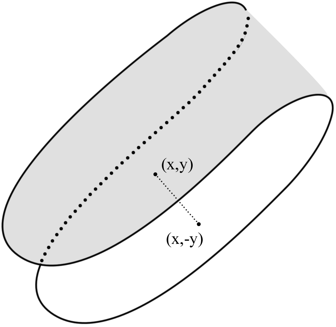
Figure 4.1: A section of the plate bent in half.

The heat equation which determines the temperature $u$ on the plate for this situation is given by

$$\frac{\partial{u}}{\partial t}(t,x,y)=\alpha\left[\frac{\partial^{2}u}{\partial x^{2}}(t,x,y)+\frac{\partial^{2}u}{\partial y^{2}}(t,x,y)\right]+\beta[u(t,x,-y)-u(t,x,y)],$$

where

$$\frac{\partial{u}}{\partial t}(t,x,y)=\alpha\left[\frac{\partial^{2}u}{\partial x^{2}}(t,x,y)+\frac{\partial^{2}u}{\partial y^{2}}(t,x,y)\right],$$

is the usual heat equation with heat transfer coefficient $\alpha>0$ and the term that goes with $\beta>0$ relates to the heat transfer from the corollaryresponding point in the other half of the plate due to Newton’s law of cooling.

If we consider the associated stationary problem

$$\alpha\left[\frac{\partial^{2}u}{\partial x^{2}}(x,y)+\frac{\partial^{2}u}{\partial y^{2}}(x,y)\right]+\beta[u(x,-y)-u(x,y)]=0,$$

it can be rewritten in a convenient way as

$$Lu:=\alpha\Delta u+\beta(A^{*}-\operatorname{Id})u=0,$$

where

$$\Delta=\frac{\partial^{2}}{\partial x^{2}}+\frac{\partial^{2}}{\partial y^{2}}\text{ and }A=\begin{pmatrix}1&0\\ 0&-1\end{pmatrix}.$$

If we think of a circular plate in which the boundary is constantly cooled and the surface has a constant heat source given by a function $h$, we are imposing Dirichlet boundary conditions in the ball $B$ of radius $\rho\in{\mathbb R}^{+}$ and considering the problem

$$Lu=h,\ u|_{\partial B}=0.$$ (4.3)

Observe that, $\Delta$, expressed in tensor notation, is $\Delta=D_{\omega^{0}_{2}}$ where

$$\omega^{0}_{2}=\frac{1}{2}\left[(1,1)\odot(1,1)+(1,-1)\odot(1,-1)\right].$$

Besides, $A\omega^{0}_{2}=\omega^{0}_{2}$ and, thus, $\Delta A^{*}=A^{*}\Delta$. Hence, using Theorem 3.3, we have to take $R=-\alpha\Delta+\beta A^{*}+\beta\operatorname{Id}$ and thus

$$RL= -\alpha^{2}\Delta^{2}-\alpha\beta A^{*}\Delta+\alpha\beta\Delta+\alpha\beta A^{*}\Delta+\beta^{2}\operatorname{Id}-\beta^{2}A^{*}+\alpha\beta\Delta+\beta^{2}A^{*}-\beta^{2}\operatorname{Id}$$

$$= -\alpha^{2}\Delta^{2}+2\alpha\beta\Delta=(-\alpha^{2}\Delta+2\alpha\beta\operatorname{Id})\Delta.$$

Now, the boundary conditions transformed by $R$ are

$$0=Ru=-\alpha\Delta u+\beta A^{*}u+\beta u=-\alpha\Delta u,$$

that is, the reduced problem becomes

$$RLu=Rh=:f,\ u|_{\partial B}=0,\ \Delta u|_{\partial B}=0,$$ (4.4)

which is equivalent to the sequence of problems

$$\Delta u= v,\ u|_{\partial B}=0,$$ (4.5)

$$(-\alpha^{2}\Delta+2\alpha\beta\operatorname{Id})v= f,\ v|_{\partial B}=0.$$ (4.6)

Problem (4.5) is the well-known Poisson equation with Dirichlet conditions on the circle of radius $\rho$. The Green’s function can be written in polar coordinates as

$$G_{1}(r,\varphi,\tilde{r},\tilde{\varphi})=\frac{-1}{4\pi}\ln\left[\frac{r^{2}\tilde{r}^{2}-2\rho^{2}r\tilde{r}\cos(\varphi-\tilde{\varphi})+\rho^{4}}{\rho^{2}r^{2}-2\rho^{2}r\tilde{r}\cos(\varphi-\tilde{\varphi})+\rho^{2}\tilde{r}^{2}}\right].$$

See [9, Section 7.2.3]. On the other hand, problem (4.6) is a Helmholtz equation, and the Green’s function can be described in terms of the eigenfunctions of the associated homogeneous problem (see [9, Section 7.3.3]). More concretely, the associated Green’s function in polar coordinates is written as

$$G_{2}(r,\varphi,\tilde{r},\tilde{\varphi})$$

$$= \frac{1}{\alpha^{2}}\sum_{n=0}^{\infty}\sum_{m=1}^{\infty}\frac{1}{\left(\frac{\mu_{nm}^{2}}{\rho^{2}}+\frac{2\beta}{\alpha}\right)\|w_{nm}^{(1)}\|^{2}}\left[w_{nm}^{(1)}(r,\varphi)w_{nm}^{(1)}(\tilde{r},\tilde{\varphi})+w_{nm}^{(2)}(r,\varphi)w_{nm}^{(2)}(\tilde{r},\tilde{\varphi})\right],$$

where $\mu_{nm}$ are the positive zeroes of the Bessel functions $J_{n}$, the eigenfunctions are given by

$$w_{nm}^{(1)}=J_{n}\left(\frac{\mu_{nm}}{\rho}r\right)\cos n\varphi,\quad w_{nm}^{(2)}=J_{n}\left(\frac{\mu_{nm}}{\rho}r\right)\sin n\varphi,$$

and

$$\|w_{nm}^{(1)}\|^{2}=\frac{1}{2}\pi\rho^{2}(1+\delta_{n\,0})\left[J_{n}^{\prime}(\mu_{nm})\right]^{2},$$

where $\delta_{ij}=1$ if $i=j$ and $0$ if $i\neq j$.

Now, the Green’s function associated to problem (4.4) is given by

$$G_{3}(r,\varphi,\tilde{r},\tilde{\varphi})=\int_{0}^{\rho}\int_{0}^{2\pi}G_{2}(r,\varphi,\hat{r},\hat{\varphi})G_{1}(\hat{r},\hat{\varphi},\tilde{r},\tilde{\varphi})\operatorname{d}\hat{\varphi}\operatorname{d}\hat{r}.$$

In conclusion, the Green’s function related to problem (4.3) is

$$G_{4}(\eta,\xi)=R_{\vdash}G_{3}(\eta,\xi)=\int_{0}^{\rho}\int_{0}^{2\pi}R_{\vdash}G_{2}(r,\varphi,\hat{r},\hat{\varphi})G_{1}(\hat{r},\hat{\varphi},\tilde{r},\tilde{\varphi})\operatorname{d}\hat{\varphi}\operatorname{d}\hat{r},$$

where $R_{\vdash}$ has to be expressed in polar coordinates in order to act in the first two variables of $G_{3}$:

$$R=-\alpha\left[\frac{\partial^{2}}{\partial r^{2}}+\frac{1}{r}\frac{\partial}{\partial r}+\frac{1}{r^{2}}\frac{\partial^{2}}{\partial\varphi^{2}}\right]+\beta A^{*}+\beta\operatorname{Id}.$$

Also, it is known that $J_{n}^{\prime}(z)=(n/z)J_{n}(z)-J_{n+1}(z)$, so

$$R_{\vdash}G_{2}(r,\varphi,\hat{r},\hat{\varphi})$$

$$= \frac{1}{\alpha^{2}}\sum_{n=0}^{\infty}\sum_{m=1}^{\infty}\frac{1}{\left(\frac{\mu_{nm}^{2}}{\rho^{2}}+\frac{2\beta}{\alpha}\right)\|w_{nm}^{(1)}\|^{2}}\left[\tilde{w}_{nm}^{(1)}(r,\varphi)w_{nm}^{(1)}(\tilde{r},\tilde{\varphi})+\tilde{w}_{nm}^{(2)}(r,\varphi)w_{nm}^{(2)}(\tilde{r},\tilde{\varphi})\right],$$

where

$$\tilde{w}_{nm}^{(1)}= \left.\left(\left(\frac{\mu_{nm}}{\rho}\right)^{2}\left[\left(\frac{n\rho}{\mu_{nm}r}\right)^{2}J_{n}-\left(1+\frac{(n+1)\rho}{\mu_{nm}r}\right)J_{n+1}+J_{n+2}\right]\right.\right.$$

$$\left.\left.+\frac{n}{r}\left[\frac{\rho}{\mu_{nm}r}J_{n}-J_{n+1}\right]-n^{2}\left(\frac{\mu_{nm}}{\rho}r\right)^{-2}J_{n}\right)\right|_{\left(\frac{\mu_{nm}}{\rho}r\right)}\cos n\varphi,$$

$$\tilde{w}_{nm}^{(2)}= \left.\left(\left(\frac{\mu_{nm}}{\rho}\right)^{2}\left[\left(\frac{n\rho}{\mu_{nm}r}\right)^{2}J_{n}-\left(1+\frac{(n+1)\rho}{\mu_{nm}r}\right)J_{n+1}+J_{n+2}\right]\right.\right.$$

$$\left.\left.+\frac{n}{r}\left[\frac{\rho}{\mu_{nm}r}J_{n}-J_{n+1}\right]-n^{2}\left(\frac{\mu_{nm}}{\rho}r\right)^{-2}J_{n}\right)\right|_{\left(\frac{\mu_{nm}}{\rho}r\right)}\sin n\varphi.$$

exa 4.2.

Inspired by the previous problem, we now change the term due to Newton’s law of cooling by a diffusion term in the following way.

$$\frac{\partial{K}}{\partial t}(t,x,y)=\alpha\left[\frac{\partial^{2}K}{\partial x^{2}}(t,x,y)+\frac{\partial^{2}K}{\partial y^{2}}(t,x,y)\right]+\beta\left[\frac{\partial^{2}K}{\partial x^{2}}(t,x,-y)+\frac{\partial^{2}K}{\partial y^{2}}(t,x,-y)\right],$$

where $\alpha,\beta>0$, $\beta\neq\alpha$.

If we consider the associated stationary problem

$$\alpha\left[\frac{\partial^{2}K}{\partial x^{2}}(x,y)+\frac{\partial^{2}K}{\partial y^{2}}(x,y)\right]+\beta\left[\frac{\partial^{2}K}{\partial x^{2}}(x,-y)+\frac{\partial^{2}K}{\partial y^{2}}(x,-y)\right]=0,$$

it can be rewritten as

$$LK:=\alpha\Delta K+\beta A^{*}\Delta K=0,$$

Using Theorem 3.3, we take $R=-\alpha\Delta+\beta A^{*}\Delta$ and then

$$RL=-\alpha^{2}\Delta^{2}-\alpha\beta\Delta A^{*}\Delta+\beta\alpha A^{*}\Delta^{2}+\beta^{2}(A^{*}\Delta)^{2}=\beta^{2}\Delta^{2}-\alpha^{2}\Delta^{2}=(\beta^{2}-\alpha^{2})\Delta^{2}.$$

Now, if we consider the fundamental solution of the bi-Laplacian $\Delta^{2}$ [6, equation (2.61)] we obtain a Green’s function given by

$$G_{1}(\eta,\xi)=\frac{1}{8\pi}\|\eta-\xi\|^{2}\ln\|\eta-\xi\|,\ \eta,\xi\in{\mathbb R}^{2}.$$

Hence, in that case, the Green’s function associated to $L$ is given by

$$G_{2}(\eta,\xi)=R_{\vdash}G_{1}(\eta,\xi)=(\beta-\alpha)\frac{\ln\|\eta-\xi\|+1}{2\pi},\ \eta,\xi\in{\mathbb R}^{2}.$$

If we consider the problem

$$LK=h,\ u|_{\partial B}=0,$$

the reduced problem becomes

$$(\beta^{2}-\alpha^{2})\Delta^{2}K=h,\ u|_{\partial B}=0,\ Ru|_{\partial B}=0.$$ (4.7)

Now, the condition $Ru=-\alpha\Delta u+\beta A^{*}\Delta u=0$ is satisfied if we can guarantee that $\Delta u=0$, so we can consider the problem

$$(\beta^{2}-\alpha^{2})\Delta^{2}K=h,\ u|_{\partial B}=0,\ \Delta u|_{\partial B}=0.$$ (4.8)

For problem (4.8) we have that the Green’s function is given by

$$G_{3}(\eta,\xi)=\frac{1}{8\pi}\|\eta-\xi\|^{2}\left(\ln\rho-1+\ln\|\eta-\xi\|\right)+\frac{\rho^{2}}{8\pi},\ \eta,\xi\in{\mathbb R}^{2}.$$

Hence, the Green’s function related to problem (4.7) is

$$G_{4}(\eta,\xi)=\frac{\ln\rho+\ln\|\eta-\xi\|}{2\pi}.$$

In general, the functions

$$G_{5}(\eta,\xi)=\frac{1}{8\pi}\|\eta-\xi\|^{2}\left(\mu+\ln\|\eta-\xi\|\right)+\frac{\nu}{8\pi},\ \eta,\xi\in{\mathbb R}^{2},$$

with $\mu,\,\nu\in{\mathbb R}$, are Green’s functions related to the operator $\Delta^{2}$ with different boundary conditions. The associated function for the operator $L$ is given by

$$G_{6}(\eta,\xi)=\frac{1+\mu+\log\|\eta-\xi\|}{2\pi}.$$

References

• [1] Amir-Moéz, A.R., Palmer, D.W.: Characterization of linear involutions. Univ. Beograd. Publ. Elektrotehn. Fak. Ser. Mat. 4, 23–24 (1993)
• [2] Burlutskaya, M.S., Khromov, A.: Initial-boundary value problems for first-order hyperbolic equations with involution. Dokl. Math. 84(3), 783–786 (2011)
• [3] Cabada, A., Tojo, F.A.F.: Comparison results for first order linear operators with reflection and periodic boundary value conditions. Nonlinear Anal. 78, 32–46 (2013)
• [4] Cabada, A., Tojo, F.A.F.: Green’s functions for reducible functional differential equations. Bull. Malays. Math. Sci. Soc. (2016)
• [5] Fock, V.: Konfigurationsraum und zweite Quantelung. Zeitschrift für Physik 75(9-10), 622–647 (1932)
• [6] Gazzola, F., Grunau, H.C., Sweers, G.: Polyharmonic boundary value problems: positivity preserving and nonlinear higher order elliptic equations in bounded domains. 1991. Springer Science & Business Media (2010)
• [7] Helton, J.W., de Oliveira, M., Stankus, M., Miller, R.L.: NCAlgebra - Version 4.0.6 (2015). URL http://math.ucsd.edu/~ncalg/
• [8] Kirane, M., Al-Salti, N.: Inverse problems for a nonlocal wave equation with an involution perturbation. JOURNAL OF NONLINEAR SCIENCES AND APPLICATIONS 9(3), 1243–1251 (2016)
• [9] Polyanin, A.: Handbook of linear partial differential equations for engineers and scientists. CRC Press Company (2002)
• [10] Silberstein, L.: Solution of the equation $f(x)=f(1/x)$. Lond. Edinb. Dubl. Phil. Mag. 30(200), 185–186 (1940)
• [11] Wiener, J.: Generalized solutions of functional differential equations. World Scientific (1993)