Memory vs. irreversibility in thermal densification of amorphous glasses

Abstract

We report on dynamic effects associated with thermally-annealing amorphous indium-oxide films. In this process the resistance of a given sample may decrease by several orders of magnitude at room-temperatures, while its amorphous structure is preserved. The main effect of the process is densification - increased system density. The study includes the evolution of the system resistivity during and after the thermal-treatment, the changes in the conductance-noise, and accompanying changes in the optical properties. The sample resistance is used to monitor the system dynamics during the annealing period as well as the relaxation that ensues after its termination. These reveal slow processes that fit well a stretched-exponential law, a behavior that is commonly observed in structural glasses. There is an intriguing similarity between these effects and those obtained in high-pressure densification experiments. Both protocols exhibit the ”slow spring-back” effect, a familiar response of memory-foams. A heuristic picture based on a modified Lennard-Jones potential for the effective interparticle interaction is argued to qualitatively account for these densification-rarefaction phenomena in amorphous materials whether affected by thermal-treatment or by application of high-pressure.

.1 Introduction

The mass-density of a solid is one of its most characteristic features. In crystalline materials the density hardly changes even under the application of large pressures. Yet, even a minor volume difference may induce a conspicuous and sometime dramatic change of a measured property of the material. Structural glasses, on the other hand, often show considerable volume change $\Delta$V under pressure; relative volume shrinkage $\Delta$V/V exceeding 15% was observed in a number of studies 1 ; 2 ; 3 ; 4 ; 5 ; 6 ; 7 ; 8 ; 9 ; 10 ; 11 ; 12 ; 13 . Glasses are often amorphous structures, namely solids that lack long-range spatial order, and it is this group of glasses that is addressed in this paper.

The increase in density under pressure was originally thought to be an irreversible, permanent phenomenon 2 . Later studies revealed hysteretic effects in the pressure dependence of electronic 6 and optical 1 properties of glasses. The observed hysteresis during a pressure cycle was partly associated with artifacts inherent in the technique 6 but there were also indications for slow recovery from the densified phase when the pressure was relieved in optical studies 7 . These perhaps gave the impression that a rarefied state may be the more energetically favored of the amorphous solid.

Densification of amorphous solids by pressure is intuitively expected. It is less trivial that volume shrinkage could also be affected by thermal-annealing. For example, subjecting amorphous indium-oxide (In${}_{\text{x}}$O) films to a series of thermal-treatments at temperature that exceeded the temperature T${}_{\text{P}}$ at which they were prepared, resulted in density increase by 3-20%, depending on their composition 14 . The reduced density was reflected in the optical properties as a downward shift of the optical-gap and concomitant increase of the refractive index while their amorphous structure remained essentially intact 14 . The relative magnitude of these changes was comparable to the respective changes observed in high-pressure densification experiments 1 ; 2 .

During densification, by either pressure or thermal-annealing, the room-temperature resistivity of amorphous films may change by several orders of magnitude 6 . In the In${}_{\text{x}}$O system a change in resistivity of five-six orders of magnitude was shown to be related to the volume shrinkage while the carrier-concentration was affected by less than a factor of three 15 . This technique has been used to study the metal-insulator and the superconductor-insulator transitions in In${}_{\text{x}}$O with various In-O compositions 16 as well as to assess the magnitude of disorder in the insulating phase 14 .

The present study started as a follow-up on the latter issue by measuring the changes in the 1/f-noise as function of disorder that is presumably modified during the annealing process. As will be shown in section III, the magnitude of the flicker-noise does indeed change systematically with the resistivity of the system. However, there appeared to be large fluctuations in the data that led us to find, as a possible reason, a non-stationary state of the system that follows the thermal-annealing protocol. The current work is dedicated to the elucidation of this state an in particular to gain insight to its dynamics.

The sensitivity of the system conductivity to even a small structural change is utilized in this work to continuously monitor the densification process during thermal-annealing, as well as during the system relaxation that takes place after the heating power is turned off and the sample regains its (quasi)-equilibrium temperature. A series of in-situ experiments performed in this study establishes a correlation between the change in the system resistivity and its optical transmission. This allows us to compare our results with other glasses where only optical properties were measured, and draw conclusions that may be pertinent to general aspects of densification-rarefaction phenomena. A heuristic picture is presented that offers a plausible explanation for the out of equilibrium effects that accompany these phenomena in amorphous glasses whether driven by thermal-treatment or application of pressure.

.2 Samples preparation and characterization

The In${}_{\text{x}}$O films used here were e-gun evaporated on room-temperature substrates using 99.999% pure In${}_{\text{2}}$O${}_{\text{3}}$ sputtering target pieces. Two types of substrates were used; glass microscope-slides 1mm thick for electrical measurements, and quartz float-glass 2 mm thick for the in-situ optics+resistance measurements. Deposition was carried out at the ambience of (2-5)·10${}^{\text{-4}}$ Torr oxygen pressure maintained by leaking 99.9% pure O${}_{\text{2}}$ through a needle valve into the vacuum chamber (base pressure $\simeq$10${}^{\text{-6}}$ Torr). Rates of deposition were 0.3-0.6 Å/s. For this range of rate-to-oxygen-pressure, the In${}_{\text{x}}$O samples had carrier-concentration N in the range (8-12)·10${}^{\text{19}}$cm${}^{\text{-1}}$ measured by Hall-Effect at room temperature. The films thickness in this study was 400-1000 Å. Lateral sizes varied from 0.2x0.2mm${}^{\text{2}}$ (for the 1/f noise studies), 1x1mm${}^{\text{2}}$ for the thermal-annealing in the small vacuum cell, and 2x2cm${}^{\text{2}}$ for the in-situ optics-resistance vacuum-cell. The evaporation source to substrate distance in the deposition chamber was 45cm. This yielded films with thickness uniformity of $\pm$2% across a 2x2cm${}^{\text{2}}$ area.

The as-deposited samples typically had sheet-resistance R_□ of the order of $\approx$5·10${}^{\text{7}}\Omega$ for a film thickness of $\approx$10${}^{\text{3}}$Å. This was usually the starting stage for the thermal-annealing protocols performed on each preparation batch (14 different batches were used in the study). A comprehensive description of the annealing process and the ensuing changes in the material microstructure are described elsewhere 15 ; 16 .

Each deposition batch included samples for optical excitation measurements, samples for Hall-effect measurements, and samples for structural and chemical analysis using a transmission electron microscope (TEM). For the latter study, carbon-coated Cu grids were put close to the sample during its deposition and received the same post-treatment as the samples used for transport measurements. TEM work was only performed on two of the preparation batches used here, mainly to check on the integrity of the procedure by comparing with our past studies of In${}_{\text{x}}$O films 14 ; 15 ; 16 .

.3 Measurement techniques

Following removal from the deposition chamber, the sample was mounted onto a heat-stage in a small vacuum cell equipped with contacts for electrical measurements and a thermocouple thermometer. Two cells were employed in our study. The first (cell #1) was used for the noise and resistance measurements and had a light-weight heating-stage made of 0.2mm strip of copper. This allowed for quicker changes of temperature than the one used for optics being made of heavier 0.5mm copper sheet (cell #2). The characteristic time to reach 90% of the asymptotic temperature after applying power to the heating-stage was typically $\approx$300s for the cell #1 and $\approx$700s for cell #2 used for optics measurements. Cell #2 was installed in the measuring compartment of the Cary-1 spectrophotometer. In addition to electrical wires fed trough this cell for resistance and temperature measurements it featured two quartz windows that allowed in-situ transmission measurements during several stages of annealing protocols. Each optical-transmission measurement was preceded by taking a transmission scan over the wavelength range of $\lambda$=320-860nm using a blank substrate installed in a similar cell as that used for the actual sample. This scan was used as a baseline to eliminate the contribution of reflections associated with the five glass-air interfaces in the measurement set-up.

Copper wires were soldered to pressed-indium contacts to facilitate resistance measurements. These were performed by a two-terminal technique using either the computer-controlled HP34410A multimeter or the Keithley K617. Noise measurements employed PAR 5113 pre-amplifier and Agilient 35670A spectrum analyzer. The set-up involved measuring the voltage across a low-noise resistor in series with the sample and a variable-voltage battery.

I Results and discussion

I.1 Evolution of the resistance during a thermal-annealing protocol

The protocol we routinely use for thermal-annealing In${}_{\text{x}}$O samples is composed of the following steps: The sample, prepared at T${}_{\text{P}}$ (typically$\simeq$295$\pm$2K unless otherwise specified) is anchored to a heat-stage within the measuring cell that is then evacuated by a rotary-pump to a pressure of $\lesssim$0.03mbar). Next the heating stage is energized, and within a time interval $\delta$t it reaches an annealing temperature T${}_{\text{A}}$. The system is then kept at this temperature for a dwell-time t${}_{\text{d}}$, typically much longer than $\delta$t. Finally, the heat supply is turned off and the sample is cooled back to ambient temperature within essentially the same $\delta$t as in the heat-up stage. Figure 1 illustrates a detailed R(t) behavior for such protocol. For brevity, the notation $\Delta$T$\equiv$T${}_{\text{A}}$-T${}_{\text{P}}$ is used in all figures depicting thermal-annealing protocols.

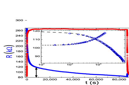
Figure 1: A typical protocol used in thermal-annealing of In${}_{\text{x}}$O films. Resistance data R(t) are shown in circles and refer to the left scale, the sample temperature above room’s $\Delta$T(t)$\equiv$T${}_{\text{A}}$(t)-T${}_{\text{P}}$ is plotted with squares and refer to the right scale. The sample here has a thickness of 50nm and lateral dimension of 1x1mm${}^{\text{2}}$. The arrows mark the onset of constant-temperature time-intervals starting from which fits are shown (dashed lines) to R(t) associated with the annealing process (8,000s$<$t$<$86,000s) and relaxation (t$>$92,000s). The fits to the data in the inset (circles for annealing, triangles for relaxation), are based on Eq.1 and Eq.2. These use the parameters $\beta$=0.6, 0.5 and $\tau$=390,000s, 8,000s respectively. To accommodate both curves in the inset, the data and fit for the relaxation part are shifted by a constant while the origin of the time scale is the position of the respective arrow.

120

Note first the relatively sharp response of the resistance over $\delta$t when heating is applied and the temperature is approaching T${}_{\text{A}}$, and the similarly fast change of R during the cooling-back to T${}_{\text{P}}$. These sharp responses are mostly due to the temperature dependence of the sample resistivity. The temperature coefficient of the resistance (TCR), for most of the samples reported here, is negative (a sample with a positive TCR will be shown in Fig.6 below for comparison). The focus in this work however is on the processes that occur while the temperature is constant, either during the heating-period (under T${}_{\text{A}}$) or after the system temperature is back at T${}_{\text{P}}$. During these time-intervals the system resistance R evolves with time in a systematic manner:

Under T${}_{\text{A}}$, the resistance decreases monotonically and $\Delta$R(T) follows a stretched-exponential time dependence:

$$\Delta\text{R(t)}=\text{R}_{\text{0}}\exp\text{[-(t/}\tau\text{)}^{\beta}\text{]}$$ (1)

Once the system settles back at T${}_{\text{P}}$, the resistance slowly climbs back up, also with a stretched-exponential law:

$$\Delta\text{R(t)}=\delta\text{R}_{\text{a}}\text{\{1-}\exp\text{[-(t/}\tau\text{)}^{\beta}\text{]\}}$$ (2)

These functional dependences seem to be reasonably good fits to the data over both time intervals where the sample temperature is constant if the exponent $\beta$ is $\approx$0.5-0.6 (Fig.1). In fact, all our data for R(t) in the relaxation regime of the annealing-cycle can be fitted to Eq.2 with $\beta$=0.5.

Stretched-exponential time dependence, with $\beta\approx$ 0.5-0.6, is commonly observed in the dynamics of structural glasses 17 ; 18 . Several scenarios for the origin of the stretched-exponential dependence and it physical meaning were discussed in the literature 19 . A simple interpretation that is sometimes used suggests that the stretched-exponential is just a weighted sum of simple exponentials reflecting an underlying heterogeneity of the system 20 ; The relaxation function is the convoluted effect of parallel relaxation events with distributed relaxation times. It this picture the parameter $\beta$ is a logarithmic measure of the distribution width and $\tau$ is a characteristic relaxation time 20 .

Fitting data of a rather simple form such as our R(t) plots to Eq.1 or Eq.2, involving 3 parameters is not critical enough to distinguish between possible scenarios. These fits will be used in this work only to get an estimate for the asymptotic value of the resistance and as rough tool to get a typical value of the relaxation-time $\tau$ involved in the dynamics. We note in passing that, in contrast to the electron-glass dynamics 21 , these R(t) data cannot be fitted to a logarithmic-law neither during the annealing period nor during the relaxation that takes place after the system temperature is reset to and stabilizes at T${}_{\text{P}}$; even on half a decade in time one observes conspicuous deviations from a log(t) dependence (see e.g., inset to Fig.1).

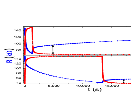
Figure 2: Thermal-annealing protocol for two samples using different heating-periods. Samples are from the same batch with a thickness of 50nm. They were subjected to a similar temperature during annealing; T${}_{\text{A}}$=357$\pm$1K, and T${}_{\text{A}}$=355$\pm$1K for (a) and (b) respectively. The arrows indicate the points at which T${}_{\text{P}}$ has reached constant temperature.

There appears to be a threshold temperature increment $\Delta$T^′ for getting densification, which may be (somewhat arbitrarily) defined as the minimum temperature increment under which a systematic reduction of the resistance is observed during the thermal-treatment. Empirically, $\Delta$T^′ depends on the specific preparation batch and on sample history. In as-prepared samples studied here $\Delta$T^′ varied between $\approx$5K to $\approx$20K. When the applied $\Delta$T was smaller than $\Delta$T^′ the resistance during the heating-period may not have changed at all even when the heating was kept for 24 hours. In one instance a sample with R$\approx$60M$\Omega$ was kept under $\Delta$T=11K for three weeks while R was just fluctuating around the resistance value it had at T${}_{\text{A}}$ with no sign of irreversible change.

The reduction of the sample resistance during the heating-period has been used to change the sample resistance in studies of the metal-insulator and superconducting-insulator transitions (MIT and SIT respectively 16 ). By a judicious choice of $\Delta$T and the time of annealing one can fine-tune the disorder and scan the immediate vicinity of the MIT (or SIT) working with a single physical sample making this procedure an efficient technique for these studies.

The MIT and SIT experiments naturally involve low-temperatures where the dynamics associated with the resistance creep-up was effectively frozen. For this reason not much attention has been given to the recovery of resistance once the process is terminated and $\Delta$T is set back to zero. When noticed, the slow recovery of resistance that ensued after thermal-annealing was terminated has been ascribed to a quench-cooling effect counteracting the annealing process. Unfortunately, it is not easy to test this conjecture experimentally; to eliminate this effect one may need to cool the sample back to T${}_{\text{P}}$ at a much lower rate than the typical relaxation rate of the system, which besides being time consuming is susceptible to being tainted by accidental artifacts.

On the other hand it can be demonstrated that, all other things being equal, the relative amount of the resistance that is asymptotically recovered depends in a systematic way on the time the system spends under a given T${}_{\text{A}}$.

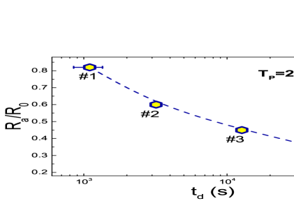
Figure 3: The ratio between the resistance before and after thermal-annealing as function of the dwell-time t${}_{\text{d}}$ the sample was under a temperature of T${}_{\text{A}}$=356$\pm$2K. Data points stand for four different samples from the same preparation batch (50nm thick). Sample #1 and #3 are the same samples shown in Fig.2 (a) and Fig.2 (b) respectively.

An example for the role of time is shown in Fig.2: The data in the figure illustrates that, other things being equal, shorter dwell-time results in a larger magnitude of recovered resistance (Fig.2a). The R(T) for the final stage of the protocol, fitted to the stretched-exponential law (yielding similar values for $\beta$=0.5 and $\tau\approx$10${}^{\text{4}}$) was used to estimate the asymptotic values R${}_{\text{a}}$=R(t$\rightarrow\infty$) for both Fig.2a and Fig.2b data. From these one infers that thermal-annealing has reduced the resistance by $\approx$20% for the sample in Fig.2a and by $\approx$120% for the sample in Fig.2b, while the dwell-times were $\approx$1100s and $\approx$13,000s respectively.

For a more detailed view of the role of time, one needs to quantify the change of the resistance caused by the thermal-treatment process. A quantitative measure of the annealing effect is the ratio R${}_{\text{0}}$/R${}_{\text{a}}$ between the initial resistance R${}_{\text{0}}$(T${}_{\text{P}}$) and the asymptotic value for it R${}_{\text{a}}$(T${}_{\text{P}}$). For the latter we extrapolate R(t) for t$\rightarrow\infty$ using Eq.2. The R${}_{\text{0}}$/R${}_{\text{a}}$ ratio as function of the annealing time is shown in Fig.3 for several samples from the same preparation batch.

Once $\Delta$T$>$$\Delta$T^′, such that some degree of densification is affected, a finite magnitude of resistance is recovered at the asymptotic regime even when the drop of the initial resistance during the thermal-annealing is very large as is the case in Fig.4.

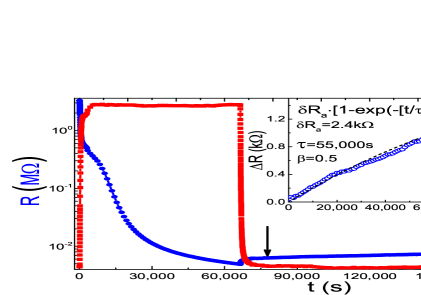
Figure 4: Thermal-annealing protocol (notations as in Fig.1) for a sample with a thickness 96nm. Note the log scale for the R(t) data to expose the small recovered-resistance component that follows the termination of the heating-period. The inset shows a fit to the relaxation using Eq.2 with the parameters shown in the inset (origin for the time and for $\Delta$R are marked by the arrow).

On the other extreme, a short dwelling-time, results in most of the original resistance being recovered as depicted in Fig.5.

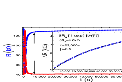
Figure 5: Thermal-annealing protocol for a sample with thickness of 100nm. The sample has been under T${}_{\text{A}}$ =287$\pm$2K for $\approx$250s. Its initial resistance R${}_{\text{0}}$ was 134k$\Omega$ and its asymptotic resistance R${}_{\text{a}}$ (extrapolated through the fit to Eq.2 see inset) is 133k$\Omega$. All notations are as in Fig.4.

All examples for thermal-annealing shown above involve samples that are on the insulating side of the MIT and, in particular, exhibit a negative TCR ($\partial$R/$\partial$T$<$0) over the temperature range of our experiments. This may raise the question of whether the slow recovery of the resistance is related to a sluggish cooling process of the electronic system. The results of the protocol shown in Fig.6 show that the R-recovery is independent of the TCR sign. In this case the process of thermal annealing was extended for a long time and under a relatively large $\Delta$T to reduce the system disorder to below the value where the TCR changes sign and becomes positive. Still, the recovered resistance at the end of the process has the same sign and temporal functional dependence as when $\partial$R/$\partial$T was negative.

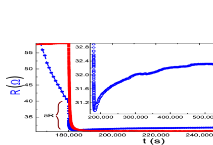
Figure 6: Thermal-annealing run on a sample with thickness of 100nm heated to 393K for 50 hours. This is the last heating cycle in an annealing series that started with the sample having R$\approx$10M$\Omega.$ The main graph shows the last 4 hours of heating and the drop of R upon terminating the heating (illustrating a positive TCR). The inset is an expanded view of the recovery process and shows R(t) monitored for almost 6 days at T=295$\pm$1K. During this process the sample resistance changed from $\approx$2k$\Omega$ to an asymptotic value of R= 32.3$\Omega$.

The behavior of the resistance during the annealing-protocol has a mechanical analogue; The thickness of a sponge subjected to the squashing effect of a heavy object will show qualitatively similar time-dependence as R(t) in the examples above. In particular, it will swell back towards its original thickness, initially as a rather fast jump followed by a much slower process. The thickness will asymptotically recover to a degree dependent on the time spent under the weight. In some sense, the sponge exhibits a memory of its pristine dimensions much like the tendency of the amorphous system to recover part of its resistance. In both cases the recovery is partial; recovery is limited by the irreversible changes that the system incurs during heat-treatment (or during the time the system is under pressure). These changes are responsible for what has been referred to as ”permanent” densification 1 ; 2 ; 3 ; 4 ; 5 ; 7 ; 8 ; 9 and will be discussed later.

It is implicitly assumed in this work that changes in resistance occurring while the temperature is fixed at T${}_{\text{A}}$, T${}_{\text{P}}$ reflect densification, rarefaction respectively. This notion is supported by measurements of the optical changes that take place during these processes.

I.2 Density changes probed by optics

The main structural change caused by thermally-annealing In${}_{\text{x}}$O films was shown to be increased mass-density by measuring the sample thickness before-and-after the heat-treatment using x-ray interferometry 14 . The decrease of the sample volume in the process was also reflected in a downward shift of the optical-gap and an increase of the refractive index 14 . These modified optical properties were correlated with the concomitant changes in the system resistance. This correlation however was established for the quasi-stationary situation, not during the time-intervals where the system is evolving towards higher or lower density. The data shown in Fig.7 and Fig.8 were taken to test the correlation between optics and resistance during these periods.

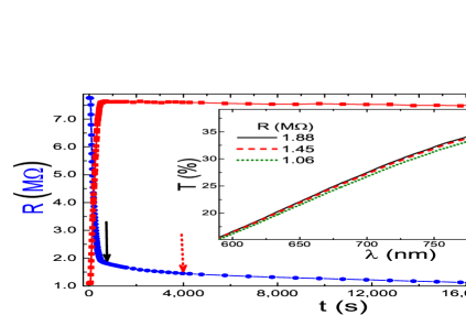
Figure 7: A 96nm thick In${}_{\text{x}}$O sample kept under a constant T${}_{\text{A}}$=347$\pm$1K for 5.5 hours. During this time R slowly decreased and optical transmission curves (inset) were taken at three different resistances at times marked by arrows that are coded to match the marked resistance-values.

In these experiments, optical transmission-traces were taken at several points in time while a constant T${}_{\text{A}}$ was maintained (Fig.7) and after the sample temperature was reset and stabilized at T${}_{\text{P}}$ (Fig.8). R(t) of the respective sample was continuously recorded during these time intervals. Figure 8 illustrates how transmission data (Fig.9a) may be used to obtain the shift in the optical-gap E${}_{\text{g}}$ (Fig.9b) which is indicative of a volume change; a downward shift in E${}_{\text{g}}$ means densification 14 . The data in Fig.8 were taken on the same preparation batch of In${}_{\text{x}}$O as the samples in Fig.7 and Fig.8. The $\approx$85mV reduction of the optical-gap and the $\approx$3 orders of magnitude resistance-decrease result from the enhanced overlap of the atomic wavefunctions during the thermal densification process 14 . This illustrates the higher sensitivity to volume change of the resistance measurement technique. In fact, the relative change of the sample resistance caused by thermal-annealing, is exponential with the corresponding change in the optical transmission 6 . This was confirmed here using the data for the samples shown in Figures 7,8 and 9 (all from the same In${}_{\text{x}}$O preparation batch).

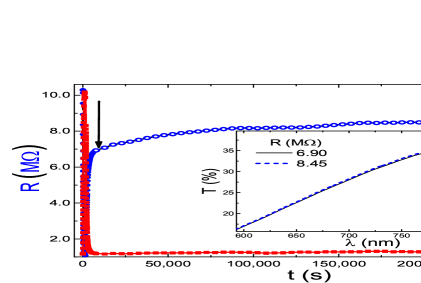
Figure 8: A 96nm thick In${}_{\text{x}}$O sample heated for $\approx$300s under T${}_{\text{A}}$=373K$\pm$1K then cooled to room-temperature and its R(t) was recorded for $\approx$68 hours. Optical transmission traces (shown in inset) were taken during the R-recovery process at times and resistance-values indicated by the arrows.

The temporal resolution of the resistance measurement is also far superior to the optics; Optical transmission measurement over the wavelength shown in Figures 7 and 8 typically took 200s to get a well-averaged signal while the time constant for the resistance measurement is $\approx$1s.

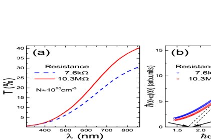
Figure 9: Optical transmission (a) and absorption (b) for a 96nm In${}_{\text{x}}$O sample (from the same batch as in Figs.7&8). Data taken at T=295K.

The optics measurements in Fig.7 suggest densification, consistent with the decrease of the sample resistance accumulated over the time the sample temperature was fixed at T${}_{\text{A}}$. Similarly, the transmission data in Fig.8 imply that during the time the sample relaxes after its temperature reaches T${}_{\text{P}}$, the system volume and its resistance slowly increase with time.

I.3 Comparison with pressure-induced densification

It is interesting to compare the effects due to thermally-annealing In${}_{\text{x}}$O films to those obtained on other glasses by applying high pressure. We have to restrict this comparison however to the quasi-static features of the phenomena as the details of the dynamics has yet to be systematically studied in high-pressure experiments (presumably due to inadequate temporal resolution inherent to the technique).

There is comprehensive literature on pressure-induced densification studies spread over almost seven decades and involving more than ten different materials 1 ; 2 ; 3 ; 4 ; 5 ; 6 ; 7 ; 8 ; 9 ; 10 ; 11 ; 12 ; 13 . In some experiments the change of volume was directly measured. In many studies however the property that was monitored was taken as indicatory of the volume decrease, which was taken for granted. In 6 , for example, the resistance of amorphous As${}_{\text{2}}$Te${}_{\text{3}}$ at room temperature was this property. It was observed to drop by 6-7 orders of magnitude with pressure of 100kBar. This is a similar swing of resistance obtained by thermal-annealing In${}_{\text{x}}$O samples, as in the series culminating in Fig.6 above. It only takes longer to get there by the thermal technique.

Indeed, it appears that the main difference between applying pressure and temperature is in the associated relaxation time. In terms of the qualitative features of the densification-rarefaction phenomena, the similarity between the two agents is remarkable. Let us review the main features of the phenomena as they appear when induced by the two techniques:

• As alluded to above, there seems to be a threshold $\Delta$T necessary for densification. A similar impression was formed already in early pressure works: ”A definite threshold pressure is observed in vitreous silica and silicate glasses, under which no effect takes place and above which the collapse takes place readily…” 1 , to give one example.

• There is a correlation between shrinkage of the system volume and a downward shift of the optical-gap in thermally-annealed In${}_{\text{x}}$O. The same correlation has been recognized in several high-pressure densification studies: ”…The red shift of optical absorption edge in the visible region that results from densification exhibited the same pressure dependence as that observed for density…” 12 .

• A common feature in all densification studies, independent of material and technique, is the asymptotic recovery of a material property that was changed from its original value during densification. This property may be the volume itself or, as in most cases, a property like optical-gap or resistance that reflects the volume change. Examples for this effect are abundant in this paper. This fact was frequently noticed in pressure studies as well: :…when pressure is relieved… it reverts to previous state…” 6 , ”…When the pressure is removed, the absorption edge shifts back to the high-energy side, but with hysteresis. After the pressure is removed, the absorption edge initially remains at a lower energy than the original value, but slowly increases…” 7 ,”…The densified state is found to be metastable and decreases in density over time spans of the order of years…” 8 .

The appearance of this rarefaction-effect in so many different glasses suggests an generic feature, characteristic of the glassy phase. In the following we examine a heuristic picture that may assist in understanding the observed phenomena and in particular, explains how thermal-annealing may induce densification as well as the reason for the difference in dynamics between applying high-pressure and subjecting the system to an elevated temperature.

I.4 A heuristic picture for densification-rarefaction

The picture we consider is based on the inter-particle potential schematically shown in Fig.10.

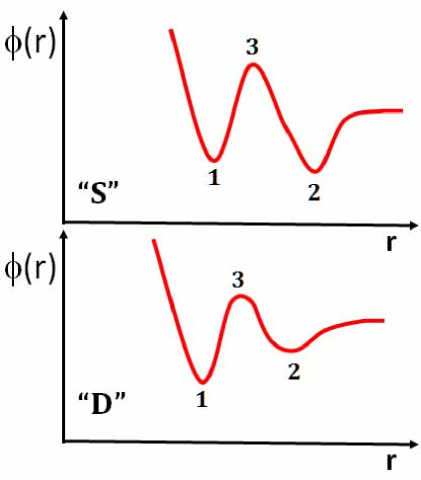
Figure 10: A schematic description of the effective interparticle-potential $\Phi$ versus their separation r. Two forms of this potential are shown as representatives from the assumed continuous distribution.

The figure depicts two local configurations of the interparticle potential; ”S” and ”D” are specific two-state-systems 22 ; 23 featuring two local minima. The state labeled S (for ”spongy”) favors a larger interparticle separation while D favors a dense structure. The system density at a given temperature and pressure is determined by the $\Phi_{i}$’s. Transitions of the type S,D(1$\rightarrow$2), S,D(2$\rightarrow$1), are assumed to be controlled by a Boltzmann factor:

$$\omega\text{\textperiodcentered exp[-}\delta\text{/k}_{\text{B}}\text{T]}$$ (3)

where $\delta$ is $\delta_{\text{3,1}}$=$\Phi$(3)-$\Phi$(1), $\delta_{\text{3,2}}$=$\Phi$(3)-$\Phi$(2) respectively, $\omega\approx$10${}^{\text{12}}$s${}^{\text{-1}}$ is the attempt-frequency and T is the temperature.

Many of the local configurations in the as-made In${}_{\text{x}}$O films, are probably ‘spongy’ because the samples were quench-condensed from the vapor phase onto room-temperature substrates and therefore are similar to rapidly-chilled glasses 1 . Accordingly, S-configurations may initially be preponderant in the system. When $\Delta$T$>$0 is applied the balance of occupation in the S(1) and S(2) states changes and the density will increase towards the level dictated by Boltzmann statistics and controlled by the distribution of the $\delta_{\text{3,2}}$ barriers. If, while $\Delta$T is on, there are no irreversible structural changes then the density will eventually saturate at the ‘equilibrium’ value set by the temperature. In this case the density will acquire its pristine value when $\Delta$T is reduced to zero. Memory is preserved in this case but full recovery of the resistance will be governed by the time the system spends under $\Delta$T and by the $\delta_{\text{3,1}}$-barriers.

The typical relaxation time associated with the resistance recovery may be estimated from the fitted value for $\tau$ in Eq.2. This parameter in our R(t)-recovery data (all measured at T${}_{\text{P}}$=295$\pm$2K), range between 7.7·10${}^{\text{3}}$s to 55·10${}^{\text{3}}$s. Using $\omega$·exp[-$\delta_{\text{3,1}}$/k${}_{\text{B}}$T] to estimate the associated typical barrier one gets $\delta_{\text{3,1}}\approx$1.1$\pm$0.05 eV, which is quite a reasonable value.

The situation where memory is perfect may only be realized when $\Delta$T is very small or when applied for a very short time. Occupation of S(1)-states for any length of time would change the interparticle interactions and some reconstruction may locally occur. Those regions where the reconstructions lowers the energy will sustain a modified form of the effective interparticle-potential.

Permanent densification hinges on converting S’s into D’s thus increasing the weight of dense configurations in the interparticle-potential distribution. Such a process involves reconstruction, which means that a number of atoms (of the order of the coordination number), have to change their position. The probability for this ‘many-body’ process to occur while the S(1) state is occupied, might also be represented by an effective barrier. The typical barrier $\delta_{\text{D}}$ for densification may then be estimated using for example the R(t) data from Fig.1; During densification R(t) was monitored for 87,000s under a constant T${}_{\text{A}}$=340$\pm$2K. These data fitted to Eq.1 with $\tau\approx$3.9·10${}^{\text{5}}$s (inset to Fig.1) gives $\delta_{\text{D}}$=1.5$\pm$0.1eV, somewhat larger than the typical barrier for relaxation.

Essentially the same scenario is expected for application of pressure. The main difference between raising the temperature or applying pressure is in the dynamics of the processes; Applying pressure reduces barriers for densification and may actually eliminate them completely 11 . This would swiftly collapse the system into the S(1) state. However, if pressure is relieved before local reconstruction occurs, slow rarefaction should be observed just as in the case of the $\Delta$T scenario. This slow recovery has indeed been observed in a number of high-pressure studies 8 ; 9 ; 13 .

Pressure is a more efficient way to achieve permanent densification as it may be large enough to suppress $\delta_{\text{3,2}}$, and even a small shear component (that often accompanies pressure application) is effective in locking-in irreversible changes 3 . Temperature is less effective in this regard as there is a limit to the $\Delta$T that one may apply without causing crystallization. For In${}_{\text{x}}$O the temperature should not exceed $\approx$450K 15 ; 24 , still much smaller than the typical barrier involved in densification $\delta_{\text{D}}$.

Densification by thermal-annealing has many advantages over pressure, especially for vapor deposited glasses such as the current system. It is not an efficient method for glasses that were obtained from the melt; these systems were subjected to T${}_{\text{A}}$ extending up to the glass temperature so they were already thermally-annealed to a certain degree. The history associated with the cooldown from the melt would play a role in future annealing protocols. Examples of protocols where history has a marked effect on relaxation are illustrated in Figs.11, and 12:

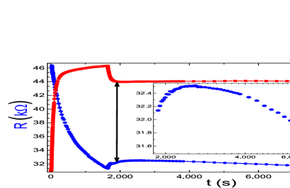
Figure 11: A two-temperatures annealing protocol. The sample, 50nm thick, is heated to and maintained at T${}_{\text{A}}$=348$\pm$2K for 1300s. Then, the temperature is changed and held at T${}_{\text{A}}$=340$\pm$1K. The resistance versus time recorded throughout the protocol exhibits a non-monotonic behavior (shows on an expanded scale in the inset) at the later stage of the protocol.

These figures show R(t) for a protocol with two annealing periods at different temperatures: after the system spends time under T${}_{\text{A}}$ the temperature is reduced and kept at intermediate temperature T${}_{\text{I}}\,$, T${}_{\text{P}}$$<$T${}_{\text{I}}$$<$ T${}_{\text{A}}$. Such a protocol is an attempt to thermally-anneal a system at T${}_{\text{I}}$$>$T${}_{\text{P}}$ after it was thermally-annealed at T${}_{\text{A}}$$>$T${}_{\text{I}}$ for a finite time t${}_{\text{d}}\lll\tau$. On the basis of the previous experiments shown above one may expect that R(t) would exhibit the recovery effect just after the system is cooled from T${}_{\text{A}}$ and settled at T${}_{\text{I}}$. On the other hand, being above its ‘equilibrium’ temperature (assuming that the time spent under T${}_{\text{P}}$ is much longer than the duration of the experiment), some annealing effects should contribute to a component of R(t) that is decreasing with time. Such a $\partial$R/$\partial$t$<$0 component may be appreciable enough to overwhelm the recovered resistance effect and thus produce a non-monotonic time dependence of the sample resistance. For the set of T${}_{\text{A}}$ and T${}_{\text{I}}$ used in Fig.11 such a behavior is indeed observed. In general however, the conditions under which a non-monotonic R(t) is observable seems to require that the intermediate temperature T${}_{\text{I}}$ be closer to T${}_{\text{A}}$ than to T${}_{\text{P}}$ or that the time the system spends under the influence of T${}_{\text{I}}$ is impractically long. Otherwise, the behavior of R(t) may look like the results shown in Fig.12:

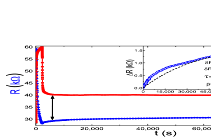
Figure 12: A two-temperatures annealing protocol. The sample, 92nm thick, is heated to T${}_{\text{A}}$=347$\pm$2K for 1300s and then the temperature is changed to 316$\pm$1K. The ensuing R(t) in this case is monotonic. Presumably the amplitude of the annealing component at 316K is insufficient to overcome the effect of recovery associated with the drop from the higher temperature. The inset shows the recovered resistance starting from the point (marked by the arrow in the main figure) where the sample temperature stabilized at T=316K. The dashed line is the best fit to the asymptotic region of the relaxation based on Eq.3.

The difference from the behavior that ensues when T${}_{\text{A}}$ is switched to T${}_{\text{P}}$ as in the previous cases above (rather than to T${}_{\text{I}}$ in Fig.12), is in the functional dependence of R(t). As the inset to Fig.12 shows, $\Delta$R(t) cannot be fitted to a single-component mechanism over the entire time-interval where the sample was already at a constant temperature. This is in contrast to the resistance-relaxation curves in figures 2, 4, and 5 that yielded reasonably good fit to a stretched-exponential time-dependence.

These examples make it clear that the position in time of the peak resistance in the non-monotonous R(t) is a compounded result of the two temperatures used in the protocol and the time spent in each.

This behavior is quite different than that observed in the electron-glass where a memory of time spent under a specific gate-voltage 25 or under a specific longitudinal-field 26 may be simply reflected in post relaxation. This difference is presumably related to the irreversible changes that occur when applying $\Delta$T or pressure on structural glasses. It would be interesting to see if something like the ‘simple-aging’ exhibited by the electron-glass 25 ; 26 may be observed in structural glasses if the pressure is limited to the ‘elastic’ regime. The logic of the heuristic picture described above suggests that the limits of elasticity must also be set by the time the pressure is acting on the system rather than just by its value. Besides a test of our picture, such experiments may be useful to shed light on the microscopics involved in the mechanical properties of amorphous solids.

I.5 1/f noise measurements at different annealing stages

Some aspects of the results of noise measurements presented below were the motivation of this study. There is now however another reason to look at the outcome of these experiments: The S-D picture described above associates densification with modification of some two-state systems. These local structures are often cited as the building-blocks of 1/f-noise 27 ; 28 , among other properties of disordered systems. It is then natural to find out how flicker-noise is affected by the thermal-annealing process.

The noise experiments involved a series of consecutive annealing cycles using three different batches of In${}_{\text{x}}$O films. In each annealing stage the sample was held at progressively increasing temperature T${}_{\text{A}}$ for a dwell-time of the order of $\approx$20 hours. T${}_{\text{A}}$ was chosen such that the resulting resistance after cooldown to room-temperature, where the noise measurement was performed, would decrease by a factor of $\approx$2. As a rule of thumb, for most of the resistance range, this requires tuning the heating-power such that the sample resistance at the beginning of the heating-period is $\approx$1/3 of its initial value. Noise measurements were taken about one hour after the sample reached room temperature. In each annealing stage 10${}^{\text{3}}$ time-sweeps were taken to get a well-averaged power spectrum over the frequency range 2-802 Hz. To check on time dependence, another 10${}^{\text{3}}$ time-sweeps were taken 20 minutes after the first set to compare with the first result. Noise spectra for two resistances in an annealing series pertaining to one of the batches studied are shown in Fig.13.

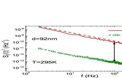
Figure 13: The noise power-spectrum for two resistances in the annealing series of a 92nm thick samples. The dashed line depicts a 1/f law for comparison. The arrow indicates the frequency at which the magnitude of the noise was taken for the plot in Fig.14.

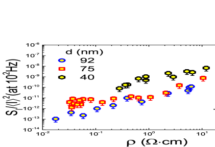
Figure 14: The normalized noise magnitude (estimated at f=100Hz, see Fig.13) as function of the sample resistivity. The three batches of samples that were studied in this part are labelled by their thickness.

These traces exhibit a 1/f character except that they are slightly convex towards the origin of the axis, a shape that characterized all our samples independent of resistance. Data for the noise magnitude as function of resistivity are shown in Fig.14 for the three batches of samples studied in this work. Overall, there is a monotonic increase of S${}_{\text{I}}$/$\langle$I${}^{\text{2}}\rangle$ with the sample resistivity $\rho$ but with a considerable scatter of the data points; a factor of $\approx$5 difference in magnitude between two consecutive measurements on the same sample was encountered in some cases. Common artifacts relating to the measuring circuits, non-linear effects, contacts etc. were ruled out. These large fluctuations in the noise magnitude are apparently peculiar to non-Gaussianity, and are often seen in 1/f studies of disordered systems 28 ; 29 ; 30 ; 31 . One may suspect that the long-lasting non-equilibrium nature of R(t) following the annealing protocol is responsible for the deviation from a Gaussian noise 28 . This issue clearly deserves further study.

The decrease on the noise magnitude with annealing may be the expected result. Annealing is intuitively associated with removal of defects which naturally contribute to scattering and therefore smaller resistance results in the process. However, the experimental evidence for the structural changes only supports a volume shrinkage that in turn leads to diminishment of the off-diagonal disorder and broadening of the conduction band 14 . The modification of S-states to D-states in the densification process would not necessarily influence the magnitude of the 1/f-noise either, at least not in the frequency window probed in Fig.13. It should be noted that noise magnitude proportional to the sample resistance has been observed in at least two other systems: YBa${}_{\text{2}}$Cu${}_{\text{3}}$O${}_{\text{7-}\delta}$ 31 and in some organic-composite system 33 . The resistance is these systems was changed by a variety of means; temperature, gate-voltage, oxygen-contents (YBa${}_{\text{2}}$Cu${}_{\text{3}}$O${}_{\text{7-}\delta}$), and by the relative composition of the conducting compound in the organic system 33 . In our study, the system resistance was changed by yet another means - densification. The intriguing result is that in all these cases, independent of the material and of the way that the resistance is changed one gets the same simple S${}_{\text{I}}$/$\langle$I${}^{\text{2}}\rangle\propto$R relation. As far as we can see, the one common feature in these experiments is that the studied systems were all in the insulating regime. It is therefore tempting to look for the origin of this result in the general transport properties of the hopping regime. For example, it is well known that the flicker-noise magnitude depends on the volume of the sample 27 ; 28 . In the hopping regime, the effective volume of the system depends on the current-carrying network which typically occupies a small part of the physical structure and, in particular, it depends on temperature and disorder 34 . The volume associated with this network increases as the system approaches the diffusive regime and its resistance becomes smaller. Larger effective volume leads to a better ensemble averaging of the contribution of local fluctuators and thus smaller noise-amplitude. A percolation treatment of this problem, probably incorporating correlations effects 35 will be needed to find out whether this may lead to the observed simple scaling of the noise magnitude with the resistance. On the experimental side it would be helpful to test other systems in order to check on the generality of the relation.

II Summary

We have shown in this work that structural changes that occur during thermal-annealing of In${}_{\text{x}}$O films can be observed in real time by monitoring the system resistance and optical properties. Using these techniques allow tracking of the dynamics and energetics associated with these phenomena during densification, and after its termination while the system relaxes towards a new (metastable) state. These processes are activated and exhibit temporal dependencies that fit the Kohlrausch-law often encountered in experiments involving slow-dynamics of structural glasses.

Many of the effects produced by thermal-annealing on In${}_{\text{x}}$O films were observed in high-pressure densification experiments on a number of amorphous systems. We have argued that these similarities may be accounted for by assuming a simple form for the interparticle potential. A detailed study of the dynamic associated with pressure densification should offer a stringent test of how generic this picture may actually be. Measuring the influence of the time spent under a constant pressure on the temporal behavior and magnitude of the recovered volume after the pressure is released should give valuable information on these issues.

Densification by thermal-treatment may be an effective way to shed light on some of the fundamental properties of amorphous systems. In particular, this technique may be used to tweak the ‘Boson-peak’, one of the most renowned earmarks of glasses. This feature appears as an enhanced density of low-frequency vibrations relative to the Debye spectrum. The Boson-peak has been conjectured to be linked to the rarefied structure 36 and the distributed nature of the interparticle separation characterizing the disordered solid 37 . More recently, it has been conjectured to be responsible for the dominance of the Kohlrausch-law 18 in glassy dynamics. The flexibility of thermal-annealing in controlling densification makes it a prime tool for testing these ideas.

- (1) P. W. Bridgman and I. Šimon, J. of Appl. Phys., 24, 405 (1953).
- (2) S. Sakka and J. D. Mackenzie, J. of Non-Crys Sol., 1, 107 (1969).
- (3) J. D. Mackenzie, J. of Am. Ceramic Soc., 46. 461 (1963).
- (4) J. D. Mackenzie, J. of Am. Ceramic Soc., 46, 470 (1963).
- (5) Wu and H.L. Luo, Journal of Non-Crystalline Solids 18, 21 (1975).
- (6) N. Sakai and H. Fritzsche, Phys. Rev. B 15, 973 (1977).
- (7) Seinosuke Onari, Takao Inokuma, Hiromichi Kataura, and Toshihiro Arai, Phys. Rev. B 35, 4373 (1987).
- (8) A. Polian and M. Grimsditch, Phys. Rev. B 41, 6086 (1990).
- (9) S. Susman, K. J. Volin, D. L. Price, M. Grimsditch, J. P. Rino, R. K. Kalia, and P. Vashishta, G. Gwanmesia, Y. Wang, and R. C. Liebermann, Phys. Rev. B 43, 1194 (1991).
- (10) Norio Ookubo, Yasuhiro Matsuda, and Noritaka Kuroda, Applied Physics Lett., 63, 346 (1993).
- (11) Daniel J. Lacks, Phys. Rev. Lett., 30, 5385 (1998).
- (12) K. Miyauchi, J. Qiu, M. Shojiya, Y. Kawamoto, N. Kitamura, J. of Non-Crys Sol., 279, 186 (2001).
- (13) V. V. Brazhkin, E. Bychkov, and O. B. Tsiok, Phys. Rev. B 95, 054205 (2017).
- (14) Z. Ovadyahu , Phys. Rev. B. 95, 134203 (2017).
- (15) Z. Ovadyahu, J. Phys. C: Solid State Phys., 19, 5187 (1986).
- (16) U. Givan and Z. Ovadyahu, Phys. Rev. B 86, 165101 (2012); D. Shahar and Z. Ovadyahu, Phys. Rev. B 46, 10917 (1992).
- (17) C. A. Angell, K. L. Ngai, G. B. McKenna, P. F. McMillan, and S. W. Martin, J. of Appl. Phys., 88, 3113 (2000).
- (18) Bingyu Cui, Rico Milkus, and Alessio Zaccone, Phys. Rev. E 95, 022603, (2017).
- (19) E. W. Montroll, J. T. Bendler, J. Stat. Phys. 34,129 (1984); R. G. Palmer, D. L. Stein, E. Abrahams, and P. W. Anderson, Phys. Rev. Lett., 53, 958 (1984); J. S. Langer, S. Mukhopadhyay, Phys. Rev. E 77, 061505 (2008); J.C. Phillips, Rep. Prog. Phys. 59, 1133 (1996); I.M. Lifshitz, Usp. Fiz. Nauk 83, 617 (1964) [Engl. trans. Sov. Phys. Usp. 7, 549 (1965)]; R. Friedberg, J. M. Luttinger, Phys. Rev. B 12, 4460 (1975); P. Grassberger, I. Procaccia, J. Chem. Phys. 77, 6281 (1982).
- (20) D. C. Johnston, Phys. Rev. B 74, 184430 (2006).
- (21) Z. Ovadyahu, Phys. Rev. Lett., 115, 046601 (2015) and references therein.
- (22) P. W. Anderson, B. Halperin C.M. Varma, Phil. Mag. 25, 1 (1972).
- (23) W. A. Phillips, Rep. Prog. Phys. 50, 1657 (1987).
- (24) Z. Ovadyahu, B. Ovryn and H.W. Kraner, J. Elect. Chem. Soc. 130, 917 (1983).
- (25) A. Vaknin, Z. Ovadyhau, and M. Pollak, Phys. Rev. Lett., 84, 3402 (2000).
- (26) V. Orlyanchik, and Z. Ovadyahu, Phys. Rev. Lett., 92, 066801 (2004).
- (27) P. Dutta, and P. M. Horn, Rev. Mod. Phys. 53, 497 (1981).
- (28) M. B. Weissman, Rev. Mod. Phys., 60, 537 (1988).
- (29) C. E. Parman, N. E. Israeloff, and J. Kakalios, Phys. Rev. Lett., 69 1099 (1992).
- (30) Paul A. W. E. Verleg and Jaap I. Dijkhuis, Phys. Rev., B 58, 3904 (1998).
- (31) F. P. Milliken and R. H. Koch, Phys. Rev., B 64, 014505 (2001).
- (32) I. Balberg, Phil. Mag. B, 80, 691 (2000).
- (33) Younggul Song, Hyunhak Jeong, Jingon Jang, Tae-Young Kim, Daekyoung Yoo, Youngrok Kim, Heejun Jeong, and Takhee Lee, AcsNano, 9, 7697 (2015).
- (34) V. Orlyanchik and Z. Ovadyahu, Phys. Rev. B 72, 024211 (2005); ibid, Phys. Rev. B 75, 174205 (2007).
- (35) Kuljinder S. Chase and D. J. Thouless, Phys. Rev. B 39, 9809 (1989).
- (36) Walter Schirmacher, Gregor Diezemann, and Carl Ganter, Phys. Rev. Lett. 81, 136 (1998).
- (37) Hiroshi Shintani and Hajime Tanaka, nature materials 7, 870 (2008).