Solution of parabolic free boundary problems using transmuted heat polynomials

Abstract

A numerical method for free boundary problems for the equation

$$u_{xx}-q(x)u=u_{t}$$ (1)

is proposed. The method is based on recent results from transmutation operators theory allowing one to construct efficiently a complete system of solutions for equation (1) generalizing the system of heat polynomials. The corresponding implementation algorithm is presented.

1 Introduction

Free boundary problems (FBPs) for parabolic equations are of considerable interest in physics (e.g., the Stefan problem) and in financial mathematics (e.g., the problem of pricing of an American option). One of the relatively simple and practical methods proposed for solving FBPs involving the heat equation is the heat polynomials method (see [3], [31], [4], [30], [35], [11]) based on the fact that the system of the heat polynomials represents a complete family of solutions of the heat equation. In the book [3] D. Colton proposed to extend this method onto parabolic equations with variable coefficients by constructing an appropriate transmutation operator and obtaining with its aid the corresponding transmuted heat polynomials. However, the construction of the transmutation operator is a difficult problem itself. In the present work we show that the transmuted heat polynomials required for Colton’s approach can be constructed without knowledge of the transmutation operator by a simple and robust recursive integration procedure. To this aim a recent result from [2] concerning a mapping property of the transmutation operators is used.

This makes possible to extend the heat polynomials method onto equations of the form

$$u_{xx}-q(x)u=u_{t}.$$ (2)

We mention that linear parabolic equations of a more general form with coefficients depending on one variable reduce to (2) (see, e.g., [3, Chap. 2] or [27]).

Thus, we propose a numerical method for approximate solution of a class of FBPs involving (2). This method of transmuted heat polynomials will be designated by THP. The main aim of this paper is to explain it in detail and to propose a simple to implement algorithm for its application.

The subject of FBPs appears in many different fields and applications, as such, presents a large variety of formulations and still open questions. We will not be focusing on the existence and uniqueness of the solution in this paper assuming that it exists in the classical sense.

The paper is structured as follows. In Section 2 we state the FBP. In Section 3 we define transmutation operators and present some of their properties motivating the development of the THP method. In Section 4 we construct the conceptual algorithm for the implementation of the THP method for solving FBPs. In Section 5 we consider an example with an exact solution, with its aid we illustrate the performance of the method. In Section 6 we discuss the possibilities of generalization of our construction and its application to more general FBPs.

2 Statement of the problem

Consider the differential expression

$$\mathbf{A}=\frac{\partial^{2}}{\partial x^{2}}-q(x)$$

with $q\in C[0,L]$, $q:[0,L]\rightarrow\mathbb{C}$.

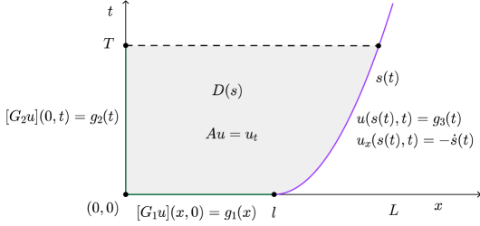
Figure 1: Illustration of Problem 1 statement

Every $s\in C^{1}[0,T]$, such that $0<s(x)\leq L$ for all $x\in[0,T)$ and $s(0)=l$, defines a domain

$$D(s)=\left\{(x,t)\in\mathbb{R}^{2}:0<x<s(t),0<t<T\right\},$$ (3)

see Figure 1. Consider the first order linear differential operators $\mathbf{G}_{1}=\gamma_{11}(x)+\gamma_{12}(x)\frac{\partial}{\partial x}$ and $\mathbf{G}_{2}=\gamma_{21}(t)+\gamma_{22}(t)\frac{\partial}{\partial x}$ , where $\gamma_{ij}$ are some given continuous functions.

Problem 1

Find functions $(u,s)$ such that

(i)

$s\in C^{1}[0,T]$ and such that $0<s(x)\leq L$ for all $x\in[0,T)$ and $s(0)=l$,

(ii)

$u\in C^{2,1}\bigl{(}D(s)\bigr{)}$,

(iii)

the following equation is satisfied on $D(s)$

$$\mathbf{A}u(x,t)=u_{t}(x,t),\qquad(x,t)\in D(s),$$ (4)

(iv)

and the following boundary conditions are satisfied

$$\left[\mathbf{G}_{1}u\right](x,0) =g_{1}(x),\qquad x\in(0,l),\qquad l\leq L,$$ (5)

$$\left[\mathbf{G}_{2}u\right](0,t) =g_{2}(t),\qquad t\in(0,T),$$ (6)

$$u\bigl{(}s(t),t\bigr{)} =g_{3}(t),\qquad t\in(0,T),$$ (7)

$$u_{x}\bigl{(}s(t),t\bigr{)} =-\dot{s}(t),\qquad t\in(0,T),$$ (8)

here the dot over the function $s$ means the derivative with respect to the variable $t$. The last condition is usually known as the equation of heat balance or as the Stefan condition.

This problem is broadly studied in literature (see, e.g., [8], [34], [6], [26], [7] and [36] for additional bibliography). In particular, the classical one dimensional one phase Stefan problem is a special case of Problem 1. Since the subject of this paper is the approximate numerical method for solution of Problem 1, we make the following assumption.

Assumption 2

There exists a unique solution to Problem 1.

A relevant example of an existence and uniqueness result is given in [7, Theorem 1], see Remark 11 below.

3 Transmuted heat polynomials

3.1 Heat polynomials

The heat polynomials are defined for $n\in\mathbb{N}_{0}$ as (see, e.g., [32] and [37])

$$h_{n}(x,t)=\sum_{k=0}^{\left[n/2\right]}c_{k}^{n}x^{n-2k}t^{k},\qquad\text{where }c_{k}^{n}=\frac{n!}{(n-2k)!k!}$$

and $\left[\cdot\right]$ denotes the entire part of the number. The first five heat polynomials are

$$h_{0}(x,t) =1,\qquad h_{1}(x,t)=x,\qquad h_{2}(x,t)=x^{2}+2t,$$

$$h_{3}(x,t) =x^{3}+6xt,\qquad h_{4}(x,t)=x^{4}+12x^{2}t+12t^{2}.$$

The set of the heat polynomials $\left\{h_{n}\right\}_{n\in\mathbb{N}_{0}}$ represents a complete system of solutions for the heat equation

$$u_{xx}=u_{t}$$

on any domain $D(s)$ defined by (3) (see [5]).

3.2 Formal powers and the transmutation operator

Let $f$ be a nonvanishing (in general, complex valued) solution of the equation

$$\left(\frac{d^{2}}{dx^{2}}-q(x)\right)f(x)=0,\qquad x\in(0,L),$$ (9)

such that

$$f(0)=1.$$ (10)

The existence of such solution for any complex valued $q\in C[0,L]$ was proved in [19] (see also [1]).

Consider two sequences of recursive integrals (see [15], [16], [19])

$$X^{(0)}(x)\equiv 1,\qquad X^{(n)}(x)=n\int_{0}^{x}X^{(n-1)}(s)\left(f^{2}(s)\right)^{(-1)^{n}}\,\mathrm{d}s,\qquad n=1,2,\ldots$$

and

$$\widetilde{X}^{(0)}\equiv 1,\qquad\widetilde{X}^{(n)}(x)=n\int_{0}^{x}\widetilde{X}^{(n-1)}(s)\left(f^{2}(s)\right)^{(-1)^{n-1}}\,\mathrm{d}s,\qquad n=1,2,\ldots.$$

Definition 3

The family of functions $\left\{\varphi_{n}\right\}_{n=0}^{\infty}$ constructed according to the rule

$$\varphi_{n}(x)=\begin{cases}f(x)X^{(n)}(x),&n\text{ odd},\\ f(x)\tilde{X}^{(n)}(x),&n\text{ even},\end{cases}$$ (11)

is called the system of formal powers associated with $f$.

The formal powers arise in the spectral parameter power series (SPPS) representation for solutions of the Sturm-Liouville equation, see [14], [19], [12], [16].

The following result from [25] (see also [17] and [21] for additional details) and from [2] guarantees the existence of a transmutation operator associated with $f$ and shows its connection with the system of formal powers.

Theorem 4

Let $q\in C[0,L]$. Then there exists a unique complex valued function $K(x,y)\in C^{1}\bigl{(}[0,L]\times[-L,L]\bigr{)}$ such that the Volterra integral operator

$$\mathbf{T}u(x)=u(x)+\int_{-x}^{x}K(x,y)u(y)\,dy$$

defined on $C[0,L]$ satisfies the equality

$$\mathbf{AT}[u]=\mathbf{T}\left[\frac{d^{2}u}{dx^{2}}\right]$$

for any $u\in C^{2}[0,L]$ and

$$\mathbf{T}\left[1\right]=f.$$

Note that if $v=\mathbf{T}u$ then $v(0)=u(0)$ and $v^{\prime}(0)=u^{\prime}(0)+f^{\prime}(0)u(0)$.

Theorem 5 ([2])

$$\mathbf{T}\left[x^{n}\right]=\varphi_{n}(x)\qquad\text{for any }n\in\mathbb{N}_{0}.$$

3.3 Construction of the transmuted heat polynomials

Denote $H_{n}=\mathbf{T}\left[h_{n}\right]$. Thus, $H_{n}(x,t)=h_{n}(x,t)+\int_{-x}^{x}K(x,y)h_{n}(y,t)\,dy$. The functions $H_{n}$ are called the transmuted heat polynomials [18].

We have $\left(\mathbf{A}-\frac{\partial}{\partial t}\right)H_{n}=\mathbf{AT}h_{n}-\frac{\partial}{\partial t}\mathbf{T}h_{n}=\mathbf{T}\left(\frac{\partial^{2}}{\partial x^{2}}-\frac{\partial}{\partial t}\right)h_{n}=0$ and hence every $H_{n}$ is a solution of the equation

$$\mathbf{A}u=u_{t}.$$ (12)

The set $\left\{H_{n}\right\}_{n\in\mathbb{N}_{0}}$ is a complete system of solutions of (12) in the following sense.

Proposition 6

Let $u$ be a classical solution of (12) in $D(s)$, continuous in the closure $\bar{D}(s)$. Then for any compact set $D_{c}\subset D(s)$ and any given $\varepsilon>0$ there exist $N$ and constants $a_{0},\ldots,a_{N}$ such that

$$\max_{(x,t)\in D_{c}}\left|u(x,t)-\sum_{n=0}^{N}a_{n}H_{n}(x,t)\right|<\varepsilon.$$

Moreover, if $s(t)$ can be extended to a function analytic in the disk $\{t\in\mathbb{C}:|t|\leq T\}$, the uniform approximation property is valid on the whole set $\bar{D}$.

Proof. Suppose first that $q\in C^{1}[0,L]$. Note that any compact set $D_{c}$ can be covered by a subset $D_{a}\subset\bar{D}(s)$ of the form $D_{a}=\{(x,t)\in\mathbb{R}^{2}:0\leq x\leq x_{1}(t)\leq s(t),\ 0\leq t\leq T\}$ with analytic function $x_{1}(t)$. For the set $D_{a}$ the proof is completely similar to that of [3, Theorem 2.3.3] with the only change that the transmutation operator $\mathbf{T}$ and its inverse are used. For the general case $q\in C[0,L]$ one approximates $q$ by a $C^{1}$ function.   

Theorem 7

The transmuted heat polynomials admit the following form

$$H_{n}(x,t)=\sum_{k=0}^{\left[n/2\right]}c_{k}^{n}\varphi_{n-2k}(x)t^{k}.$$

Proof. This equality is an immediate corollary of Theorem 5. Indeed, we have $H_{n}(x,t)=\mathbf{T}h_{n}(x,t)=\sum_{k=0}^{\left[n/2\right]}c_{k}^{n}\mathbf{T}\left[x^{n-2k}\right]t^{k}$, where Theorem 5 is used.   

The explicit form of the functions $H_{n}$ presented in this theorem makes possible the construction of the approximate solution to Problem 1 by the THP method.

4 Description of the method

We proceed to the step by step construction of the THP method, summarizing the algorithm at the end of the section.

Assume that we have already calculated the formal powers $\varphi_{k}$ and the functions $H_{n}$. Further, let $N$ be the highest index of the formal power considered, or equivalently the highest degree in $x$ of the considered heat polynomials. We denote by

$$u_{N}(x,t)=\sum_{n=0}^{N}a_{n}H_{n}(x,t)$$ (13)

the approximation of the solution $u(x,t)$, and by $\bar{a}=\left(a_{0},...,a_{N}\right)^{T}$ the column-vector of the unknown coefficients. Note that by construction functions $u_{N}$ satisfy equation (4), all we need is to find suitable coefficients $\bar{a}$.

Denote by $\left\{t_{i}\right\}$ an ordered set of $N_{t}+1$ points of the interval $[0,T]$, with $t_{0}=0<t_{1}<...<t_{N_{t}}=T$, $\bar{t}=\left(t_{0},...,t_{N_{t}}\right)^{T}$, and by $\left\{x_{i}\right\}$ an ordered set of $N_{x}+1$ points of the initial boundary, with $x_{0}=0<x_{1}<...<x_{N_{x}}=l$, $\bar{x}=\left(x_{0},...,x_{N_{x}}\right)^{T}$.

Consider a set of $K+1$ linearly independent differentiable functions, $\beta_{k}:[0,T]\rightarrow\mathbb{R}$. We are looking for the free boundary in the form

$$s_{K}(t)=\sum_{k=0}^{K}b_{k}\beta_{k}(t).$$

Denote the vector of the unknown coefficients by $\bar{b}=\left(b_{0},...,b_{K}\right)^{T}$. For any function $v$ defined on the set of points $\left\{y_{i}\right\}_{i=0,1,...,N_{y}}$ the following notation is introduced

$$v\left(\bar{y}\right)=\bigl{(}v\left(y_{0}\right),...,v\left(y_{N_{y}}\right)\bigr{)}^{T}.$$

A numerical approximation problem consists in finding a set of the coefficients $\left(\bar{a},\bar{b}\right)$ that best fits the conditions of Problem 1 with the following norm chosen

$$\left\|v(\bar{y})\right\|^{2}=\sum_{i=0}^{N_{y}}|v(y_{i})|^{2}.$$

The following magnitudes are to be minimized,

$$I_{1}\left(\bar{a},\bar{b}\right) =\left\|\left[\mathbf{G}_{1}u_{N}\right]\left(\bar{x},0\right)-g_{1}(\bar{x})\right\|,$$

$$I_{2}\left(\bar{a},\bar{b}\right) =\left\|\left[\mathbf{G}_{2}u_{N}\right]\left(0,\bar{t}\right)-g_{2}(\bar{t})\right\|,$$

$$I_{3}\left(\bar{a},\bar{b}\right) =\left\|u_{N}\bigl{(}s_{K}\left(\bar{t}\right),\bar{t}\bigr{)}-g_{3}(\bar{t})\right\|,$$

$$I_{4}\left(\bar{a},\bar{b}\right) =\left\|\left(u_{N}\right)_{x}\bigl{(}s_{K}\left(\bar{t}\right),\bar{t}\bigr{)}+\dot{s}_{K}(\bar{t})\right\|.$$

Each of them is related to a boundary condition from (5)–(8). With introduction of the value function

$$F\left(\bar{a},\bar{b}\right)=\sum_{i=1}^{4}I^{2}_{i}\left(\bar{a},\bar{b}\right),$$ (14)

the minimization problem can be stated as follows.

Problem 8

Find

$$\underset{\left(\bar{a},\bar{b}\right)}{\arg\min}\,F\left(\bar{a},\bar{b}\right),$$

subject to

$$0<s_{K}(t)\leq L,\qquad t\in[0,T].$$ (15)

Note that instead of the uniform norm chosen in [31] for the heat polynomials method, we used the $L_{2}$ norm in the value function (14). The main reason for such choice was to take advantage of the presence of the so-called separable linear parameters (see [33, Chap. 6.2], see also [10]) and to reduce the number of parameters in the value function. Indeed, for each fixed $\bar{b}$, the constrained minimization Problem 8 reduces to an unconstrained linear least squares problem for parameters $\bar{a}$ and can be easily solved exactly (see Subsection 4.1). That is, for each $\bar{b}$ we can define

$$\bar{a}(\bar{b}):=\underset{\bar{a}}{\arg\min}\,F\left(\bar{a},\bar{b}\right).$$ (16)

So instead of minimizing the value function $F$ over an $N+K+2$ dimensional space of parameters $(\bar{a},\bar{b})$, the problem can be reduced to minimization of the function

$$\tilde{F}(\bar{b}):=F\bigl{(}\bar{a}(\bar{b}),\bar{b}\bigr{)}$$

over a $K+1$ dimensional space. Such reformulation of the original optimization problem leads to a more robust convergence of numerical optimization algorithms, c.f., [10]. We state this new minimization problem as follows.

Problem 9

Find

$$\underset{\bar{b}}{\arg\min}\,\tilde{F}\left(\bar{b}\right)$$

subject to

$$0<s_{K}(t)\leq L,\qquad t\in[0,T].$$ (17)

4.1 Linear minimization problem

Let a vector $\tilde{b}$ be fixed. We have to solve the linear least squares problem (16). Let us denote the corresponding approximate boundary by $\tilde{s}$,

$$\tilde{s}(t)=\sum_{i=0}^{N_{\beta}}\tilde{b}_{i}\beta_{i}(t).$$

Note that problem (16) is equivalent to solving the overdetermined system of linear equations (resulting from the boundary conditions (5)–(8))

$$\left[\mathbf{G}_{1}u_{N}\right]\left(\bar{x},0\right) =\sum_{n=0}^{N}a_{n}B_{n}\left(\bar{x}\right), u_{N}\bigl{(}\tilde{s}\left(\bar{t}\right),\bar{t}\bigr{)} =\sum_{n=0}^{N}a_{n}D_{n}\left(\bar{t}\right),$$

$$\left[\mathbf{G}_{2}u_{N}\right]\left(0,\bar{t}\right) =\sum_{n=0}^{N}a_{n}C_{n}\left(\bar{t}\right), \left(u_{N}\right)_{x}\bigl{(}\tilde{s}\left(\bar{t}\right),\bar{t}\bigr{)} =\sum\limits_{n=0}^{N}a_{n}E_{n}\left(\bar{t}\right),$$

where

$$B_{n}\left(\bar{x}\right) =\begin{cases}c_{0}^{n}\gamma_{11}(\bar{x})\varphi_{n}(\bar{x})+c_{\frac{n-1}{2}}^{n}\gamma_{12}(\bar{x})\varphi_{1}^{\prime}(\bar{x}),&n\text{ odd},\\ c_{0}^{n}\gamma_{11}(\bar{x})\varphi_{n}(\bar{x}),&n\text{ even},\end{cases}$$ (18)

$$C_{n}\left(\bar{t}\right) =\begin{cases}c_{\frac{n-1}{2}}^{n}\gamma_{22}(\bar{t})\bar{t}^{\frac{n-1}{2}},&n\text{ odd},\\ c_{\frac{n}{2}}^{n}\gamma_{21}(\bar{t})\bar{t}^{\frac{n}{2}},&n\text{ even},\end{cases}$$ (19)

$$D_{n}(\bar{t}) =\sum_{k=0}^{[n/2]}c_{k}^{n}\varphi_{n-2k}(\tilde{s}(\bar{t})\bar{t}^{k},\qquad E_{n}(\bar{t})=\sum_{k=0}^{[n/2]}c_{k}^{n}\varphi_{n-2k}^{\prime}(\tilde{s}(\bar{t}))\bar{t}^{k},$$ (20)

or in the matrix form

$$\mathbf{B}\bar{a}\simeq\mathbf{g},$$ (21)

where

$$\mathbf{B}=\begin{pmatrix}B_{0}(\bar{x})&\dots&B_{N}\left(\bar{x}\right)\\ C_{0}(\bar{t})&\dots&C_{N}\left(\bar{t}\right)\\ D_{0}(\bar{t})&\dots&D_{N}\left(\bar{t}\right)\\ E_{0}(\bar{t})&\dots&E_{N}\left(\bar{t}\right)\end{pmatrix}\qquad\text{and}\qquad\mathbf{g}=\begin{pmatrix}g_{1}(\bar{x})\\ g_{2}(\bar{t})\\ g_{3}(\bar{t})\\ \dot{\widetilde{s}}(\bar{t})\end{pmatrix}.$$

Note that the derivatives $\varphi^{\prime}$ in (20) do not require numerical differentiation and can be obtained in a closed form from (11).

The solution of this overdetermined system coincides [24, Thm. 5.14] with the unique solution of the following fully determined system of linear equations

$$\mathbf{C}\bar{a}=\mathbf{h},\qquad\text{where }\mathbf{C}=\mathbf{B}^{T}\mathbf{B}\text{ and }\mathbf{h}=\mathbf{B}^{T}\mathbf{g}.$$ (22)

See also [23] or [28] for various methods of efficient solution of equation (21) or (22). In particular, we used the Moore-Penrose pseudo-inverse method.

4.2 Implementation

Here we present the algorithm of the implementation of the THP method for Problem 1.

1. Find a particular solution of equation (9) satisfying (10). For example, the SPPS method presented in [19] can be used.

2. Construct the formal powers on an interval from $0$ to some $L>l$. In this paper we represented all the functions involved by their values on a uniform mesh and used the Newton-Cotes six point integration rule. Since we may need the values of the formal powers at arbitrary points $\tilde{s}\left(\bar{t}\right)\subset[0,L]$, we approximated the formal powers by splines passing through their values on the selected mesh. Spline integration can be used as well for the construction of the formal powers, c.f., [13]. See also [17] for the discussion of other possible methods.

3. Compute the coefficients $B_{n}$ and $C_{n}$ given by (18) and (19) and the respective functions $g_{1}$ and $g_{2}$. Since these conditions are independent of the free boundary (i.e. of the choice of $\tilde{b}$), they need to be computed only once.

4. Construct a function that solves problem (16) for each given set of coefficients $\tilde{b}$.

5. Construct the value function $\tilde{F}\left(b\right)$ using (14).

6. Solve the constrained minimization Problem 9 using any suitable algorithm, see, e.g., [28]. For the numerical illustration we used the Matlab function fmincon. Note that for faster convergence we may initially solve the minimization Problem 9 for some small value $K^{\prime}<K$ and use the coefficients $b^{0}_{k}$, $k=0,\ldots,K^{\prime}$ obtained as an initial value for the optimization algorithm for larger value $K$.

5 Numerical illustration

5.1 Example with an exact solution and a tractable free boundary

For the numerical experiment we constructed an example of an FBP admitting an exact solution.

For every $s\in C^{1}[0,1]$, with $s(0)=1$ consider the domain

$$D(s)=\left\{(x,t)\in\mathbb{R}^{2}:0<x<s(t),\,0<t<1\right\}.$$

Problem 10

Find the pair $(s,u)$ such that $s\in C^{1}[0,1]$, $u\in C^{2,1}\left(D(s)\right)$ and

$$u_{xx}-x^{2}u=u_{t},\qquad(x,t)\in D(s),$$

with the following boundary conditions

$$u(x,0) =e^{-\frac{x^{2}}{2}}, x\in[0,1],$$ (23)

$$u_{x}(0,t) =0, t\in(0,1),$$ (24)

$$u(s(t),t) =e^{-\operatorname{Ei}^{-1}\left(2C-2e^{-t}\right)-t}, t\in(0,1),$$ (25)

$$u_{x}(s(t),t) =-\dot{s}(t), t\in(0,1),$$ (26)

where

$$C=\frac{1}{2}\operatorname{Ei}\left(\frac{1}{2}\right)+1\approx 1.2271,$$

and $\operatorname{Ei}^{-1}$ stands for the inverse function of the exponential integral $\operatorname{Ei}$,

$$\operatorname{Ei}\left(x\right)=-\operatorname{v.p.}\int_{-x}^{\infty}\frac{e^{-t}}{t}dt.$$

Problem 10 possesses an exact solution $u$ given by

$$u(x,t)=e^{-\frac{x^{2}}{2}-t},\qquad(x,t)\in D(s),$$ (27)

and the free boundary

$$s\left(t\right)=\sqrt{2\operatorname{Ei}^{-1}\left(2C-2e^{-t}\right)},\qquad t\in\left[0,1\right].$$ (28)

Remark 11

The existence and the uniqueness of the solution for $t\in\left[0,1\right]$ is guaranteed by [7, Theorem 1]. For the application of the theorem it is necessary to use the transformation $v(x,t)=u(x,t)+\gamma(t)$, where $\gamma(t)=\exp\left(-\operatorname{Ei}^{-1}\left(2C-2e^{-t}\right)-t\right)$.

5.2 Numerical illustration

We proceed by presenting numerical results delivered by the algorithm described in Section 4. All the calculations were carried out in Matlab R2012a.

A particular solution to equation (9) and the formal powers (11) were represented by their values on a 2000-points uniform mesh. The Newton-Cotes integration rule was used for their computation. The number of formal powers considered was set at $N=12$. Finally the function spapi was used to create splines approximating the formal powers. For computing the $\operatorname{Ei}^{-1}$ we have used a polynomial interpolation on a fine grid for the function $\operatorname{Ei}$. The values for the function $\operatorname{Ei}$ were constructed by the series expansions presented in [9, (8.214)], see also [29].

The sets of points $\left\{t_{i}\right\}$ and $\left\{x_{i}\right\}$ considered are both equidistant grids of $101$ points. The free boundary $s$ is sought in terms of polynomials. The condition $s(0)=1$ inspires the following form

$$s_{K}\left(\bar{t}\right)=1+\sum_{j=1}^{K}b_{j}\bar{t}^{j}.$$

In our calculations we have considered $K=6$.

The linear problem (16) was solved by using the Matlab function pinv. We have found the solution to Problem 9 using the Matlab routine fmincon.

The proposed algorithm converged rapidly for various initial free boundaries tested. On Figure 2 we present one of the initial boundaries, the exact free boundary $s(t)$ calculated from equation (28) and the difference between the exact free boundary $s(t)$ and the obtained approximation $s_{K}(t)$. The obtained approximate boundary was

$$s_{K}(t)=1+0.60657885t-0.30458770t^{2}+0.03631846t^{3}+0.06761711t^{4}-0.05111378t^{5}+0.01270860t^{6},$$ (29)

here and after the coefficients are presented up to the eighth decimal place. The coefficients of the vector $\bar{a}$ that corresponds to the solution of the linear problem (16) with $\bar{b}$ consisting of the coefficients from (29) are

$$a_{0} =1.00000201, a_{1} =-3.88882172\cdot 10^{-6}, a_{2} =-5.00020660\cdot 10^{-1},$$

$$a_{3} =2.67326664\cdot 10^{-5}, a_{4} =4.16822991\cdot 10^{-2}, a_{5} =-2.03778980\cdot 10^{-5},$$

$$a_{6} =-1.38990292\cdot 10^{-3}, a_{7} =4.02691726\cdot 10^{-6}, a_{8} =2.43785480\cdot 10^{-5},$$

$$a_{9} =-2.56424452\cdot 10^{-7}, a_{10} =-2.28538929\cdot 10^{-7}, a_{11} =4.70925279\cdot 10^{-9},$$

$$a_{12} =7.12497038\cdot 10^{-10}.$$

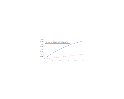
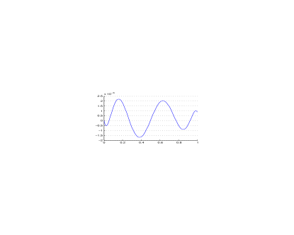
Figure 2: Left: the initial boundary $s_{in}(t)=1+0.1t$ and the exact boundary $s(t)$ for the Problem 10. Right: the difference between the exact boundary $s(t)$ and the approximate boundary $s_{K}(t)$.

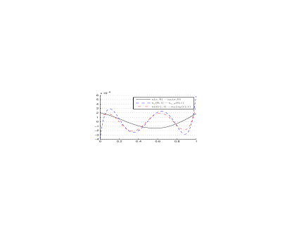
Figure 3: Accuracy of fulfillment of the boundary conditions (23)–(26) for the approximate solution $u_{N}$ and approximate free boundary $s_{K}$ obtained by the algorithm. On the left: conditions (23)–(25), on the right: condition (26).

Figure 3 illustrates the accuracy of fulfillment of the boundary conditions (23)–(26). The absolute value of the difference between the exact solution (27) and the obtained approximate solution in the domain $D(s)$ is presented on Figure 4.

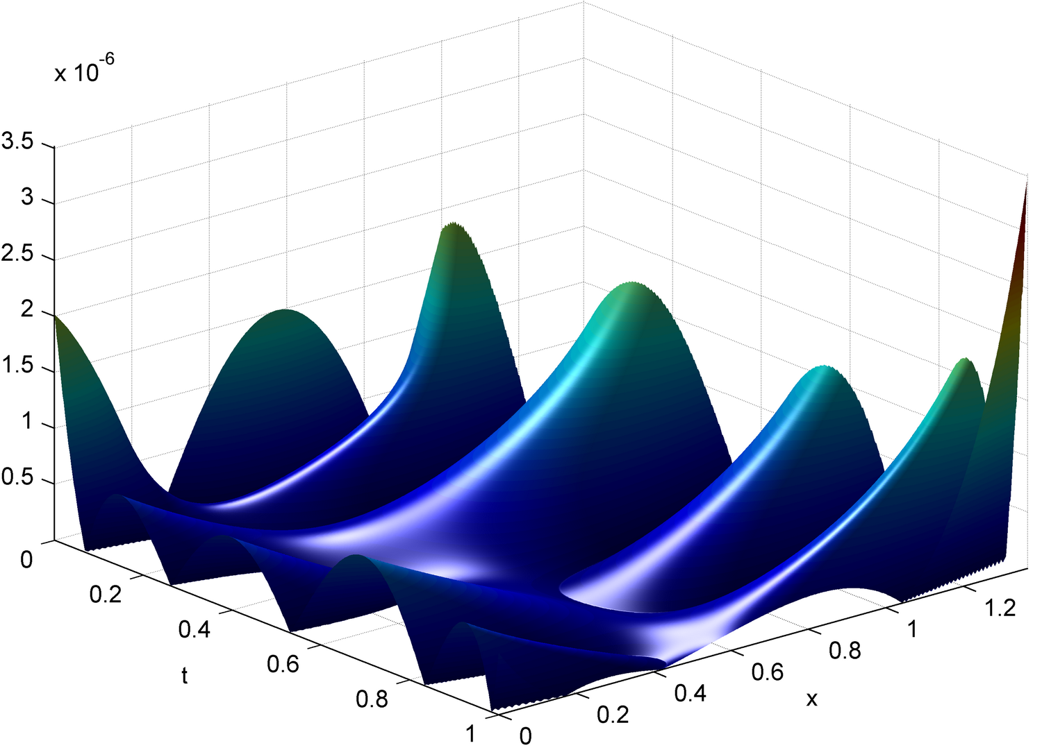
Figure 4: The absolute difference $|u(x,t)-u_{N}(x,t)|$ between the exact and the approximate solutions for the Problem 10 in the domain $D(s)$.

Note that for the problem considered one may look for an approximate solution in the form

$$u_{N}(x,t)=\sum_{n=0}^{N/2}a_{2n}H_{2n}(x,t),$$

i.e., having only even coefficients $a_{2n}$. In such way the boundary condition (24) is satisfied automatically. The proposed algorithm can be applied with minimal modifications for such simplified form of an approximate solution, however we did not observe any gain in the obtained result, the original formulation of the algorithm performed equally well.

6 Possible extensions of the method to more general FBPs and final remarks

6.1 Generalization of the operator $\mathbf{A}$

The presented method can be extended onto operators of the form

$$\mathbf{C}=\alpha_{1}(x)\frac{\partial^{2}}{\partial x^{2}}+\alpha_{2}(x)\frac{\partial}{\partial x}+\alpha_{3}(x)$$

with sufficiently regular coefficients $\alpha_{i}(x)$. For the construction of the formal powers in this case see [22]. The FBPs with this type of operators are very common in financial applications.

6.2 Generalizations of the conditions on a free boundary

6.2.1 Linear generalization

The conditions (7) and (8) are sometimes referred to as Stefan’s conditions. Our algorithm can be applied to more general conditions of the type

$$\mathbf{G}_{3}u(s(t),t) =g_{3}\bigl{(}t,s(t),\dot{s}(t)\bigr{)},$$

$$\mathbf{G}_{4}u(s(t),t) =g_{4}\bigl{(}t,s(t),\dot{s}(t)\bigr{)},$$

for some first order linear differential operators $\mathbf{G}_{3}$ and $\mathbf{G}_{4},$ and where $g_{3}$ and $g_{4}$ are given functions of three variables.

6.2.2 Nonlinear generalization

For some FBPs we can only express the conditions (7) and (8) as

$$g_{3}\bigl{(}t,s(t),\dot{s}(t),u(s(t),t),u_{x}(s(t),t)\bigr{)} =0,$$

$$g_{4}\bigl{(}t,s(t),\dot{s}(t),u(s(t),t),u_{x}(s(t),t)\bigr{)} =0,$$

where $g_{3}$ and $g_{4}$ are given functions of five variables. In this case the elegant decomposition into a linear and nonlinear problems will be lost, however the hierarchic structure of the minimization problem remains, i.e., the minimization Problem 8 can be reduced to the Problem 9 with the only difference that the auxiliary problem (16) may be nonlinear.

6.3 Nonlinear form of the boundary

Often in applications some additional information is available about the free boundary structure. With this additional knowledge (or for other reasons) the linear decomposition of the boundary might not be appropriate. It is easy to see that we can still apply the algorithm assuming that

$$s_{K}=\xi\left(b_{0},...,b_{K}\right),$$

for the known function $\xi$. This nonlinear structure can slow down the algorithm for the search of the minimum in Problems 8 or 9, due to the constraints (15) and (17) respectively. In our particular Matlab implementation, we have used fmincon function that performs better with a linear constraint on the boundary than a nonlinear one.

6.4 Concluding remarks

A method for approximate solution of a large variety of FBPs is proposed. It is based on a possibility to construct a complete system of solutions of a parabolic equation called transmuted heat polynomials. The numerical implementation is relatively simple and direct. The time required for computations is within seconds. The method admits extensions onto a much larger class of FBPs then that discussed in the paper.

References

- [1] R. Camporesi and A. J. Di Scala. A generalization of a theorem of Mammana. In Colloquium Mathematicum, volume 122-2, pages 215–223. Institute Matematyczny PAN, 2011.
- [2] H. M. Campos, V. V. Kravchenko and S. M. Torba. Transmutations, L-bases and complete families of solutions of the stationary Schrödinger equation in the plane. Journal of Mathematical Analysis and Applications, 389(2):1222–1238, 2012.
- [3] D. Colton. Solution of boundary value problems by the method of integral operators. Pitman London, 1976.
- [4] D. Colton and R. Reemtsen. The numerical solution of the inverse Stefan problem in two space variables. SIAM Journal on Applied Mathematics, 44(5):996–1013, 1984.
- [5] D. Colton and W. Watzlawek. Complete families of solutions to the heat equation and generalized heat equation in . Journal of Differential Equations, 25(1):96–107, 1977.
- [6] J. Crank. Free and moving boundary problems. Clarendon press Oxford, 1984.
- [7] A. Fasano and M. Primicerio. Free boundary problems for nonlinear parabolic equations with nonlinear free boundary conditions. Journal of Mathematical Analysis and Applications, 72(1):247–273, 1979.
- [8] A. Friedman. Partial differential equations of parabolic type. Prentice-Hall, Inc., Englewood Cliffs, N.J., 1964.
- [9] I. S. Gradshteyn and I. M. Ryzhik. Table of Integrals, Series, and Products, 7th ed. Academic Press, 2007. Translated from Russian by Scripta Technica, Inc.
- [10] A. Herrera-Gomez and R. M. Porter. Mixed linear-nonlinear least squares regression. arXiv preprint arXiv:1703.04181, 2017.
- [11] S. N. Kharin, M. M. Sarsengeldin, H. Nouri, A. Ashyralyev and A. Lukashov. Analytical solution of two-phase spherical Stefan problem by heat polynomials and integral error functions. In AIP Conference Proceedings, volume 1759-1, 020031, 6 pages. AIP Publishing, 2016.
- [12] K. V. Khmelnytskaya, V. V. Kravchenko and H. C. Rosu. Eigenvalue problems, spectral parameter power series, and modern applications. Mathematical Methods in the Applied Sciences, 38(10):1945–1969, 2015.
- [13] K. V. Khmelnytskaya, V. V. Kravchenko, S. M. Torba and S. Tremblay. Wave polynomials, transmutations and Cauchy’s problem for the Klein–Gordon equation. Journal of Mathematical Analysis and Applications, 399(1):191–212, 2013.
- [14] V. V. Kravchenko. A representation for solutions of the Sturm-Liouville equation. Complex Variables and Elliptic Equations, 53(8):775–789, 2008.
- [15] V. V. Kravchenko. Applied Pseudoanalytic Function Theory. Birkhäuser Basel, 2009.
- [16] V. V. Kravchenko, S. Morelos and S. M. Torba. Liouville transformation, analytic approximation of transmutation operators and solution of spectral problems. Applied Mathematics and Computation, 273:321–336, 2016.
- [17] V. V. Kravchenko, L. J. Navarro and S. M. Torba. Representation of solutions to the one-dimensional Schrödinger equation in terms of Neumann series of Bessel functions. arXiv preprint arXiv:1508.02738, 2015.
- [18] V. V. Kravchenko, J. A. Otero and S. M. Torba. Analytic approximation of solutions of parabolic partial differential equations with variable coefficients. arXiv preprint arXiv:1706.06126, 2017.
- [19] V. V. Kravchenko and R. M. Porter. Spectral parameter power series for Sturm-Liouville problems. Mathematical Methods in the Applied Sciences, 33(4):459–468, 2010.
- [20] V. V. Kravchenko and S. M. Torba. Modified spectral parameter power series representations for solutions of Sturm-Liouville equations and their applications. Applied Mathematics and Computation, 238:82–105, 2014.
- [21] V. V. Kravchenko and S. M. Torba. Analytic approximation of transmutation operators and applications to highly accurate solution of spectral problems. Journal of Computational and Applied Mathematics, 275:1–26, 2015.
- [22] V. V. Kravchenko and S. M. Torba. A Neumann series of Bessel functions representation for solutions of Sturm-Liouville equations. arXiv preprint arXiv:1612.08803, 2016.
- [23] C. L. Lawson and R. J. Hanson. Solving least squares problems, volume 15 of Classics in Applied Mathematics. Society for Industrial and Applied Mathematics (SIAM), Philadelphia, PA, 1995. Revised reprint of the 1974 original.
- [24] K. Madsen and H. Nielsen. Introduction to Optimization and Data Fitting. 2008.
- [25] V. A. Marchenko. Some questions of the theory of one-dimensional linear differential operators of the second order. I. Transactions of Moscow Mathematical Society, 1:327–420, 1952.
- [26] A. M. Meirmanov. The Stefan Problem. Walter de Gruyter, 1992.
- [27] T. Miyazawa. Theory of the one-variable Fokker-Planck equation. Physical Review A, 39(3):1447–1468, 1989.
- [28] J. Nocedal and S. J. Wright. Numerical optimization. Springer, New York, 2006.
- [29] P. Pecina. On the function inverse to the exponential integral function. Bulletin of the Astronomical Institutes of Czechoslovakia, 37:8–12, 1986.
- [30] R. Reemtsen and A. Kirsch. A method for the numerical solution of the one-dimensional inverse Stefan problem. Numerische Mathematik, 45(2):253–273, 1984.
- [31] R. Reemtsen and C. J. Lozano. An approximation technique for the numerical solution of a Stefan problem. Numerische Mathematik, 38(1):141–154, 1982.
- [32] P. C. Rosenbloom and D. V. Widder. Expansions in terms of heat polynomials and associated functions. Transactions of the American Mathematical Society, 92(2):220–266, 1959.
- [33] G. J. S. Ross. Nonlinear estimation. Springer series in statistics. Springer-Verlag, 1990.
- [34] L. I. Rubinshtein. The Stefan problem. American Mathematical Soc. Translations of Mathematical Monographs, Vol. 27, 1971.
- [35] M. M. Sarsengeldin, A. Arynov, A. Zhetibayeva and S. Guvercin. Analytical solutions of heat equation by heat polynomials. Bulletin of National Academy of Sciences of the Republic of Kazakhstan, 5:21–27, 2014.
- [36] D. A. Tarzia. A bibliography on moving-free boundary problems for the heat-diffusion equation. The Stefan and related problems, MAT-Serie A, 2, 2000.
- [37] D. V. Widder. Analytic solutions of the heat equation. Duke Math. J., 29(4):497–503, 1962.