The energy landscape of a simple
neural network

Abstract

We explore the energy landscape of a simple neural network. In particular, we expand upon previous work demonstrating that the empirical complexity of fitted neural networks is vastly less than a naive parameter count would suggest and that this implicit regularization is actually beneficial for generalization from fitted models.

1 Introduction

Neural networks have become very popular due to their ability to fit complicated high dimensional functions (e.g. determining the breed of dog featured in a photo). In many cases, the most successful networks are enormous, with many millions of parameters. Although typical training data sizes are also quite large, the amount of data is often miniscule when the dimension of the feature space is considered or when compared to the theoretical fitting capability of the network. We typically explain away the first issue by observing that the region of interest in a high dimensional feature space is likely to be much lower dimensional, so as long as we have a representative training sample, a fitted model should be accurate where it needs to be. However, we are left with the problem that the networks we use are often much too large, in the sense that they should be capable of completely reproducing the training data. In practice, this does not occur; in other words, this problem is not actually a problem, which leaves us with the question: why?

In [4, 5], we show that random neural networks (which includes standard initialized networks under training) are far less complex than they theoretically could be, and we show that trained neural networks retain this simplicity throughout training. In other words, the answer to the question of why networks do not overfit is:

1. the complexity of a network increases smoothly with training time, and

2. there is an empirical upper bound on complexity which is much less than the theoretical limit.

In this paper, we expand upon (2) and explain why it can be beneficial. Specifically, we will construct a small neural network which is, by design, capable of fitting, but essentially incapable of learning, a given complex “high frequency” function. We study the energy landscape of this network in an effort to understand the distribution and size of the local minima and the general topography of the weight space. We find that local minima are common; the weight space is rough, with many long, flat valleys; and that the domains of attraction of the global minima are very narrow. The global minima in the weight space correspond to a perfect fit of the data, but the local minima correspond to a “de-noised” version of the function which has had the high-frequency components removed. That is, the energy landscape has a regularizing effect, and it is essentially impossible to reach a global minimum while training.

The definition of “noise” is problem dependent: we might want to actually fit the high-frequency components in our example below, and we can do that by increasing the size of the network. Our point is not that networks in general cannot learn the function we construct but that networks large enough to fit the function perfectly might still not be large enough to actually learn it in practice, and when they cannot learn it, they do a good job of learning just the low frequency components.

The paper [2], discovered after the initial draft of this paper was written, also explores the energy landscape of neural networks, although their theme is different from ours. We remark on one point in the conclusion of [2] which appears at odds with our assertion that it can be difficult to find a global minimum or a local minimum which is competitive with it: they observe the opposite; they find it quite easy to find a global minimum. In fact, both observations can be reconciled: Given a trained network, which our previous work has shown is likely to produce smooth (low complexity) output, it should be relatively easy to train a second network to match the output of the first; good local minima for the two networks are likely to be similar. (And randomly-initialized networks tend to produce smooth, low complexity output.) On the other hand, a network constructed (not trained) to produce a specific non-smooth (high complexity) output would be difficult for another network (with the same architecture) to train to.

2 Construction of a perfect fit

Our goal is to exhibit a function and a network structure such that the network can perfectly fit the function but never does under training. Note that the only way to produce such a function is as the output of the network itself, because otherwise, we could never find the perfect fit. For simplicity, we construct a network with one input and one output, and we have $K$ hidden densely connected layers of $N$ nodes each. We call this a $K\times N$ network. The hidden layers all have relu activation, and the output layer has a linear activation. We will carefully construct the weights of the network in two blocks. Choose $N_{1}$ and $N_{2}$ such that $N_{1}+N_{2}=N$. The first block, arbitrarily on the left side of the network, uses $N_{1}$ nodes in each hidden layer to produce a high-frequency sawtooth wave in a manner similar to [3]. The second block, on the right, uses $N_{2}$ nodes in each hidden layer to produce a relatively simple low frequency spline. In fact, we only actually use the first layer on the right: the subsequent layers are the (relued) identity function. The output node simply takes the sum of the high frequency sawtooth and the low frequency spline. We refer to this as a $K\times(N_{1}+N_{2})$ network.

Note that because many nodes on the right are unused, even this network is larger than it needs to be to perfectly fit the output function. For our main working example, we chose a random $5\times(2+3)$ network of this form. We want to construct the smallest possible interesting example, to make numerical study easier, but networks much smaller than the one constructed here tend to be degenerate. See Figure 1 for the network structure and example function. We refer to this output function as $f:\mathbb{R}\to\mathbb{R}$ and the perfect-fit network weights as $W_{f}$.

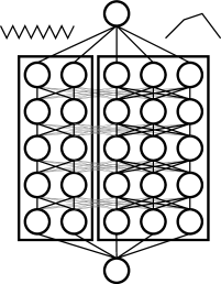
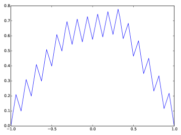
Figure 1: Our main example model, constructed as a sum of a high-frequency sawtooth wave and a low frequency spline (left) and the graph of the output function of this network (right). Our hand-constructed model has nonzero weights only on the bold lines, but the models trained on its output have no constraints on the weights.

Note, though, that when we train a $5\times 5$ model to the output of $W_{f}$, we do not enforce the two sided structure — the network is fully connected on each layer. The $2+3$ format is just the hand crafted way to produce the sum of high and low frequency components.

3 Symmetrization

If two weights $W_{1}$ and $W_{2}$ produce the same output function, we say they are symmetric. The space of weights of a $K\times N$ network has a large group of symmetries. In particular, it contains the group $\mathbb{R}_{+}^{KN}\rtimes S_{N}^{K}$, where $S_{N}$ is the symmetric group on $N$ elements and $\mathbb{R}_{+}$ is the multiplicative group of positive reals. To see this, note that we can rearrange the indices on the hidden nodes at will, producing the group $S_{N}^{K}$, and we can scale up the weights and bias at a particular node, as long as we perform the reciprocal scaling on the associated weights in the next layer up, producing $\mathbb{R}_{+}^{KN}$, and the action of $S_{N}^{K}$ on $\mathbb{R}_{+}^{KN}$ in the semidirect product is the obvious permutation action.

The presence in the symmetry group of $\mathbb{R}_{+}^{KN}$ means that at any point $W$ in weight space, there is a $KN$-dimensional submanifold passing through $W$ along which the output function is completely unchanged, and the presence of the $S_{N}^{K}$ factor means that there are a large number ($(N!)^{K}$) of these submanifolds in weight space, each with identical outputs. There is a question of whether removing all of these symmetries from the weight space will make training easier. See [1], for example, for more background.

Because we are interested in exploring the actual weight space of our network structure and not just the output functions, we introduce a symmetrization procedure, as follows. First, find the element of $\mathbb{R}_{+}^{KN}$ which minimizes the $L_{2}$ norm of the entire weight vector (the “minimal energy weights”), then permute the nodes in each layer so the columns of the weight matrices are in increasing $L_{2}$ norm order.

In our experiments, this procedure, applied after training, tends to make paths in weight space slightly smoother, but it does not appear to fundamentally affect any of the observations which follow. Our main purpose in symmetrizing is that our example network $W_{f}$ weights were constructed by hand, and as such they tend to be rather different from the initialization weights or the weights to which the network trains; in particular, $W_{f}$ contains unusually large values. We want to be fair and explore the neighborhood of the “generic representative” of all networks symmetric to our example, in weight space, and we choose the minimum energy weights as our representative. Hereafter, $W_{f}$ refers to these minimum energy weights, and we find minimum energy representatives for all fitted networks.

We emphasize that this symmetrization does not affect the training of the network: we do no quotienting of the weight space during the training process. It is only afterwards, when we want to explore the weight space, that we choose nice representatives of the fitted networks.

4 Experimental results

4.1 Initial example fit

First, we give an example plot showing our main theme. If one fits a $5\times 5$ network to the function $f$ and trains until the weights appear to stabilize, the fitted network will have output which looks similar to Figure 2. It doesn’t much matter which optimizer one uses or how long one trains.

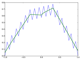
Figure 2: Fitting a network of the same size to the output $f$ of $W_{f}$ (blue) always produces a network with output similar to the green plot.

4.2 Fitting method

All of the models discussed in this paper were trained in the following way, unless otherwise mentioned. Because we know the function we want to fit, exactly, we are in the unusual position of having as much data as we’d like. Our training data consisted of the set of all knots in the linear spline of $f$, plus $9$ points on each of the linear segments between knots; this produces training sets of size $n=32\times 10=320$ points for our principal example. Experimentally, once we provide 2 to 3 points per segment, changing the amount of data has no effect on the results. Indeed, after enough data is provided, the complexity of a trained network is a function of the associated energy landscape. On each training step, we provided this entire dataset to the model, and we used either gradient descent with momentum or adadelta for 50,000 steps.

In practice, it takes only a few hundred steps until the model appears to stabilize with either optimizer. At this point, running gradient descent for tens of thousands more steps only serves to emphasize that we have really found a local minimum. Adadelta typically does a little better when given such a large number of steps because it is willing to walk around in a slightly more random fashion. Thus, it is more likely to stumble closer to the global minimum.

When doing our study of local minima, we chose to use the minima output from gradient descent. We wanted to make sure that at the end of training, we were truly at a numerical local minimum, rather than in the middle of a “clever” sidestep. We found that when starting at the output of an adadelta fit, minimal energy paths in weight space between fitted models tended to initially make a (very tiny) sharp descent in energy, so we felt uncomfortable calling these fits local minima. In general, we feel the gradient descent optimizer gives us a more reasonable sampling of the space, and the adadelta optimizer represents a comparison with a modern method that involves more randomness and is trying quite hard to succeed in any way it can.

For our main dataset, we fitted 320,000 $5\times 5$ networks as above, half with gradient descent and half with adadelta.

4.3 Fitted plots

We claimed above that essentially any fit of a $5\times 5$ network to the function $f$ would produce the same smoothed output without the high-frequency sawtooth, and certainly wouldn’t find the global minimum. Figure 3 shows the average output of the trained networks and a tube around the average showing the standard deviation for both optimizers. Note that the average fit for adadelta has a slight wiggle in the middle, but in general, the averages are quite flat, indicating that neither method can find the high frequency component.

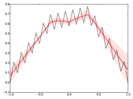
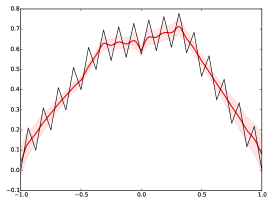
Figure 3: The average fit and standard deviation tubes for gradient descent and adadelta over 160,000 trials.

Figure 4 shows the absolute best fits over 160,000 trials each. Clearly, adadelta does better, but it can’t quite find an optimum.

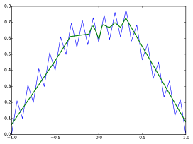
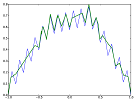
Figure 4: The best fits for gradient descent and adadelta over 160,000 trials.

4.4 Losses

The mean squared error loss corresponding to the average (smooth, low-frequency) fit is about $0.0045$. Figure 5 shows histograms of the losses over the 320,000 fits for both gradient descent and adadelta. Note the scales on the horizontal axes are quite small, so the qualitative difference between the distributions is exaggerated. Adadelta does better, but it has a wider variance, and both distributions have a large spike at the smooth fit. We do not have a good explanation for the specific features of either distribution, but it is clear that the barriers between the local and global minima are too high for either technique to climb over, and the energies associated with the individual local minima found by either technique are fairly similar.

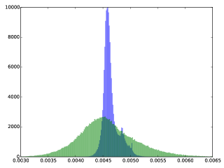
Figure 5: Histograms of the mean squared errors of gradient descent (blue) and adadelta (green) fits.

4.5 Distances between minima

We might ask: do we ever train to the same point? As discussed above, there are entire submanifolds of weight space which produce exactly the same output (so the set of local minima is not discrete), but we might hope that the symmetrization procedure from Section 3 would remove this issue, and after symmetrization we might find duplicate minima. In fact, we do not. Figure 6 shows histograms of the $L_{2}$ distances between $1,000,000$ randomly chosen pairs of trained weights. The minimum distances are both about $4$.

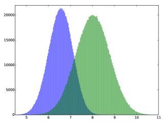
Figure 6: Histograms of the $L_{2}$ distances between pairs of weights of fitted models, with gradient descent (blue) and adadelta (green).

We can also compute the distances between a global minimum (the handcrafted weights, after symmetrization) and all the local minima. A histogram of these distances is shown in Figure 7.

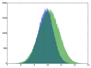
Figure 7: Histograms of the $L_{2}$ distances between the weights of fitted models and a global minimum, with gradient descent (blue) and adadelta (green).

It may seem somewhat paradoxical that all the pairs of local minima are within about distance 6-8 of each other, but they are also all about distance 10 from a global minimum. The only way for this to occur is if they are all to one side of the minimum, which seems counterintuitive. In fact, this is exactly the arrangement. Suppose we compute the direction vectors from the global minimum to each local minimum and take dot products of pairs of these vectors. If the local minima were distributed equally around the global minima, we would expect to find a range of dot products (including some negative ones). In fact, the minimum dot product is about $0.6$, indicating that the global minimum is off in a corner of the space. Note that this is not particularly surprising in high-dimensional space: a random Gaussian collection of points in $d$-dimensional space will have the same property, as long as there are fewer than exponentially (in $d$) many points.

4.6 NEB paths

Our goal is to gain some sense of the topography of the energy landscape. This is difficult, as the weight space has 136 dimensions. However, we can try to understand the landscape as we travel from a global minimum to a local minimum along a minimum energy path. This gives an idea of the terrain that the network must traverse under training if it is to find the global minimum. We used the nudged elastic band (NEB) method (see [6]) to find these minimal energy paths. These NEB paths demonstrate that the energy landscape is flat and slightly bumpy until a dramatic dropoff near the global minimum. See Figure 8. Such a landscape is extremely difficult for any gradient descent-based method to traverse.

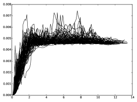
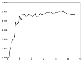
Figure 8: One hundred NEB paths from the global minimum to local minima (left), showing the very flat average terrain, and a single example NEB path (right). Note that in 136 dimensional weight space, the volume of the unit ball centered at the global minimum is much smaller than the volume of the shell of radius $9.5$ to $10.5$ which contains most of the local minima. The apparently gentle slope to the global minimum is an artifact of the one-dimensional NEB path and the chance of initializing the network to the domain of attraction of the global minimum is essentially $0$.

Although it is not particularly surprising, it is interesting to observe what happens to the output function as we travel along a NEB path. During the large, flat region of the path, the output changes very little as the function rearranges itself while preparing to create many spikes, which it does at the very end as it plunges towards the global minimum. See Figure 9.

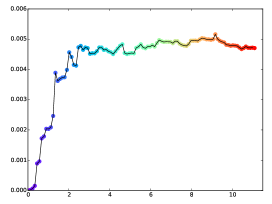
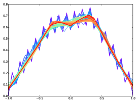
Figure 9: A single NEB path and the corresponding network output along the path.

Finally, we can get an idea of how complicated the energy function is near the global minimum by plotting the angles between successive difference vectors along a NEB path. Figure 10 gives an example of this.

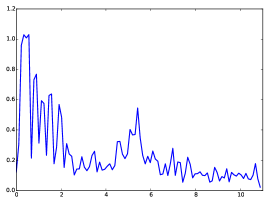
Figure 10: The angles (in radians) between successive difference vectors as we travel along the NEB path. The horizontal axis is distance along the path. Near the global minimum, the path twists and turns a lot.

As we expect, the path is required to do some twisting if it wants to approach the global minimum in an energy-minimizing way. We remark that we originally linearly interpolated between each pair of points along the NEB paths for plotting to increase their resolution, but we found that the interpolated points were useless: the energy function has such sharp curved valleys that the interpolated points have much larger loss.

4.7 Eigenvalues

To gain a further insight into the energy landscape near the minima, we can compute the eigenvalues of the Hessian of the loss. The use of the relu activation function means that the loss is not technically even $C^{1}$, but we expected that the single isolated issue at $0$ wouldn’t actually affect the computation of the Hessian. In fact, it does, and the numerical Hessian is neither symmetric nor stable. To avoid this issue, during the computation of the Hessian, we changed the activation function to $(1/5000)\log(1+\exp(5000x))$. This function, while smooth, is close enough to relu that the output of the network is not measurably changed. Figure 11 shows that at both kinds of minima, all eigenvalues are positive, and most of them are very small.

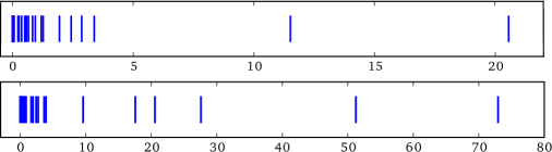
Figure 11: The eigenvalues of the Hessian of the loss function at local (top) and global (bottom) minima. Note there are 136 eigenvalues drawn; most of them are very close to $0$.

4.8 Basin of the global minimum

The obvious initial rise of the NEB paths gives us an indication of the size of the basin of attraction of the global minimum, but we can measure it another way: if we jitter the weights of the global minimum by a small amount and then retrain, we can find how much noise the model can take before it cannot find the global minimum again. Figure 12 shows the results of doing this experiment 4096 times with gradient descent and adadelta.

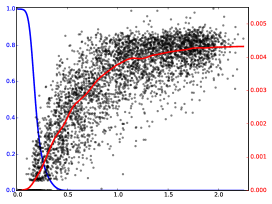
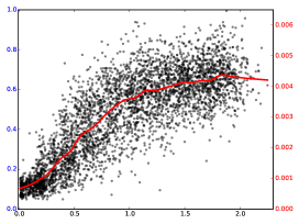
Figure 12: For both gradient descent and adadelta, a scatter plot of the final loss plotted as a function of the $L_{2}$ norm of the added noise (initial distance), and a lowess approximation (red). Also plotted is a logistic fit to the probability (blue) of returning to a global minimum as a function of the added noise amount. Note the two different vertical scales, and note that the probability curve for adadelta is not visible because it is identically zero.

For each experiment, we added a small amount of noise (with $L_{2}$ norm chosen approximately uniformly in $[0,2]$) and trained for 20,000 batches, just as with our main experiment above. We then compute the loss of the final model and plot it against the amount of noise added. It is strange that adadelta seems to never find a perfect fit. It is possible that it is doing small random walks, so stopping at a particular time is unlikely to yield an exact minimum. This agrees with our experience above.

4.9 Another example

Our main claim is that there are many functions which neural networks of a given size could reproduce perfectly but will never learn under training. Our main example is actually a very gentle one which does not even come close to the full complexity that a $5\times 5$ network can create. We now give some examples demonstrating this fact. See Figure 13.

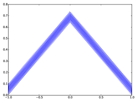
Figure 13: A $5\times(5+0)$ sawtooth (left); there are 3125 peaks and valleys, and a $5\times(3+2)$ model (right).

Obviously we expect to have trouble fitting such models with $5\times 5$ networks. Figure 14 shows an average fit plot analogous to Figure 3 and a NEB path between one of them and the global minimum.

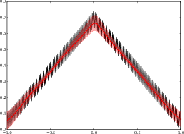
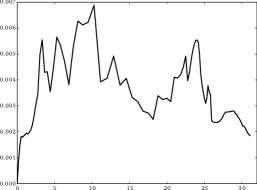
Figure 14: The average fit and standard deviation tube for 256 adadelta $5\times 5$ fits to the $5\times(3+2)$ model in Figure 13, and a NEB minimal energy path between the global minimum and one of these fits. Note the deviation in average fit plot is not due to some models fitting the function and some not: they all produce wiggle-free fits, but the exact location of the fitted function varies.

4.10 Larger networks

Let $W_{K,N}$ denote the weight space of $K\times N$ networks. Note that $W_{K,N}$ can be embedded in $W_{K^{\prime},N^{\prime}}$ for any $K^{\prime}\geq K$ and $N^{\prime}\geq N$ (and in many ways), so it is reasonable to ask how the topography of the weight space changes if we allow networks under training to move off the $W_{K,N}$ submanifold and through $W_{K^{\prime},N^{\prime}}$. That is, if we train a larger model. As we expect, this tends to turn local minima into saddle points and allow the network to learn more complex functions. For example, Figure 15 shows the first adadelta fit we did of a $10\times 10$ network to our main example function.

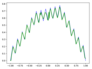
Figure 15: An adadelta $15\times 15$ fit to our main $5\times(2+3)$ example. It is evidently quite close to a global minimum.

5 Conclusion

We have shown (perhaps belabored) the point that the weight space of neural networks can be a complicated hilly place, and there can be global minima which are essentially unreachable using typical training techniques. The wide, flat local minima make optimization very difficult. In one sense, this is just the observation that nonconvex optimization is difficult. But this difficulty grants neural networks an interesting opportunity: because complex, high-frequency functions are difficult to fit, there is an implicit noise-dampening regularization built into the network, and training time becomes the parameter which controls how complex a the output of a network can be. So, in regression examples, at least, networks of moderate size will smooth rather than reproduce the training data.

In a perfect world, we might hope for a global-optimum oracle. In this case, we could obtain the same sort of regularization by limiting the effective size of our models. This is the standard approach in non-parametric regression, for example. Neural networks, on the other hand, with real-world optimization techniques appear to have the rather fortuitous property of being somewhat self-regularizing. How much we can rely on this fact remains a model selection problem.

References

- [1] Vijay Badrinarayanan, Bamdev Mishra, and Roberto Cipolla, Symmetry-invariant optimization in deep networks, arxiv:1511.01754
- [2] Andrew J. Ballard et. al., Perspective: energy landscapes for machine learning, preprint: arxiv:1703.07915
- [3] Kevin K. Chen The upper bound on knots in neural networks, preprint: arxiv:1611.09448
- [4] Kevin K. Chen, Anthony Gamst, and Alden Walker Knots in random neural networks, Workshop on Bayesian Deep Learning, NIPS 2016.
- [5] Kevin K. Chen, Anthony Gamst, and Alden Walker The empirical size of trained neural networks, preprint: arxiv:1611.09444
- [6] H. Jónsson, G. Mills, K. W. Jacobsen, Nudged elastic band method for finding minimum energy paths of transitions, Classical and Quantum Dynamics in Condensed Phase Simulations, Chapter 16, Ed. B. J. Berne, G. Ciccoti and D. F. Coker, 385 (World Scientific, 1998).