multicitedelim compcitedelim postnotedelim 297mm210mm* [] [] *32pc1.618 **1*** 2.5 *2* 2ex10mm0pt [nearest]   -1em0pt manaartplain manaart0.5 manaartPorta ManaMaximum-entropy from the probability calculus manaart0 plain0 plain manainitialplain manainitial0.5 manainitialPorta ManaMaximum-entropy from the probability calculus manaart0 mydate mydate figure   *  

Maximum-entropy from the probability calculus:
exchangeability, sufficiency

Dedicato alla mia fantastica sorellina Marianna per il suo compleanno

The classical maximum-entropy principle method [jaynes1963] appears in the probability calculus as an approximation of a particular model by exchangeability or a particular model by sufficiency.

The approximation from the exchangeability model can be inferred from an analysis by Jaynes *jaynes1986d_r1996 and to some extent from works on entropic priors [rodriguez1989, rodriguez2002, skilling1989b, skilling1990]. I tried to show it explicitly in a simple context [portamana2009]. The approximation from the sufficiency model can be inferred from Bernardo & Smith *[§ 4.5]bernardoetal1994_r2000 and Diaconis & Freedman *diaconisetal1981 in combination with the Koopman-Pitman-Darmois theorem see references in § 3.

In this note I illustrate how either approximations arises, in turn, and then give a heuristic synopsis of both. At the end I discuss some questions: Prediction or retrodiction? Which of the two models is preferable? (the exchangeable one.) How good is the maximum-entropy approximation? Is this a “derivation” of maximum-entropy?

I assume that you are familiar with: the maximum-(relative-)entropy method jaynes1957[much clearer in][]jaynes1963sivia1996_r2006,hobsonetal1973, especially the mathematical form of its distributions and its prescription “expectations = empirical averages”; the probability calculus [jaynes1994_r2003, hailperin1996, jeffreys1939_r2003, lindley2006_r2014]; the basics of models by exchangeability and sufficiency [bernardoetal1994_r2000, ch. 4], although I’ll try to explain the basic ideas behind them – likely you’ve often worked with them even if you’ve never heard of them under these names.

1 Context and notation

We have a potentially infinite set of measurements, each having $K$ possible outcomes. Dice rolls and their six outcomes are a typical example. I use the terms “measurement” and “outcome” to lend concreteness to the discussion, but the formulae below apply to much more general contexts.

The proposition that the $n$th measurement has outcome $k$ is denoted ${}^{(n)}_{k}$. The relative frequencies of the $K$ possible outcomes in a set of measurements are denoted $\bm{f}\coloneqq(f_{k})$. It may happen that in a measurement we observe not directly an outcome but an “observable” having values $(O_{k})\eqqcolon\bm{O}$ for the $K$ outcomes. This observable may be vector-valued. The empirical average of the observable in a set of $N$ measurements with outcomes $\{k_{1},\dotsc,k_{N}\}$ is $\sumop\slimits@_{n=1}^{N}O_{k_{n}}/N$, equivalent to $\sumop\slimits@_{k}O_{k}f_{k}$.

Probabilities have propositions as arguments (for good definitions of what a proposition is – it isn’t a sentence, for example – see)()strawson1952_r1964,copi1954_r1979,barwiseetal1999_r2003. Johnson’s definition remains one of the simplest and most beautiful: “Probability is a magnitude to be attached to any possibly true or possibly false proposition; not, however, to the proposition in and for itself, but in reference to another proposition the truth of which is supposed to be known” [johnson1924, Appendix, § 2]. See also Hailperin’s *hailperin1996,hailperin2011 formalization, sadly neglected in the literature. The assumptions or knowledge underlying our probabilities – our “model” – will be generically denoted by , with subscripts denoting specific assumptions. We will sometimes let a quantity stand as abbreviation for a proposition, for example $\bm{f}$ for “the observed relative frequencies in $N$ measurements are $\bm{f}$”. In such cases the probability symbol will be in lower-case to remind us of our notational sins.

Lest this note become an anthill of indices let’s use the following notation: for positive $K$-tuples $\bm{x}\coloneqq(x_{i})$, $\bm{y}\coloneqq(y_{i})$, and number $a$,

$$\begin{gathered}a\bm{x}\coloneqq(ax_{i}),\qquad\bm{x}/\bm{y}\coloneqq(x_{i}/y_{i}),\qquad\bm{x}\bm{y}\coloneqq(x_{i}y_{i}),\qquad\bm{x}^{\bm{y}}\coloneqq({x_{i}}^{y_{i}}),\\ \exp\bm{x}\coloneqq(\exp x_{i}),\qquad\ln\bm{x}\coloneqq(\ln x_{i}),\qquad\bm{x}!\coloneqq(x_{i}!),\\ \mathop{\textstyle\sumop\slimits@}\nolimits\bm{x}\coloneqq\sumop\slimits@_{k}x_{k},\qquad\mathop{\textstyle\prodop\slimits@}\nolimits\bm{x}\coloneqq\prodop\slimits@_{k}x_{k},\qquad\binom{a}{a\bm{x}}\coloneqq\frac{a!}{\mathop{\textstyle\prodop\slimits@}\nolimits(a\bm{x})!}.\end{gathered}$$ (1)

The symbol indicates a Dirac delta [lighthill1958_r1964][even better:][]egorov1990,egorov2001 or a characteristic function [knuth1992, cf.], depending on the context.

The Shannon entropy $H(\bm{x})\coloneqq-\mathop{\textstyle\sumop\slimits@}\nolimits\bm{x}\ln\bm{x}$, and the relative Shannon entropy or negative discrimination information $H(\bm{x};\bm{y})\coloneqq-\mathop{\textstyle\sumop\slimits@}\nolimits\bm{x}\ln(\bm{x}/\bm{y})$. Let’s keep in mind the important properties

$$H(\bm{x};\bm{y})\leqslant 0,\qquad H(\bm{x};\bm{y})=0\Leftrightarrow\bm{x}=\bm{y}.$$ (2)

The problem typically addressed by maximum-entropy is this: given that in a large number $N$ of measurements we have observed an average having value in a convex set $A$ (which can consist of a single number),

$$\mathop{\textstyle\sumop\slimits@}\nolimits\bm{O}\bm{f}\in A,$$ (3)

what is the probability of having outcome $k$ in an $(N+1)$th measurement? In symbols,

$$\mathrm{P}\bigl{[}{}^{(N+1)}_{k}\mathpunct{\big{|}\ }\mathop{\textstyle\sumop\slimits@}\nolimits\bm{O}\bm{f}\in A,\varIota\bigr{]}=\mathord{?}$$ (4)

where denotes our state of knowledge. The maximum-entropy answer [meadetal1984, fangetal1997, boydetal2004_r2009] has the form

$$\frac{r_{k}\exp(\lambda O_{k})}{\sumop\slimits@\bm{r}\exp(\lambda\bm{O})}$$ (5)

where $\bm{r}$ is a reference distribution and is determined by the constraints in a way that we don’t need to specify here. The convexity of $A$ ensures the uniqueness of this answer.

2 Maximum-entropy from a model by exchangeability

Let’s assume that in our state of knowledge ${}_{\text{x}}$ we deem the measurements to be infinitely exchangeable [bernardoetal1994_r2000, § 4.2]; that is, there can be a potentially unlimited number of them and their indices are irrelevant for our inferences. De Finetti’s theorem [*]definetti1930,definetti1937; [heathetal1976] states that this assumption forces us to assign probabilities of this form:

$$\mathrm{P}\bigl{[}{}^{(1)}_{k_{1}},\dotsc,{}^{(N)}_{k_{N}}\mathpunct{\big{|}\ }{}_{\text{x}}\bigr{]} =\int q_{k_{1}}\dotsm q_{k_{N}}\,\mathrm{p}(\bm{q}\mathpunct{|}{}_{\text{x}})\,\mathrm{d}\bm{q}$$ (6)

$$\equiv\int\Bigl{(}\mathop{\textstyle\prodop\slimits@}\nolimits\bm{q}^{N\bm{f}}\Bigr{)}\,\mathrm{p}(\bm{q}\mathpunct{|}{}_{\text{x}})\,\mathrm{d}\bm{q},$$

where the distribution $\bm{q}$ can be interpreted as the relative frequencies in the long run, and integration is over the $(K-1)$-dimensional simplex [gruenbaum1967_r2003] of such distributions, $\{\bm{q}\in\bm{\mathrm{R}}_{\geqslant 0}^{K}\mid\mathop{\textstyle\sumop\slimits@}\nolimits\bm{q}=1\}$. The term $\mathrm{p}(\bm{q}\mathpunct{|}{}_{\text{x}})\,\mathrm{d}\bm{q}$ can be interpreted as the prior probability density of observing the long-run frequencies $\bm{q}$ in an infinite number of measurements. This probability is not determined by the theorem.

Let’s call the expression above an exchangeability model [bernardoetal1994_r2000, § 4.3].

We assume that our state of knowledge ${}_{\text{x}}$ is also expressed by a particular prior density for the long-run frequencies:

$$\mathrm{p}(\bm{q}\mathpunct{|}{}_{\text{x}})\,\mathrm{d}\bm{q}=\kappa(L,\bm{r})\,\binom{L}{L\bm{q}}\,\mathop{\textstyle\prodop\slimits@}\nolimits\bm{r}^{L\bm{q}}\,\mathrm{d}\bm{q},\qquad L\geqslant 1,$$ (7)

which we can call “multinomial prior” because is a sort of continuous interpolation of the multinomial distribution [johnsonetal1969_r1996, ch. 35]. in the latter each $q_{k}$ assumes discrete values in $\{0,1/L,\dotsc,1\}$ and the normalizing constant is unity; for this reason the normalizing constant $\kappa(L,\bm{r})\approx L$ in eq. (7). The results that follow also hold for any other prior density that is asymptotically equal to the one above for $L$ large, for example proportional to $\exp[LH(\bm{q};\bm{r})]$, which appears in Rodríguez’s *rodriguez1989,rodriguez2002 entropic prior and in Skilling’s *skilling1989b,skilling1990 prior for “classical” and “quantified” maximum-entropy.

To find the probability (4) queried by maximum-entropy we need the probability for each possible frequency distribution in the $N$ measurements, which by combinatorial arguments is

$$\mathrm{p}(\bm{f}\mathpunct{|}{}_{\text{x}})=\int\binom{N}{N\bm{f}}\,\Bigl{(}\mathop{\textstyle\prodop\slimits@}\nolimits\bm{q}^{N\bm{f}}\Bigr{)}\,\mathrm{p}(\bm{q}\mathpunct{|}{}_{\text{x}})\,\mathrm{d}\bm{q}.$$ (8)

There are $\binom{N+K-1}{K-1}$ possible frequency distributions [csiszaretal2004b].

By marginalization over the subset of frequencies consistent with our data, the probability for the empirical average is

$$\mathrm{P}\bigl{(}\mathop{\textstyle\sumop\slimits@}\nolimits\bm{O}\bm{f}\in A\mathpunct{\big{|}\ }{}_{\text{x}}\bigr{)}=\sumop\slimits@_{\bm{f}}\deltaup(\mathop{\textstyle\sumop\slimits@}\nolimits\bm{O}\bm{f}\in A)\int\binom{N}{N\bm{f}}\,\Bigl{(}\mathop{\textstyle\prodop\slimits@}\nolimits\bm{q}^{N\bm{f}}\Bigr{)}\,\mathrm{p}(\bm{q}\mathpunct{|}{}_{\text{x}})\,\mathrm{d}\bm{q}.$$ (9)

Finally using Bayes’s theorem with the probabilities (6)–(9) we find

$$\mathrm{P}\bigl{[}{}^{(N+1)}_{k}\mathpunct{\big{|}\ }\mathop{\textstyle\sumop\slimits@}\nolimits\bm{O}\bm{f}\in A,{}_{\text{x}}\bigr{]}=\frac{\int q_{k}\sumop\slimits@_{\bm{f}}\deltaup(\mathop{\textstyle\sumop\slimits@}\nolimits\bm{O}\bm{f}\in A)\,\binom{N}{N\bm{f}}\,\bigl{(}\mathop{\textstyle\prodop\slimits@}\nolimits\bm{q}^{N\bm{f}}\bigr{)}\,\mathrm{p}(\bm{q}\mathpunct{|}{}_{\text{x}})\,\mathrm{d}\bm{q}}{\int\sumop\slimits@_{\bm{f}}\deltaup(\mathop{\textstyle\sumop\slimits@}\nolimits\bm{O}\bm{f}\in A)\,\binom{N}{N\bm{f}}\,\bigl{(}\mathop{\textstyle\prodop\slimits@}\nolimits\bm{q}^{N\bm{f}}\bigr{)}\,\mathrm{p}(\bm{q}\mathpunct{|}{}_{\text{x}})\,\mathrm{d}\bm{q}},$$ (10)

where the density $\mathrm{p}(\bm{q}\mathpunct{|}{}_{\text{x}})\,\mathrm{d}\bm{q}$ is specified in eq. (7), even though the formula above holds as well with any other prior density.

I have graphically emphasized this formula because it is the exact answer given to the question (4) by a general exchangeability model: it holds for all numbers $K$ of possible outcomes, all numbers $N$ of observations, and all sets $A$ – even non-convex ones.

If $N$ and $L$ are large we can use the bounds of the multinomial [csiszaretal1981, Lemma 2.3]

$$\binom{N}{N\bm{f}}=\epsilon(N,\bm{f})\exp[N\,H(\bm{f})],\quad(N+1)^{-K}\leqslant\epsilon(N,\bm{f})\leqslant 1,$$ (11)

analogously for $\binom{L}{L\bm{r}}$.

From the bounds above it can be shown that the exact probability expression (10) has the asymptotic form

$$\mathrm{P}\bigl{[}{}^{(N+1)}_{k}\mathpunct{\big{|}\ }\mathop{\textstyle\sumop\slimits@}\nolimits\bm{O}\bm{f}\in A,{}_{\text{x}}\bigr{]}\simeq{}\\ \kappa(N,L,\bm{r})\int q_{k}\sumop\slimits@_{\bm{f}}\deltaup(\mathop{\textstyle\sumop\slimits@}\nolimits\bm{O}\bm{f}\in A)\,\exp[NH(\bm{f};\bm{q})+LH(\bm{q};\bm{r})]\,\mathrm{d}\bm{q},\\ \text{$N$, $L$ large}.$$ (12)

I prefer the symbol “$\simeq$”, “is asymptotically equal to” [iso1993_r2009, ieee1993, iupac1988_r2007], to the limit symbol “$\to$” because the latter may invite to think about a sequence, but no such sequence exists. In each specific problem $N$ has one, fixed, possibly unknown value, and cannot be increased at will. The symbol “$\simeq$” says that the right side differs from the left side by an error that may be negligible. It is our duty to check whether this error is really negligible for our purposes.

The asymptotic expression above shows an interesting interplay of two relative entropies. The two exponential terms give rise to two Dirac deltas. The delta in $\bm{f}$ requires some mathematical care owing to the discreteness of this quantity; see Csiszár *csiszar1984,csiszar1985. In particular, if $N<K$ the discrete set of $\binom{N+K-1}{K-1}$ possible frequency distributions lies within the $(N-1)$-dimensional facets of the $(K-1)$-dimensional simplex of distributions $\bm{q}$; it does not “fill” the simplex. In this case the frequency sum $\sumop\slimits@_{\bm{f}}$ cannot be meaningfully approximated by an integral. The approximations below are valid if the number $N$ of observations is much larger than the number $K$ of possible outcomes.

If $L/N$ is also large, taking limits in the proper order gives

$$\mathrm{P}\bigl{[}{}^{(N+1)}_{k}\mathpunct{\big{|}\ }\mathop{\textstyle\sumop\slimits@}\nolimits\bm{O}\bm{f}\in A,{}_{\text{x}}\bigr{]}\simeq r_{k},\qquad\text{$N$, $L$, $L/N$ large}.$$ (13)

Note how the data about the average (3) are practically discarded in this $(L/N)$-large case. Compare with Skilling’s remark that the parameter $L$ (his ) shouldn’t be “particularly large” [skilling1998, cf.].

The asymptotic case that interests us is $N/L$ large: the exponential in $N$ dominates the integral of eq. (12), which becomes

$$\kappa(L,\bm{r})\sumop\slimits@_{\bm{f}}\bm{f}_{k}\,\deltaup[\mathop{\textstyle\sumop\slimits@}\nolimits\bm{O}\bm{f}\in A]\,\exp[LH(\bm{f};\bm{r})]\simeq\operatorname*{arg\,sup}\limits_{\bm{f}}^{\sumop\slimits@\bm{O}\bm{f}\in A}H(\bm{f};\bm{r}),$$ (14)

so that, finally,

$$\mathrm{P}\bigl{[}{}^{(N+1)}_{k}\mathpunct{\big{|}\ }\mathop{\textstyle\sumop\slimits@}\nolimits\bm{O}\bm{f}\in A,{}_{\text{x}}\bigr{]}\simeq f^{*}_{k},\qquad\text{$N$, $L$, $L/N$ large},\\ \text{with $\bm{f}^{*}$ maximizing $H(\bm{f};\bm{r})$ under constraints $\mathop{\textstyle\sumop\slimits@}\nolimits\bm{O}\bm{f}\in A$},$$ (15)

which is the maximum-entropy recipe, giving the distribution (5).

3 Maximum-entropy from a model by sufficiency

Consider the following assumption or working hypothesis, denoted ${}_{\text{s}}$: To predict the outcome of an $(N+1)$th measurement given knowledge of the outcomes of $N$ measurements, all we need to know is the average $\mathop{\textstyle\sumop\slimits@}\nolimits\bm{O}\bm{f}$ of an observable $\bm{O}$ in those $N$ measurements, no matter the value of $N$. In other words, any data about known measurements, besides the empirical average of $\bm{O}$, is irrelevant for our prediction. The average $\mathop{\textstyle\sumop\slimits@}\nolimits\bm{O}\bm{f}$ is then called a minimal sufficient statistics [bernardoetal1994_r2000, § 4.5][§ 5.5]lindley1965b_r2008. In symbols,

$$\mathrm{P}\bigl{[}{}^{(N+1)}_{k}\mathpunct{\big{|}\ }{}^{(1)}_{k_{1}},\dotsc,{}^{(N)}_{k_{N}},{}_{\text{s}}\bigr{]}=\mathrm{p}\bigl{[}{}^{(N+1)}_{k}\mathpunct{\big{|}\ }\mathop{\textstyle\sumop\slimits@}\nolimits\bm{O}\bm{f},N,{}_{\text{s}}\bigr{]}.$$ (16)

Note that the data $\{{}^{(n)}_{k_{n}}\}$ determine the data $\{\mathop{\textstyle\sumop\slimits@}\nolimits\bm{O}\bm{f},N\}$ but not vice versa, so some data have effectively been discarded in the conditional.

The Koopman-Pitman-Darmois theorem [koopman1936, pitman1936, darmois1935][see also later analyses:][]hipp1974,andersen1970,denny1967,fraser1963,barankinetal1963 states that this assumption forces us to assign probabilities of this form:

$$\!\begin{aligned} \mathrm{P}\bigl{[}{}^{(1)}_{k_{1}},\dotsc,{}^{(N)}_{k_{N}}\mathpunct{\big{|}\ }{}_{\text{s}}\bigr{]}&=\int\mathrm{p}(k_{1}\mathpunct{|}\lambda,\bm{r},{}_{\text{s}})\dotsm\mathrm{p}(k_{N}\mathpunct{|}\lambda,\bm{r},{}_{\text{s}})\,\mathrm{p}(\lambda\mathpunct{|}{}_{\text{s}})\,\mathrm{d}\lambda,\\[3.0pt] &\equiv\int\Bigl{[}\mathop{\textstyle\prodop\slimits@}\nolimits\mathrm{p}(\bm{k}\mathpunct{|}\lambda,\bm{r},{}_{\text{s}})^{N\bm{f}}\Bigr{]}\,\mathrm{p}(\lambda\mathpunct{|}{}_{\text{s}})\,\mathrm{d}\lambda,\end{aligned}$$ (17a)

$$\text{with}\quad\mathrm{p}(\bm{k}\mathpunct{|}\lambda,\bm{r},{}_{\text{s}})\coloneqq\bm{r}\frac{\exp(\lambda\bm{O})}{Z(\lambda)},\quad Z(\lambda)\coloneqq\mathop{\textstyle\sumop\slimits@}\nolimits\bm{r}\exp(\lambda\bm{O}),$$ (17b)

and we have defined $\mathrm{p}(\bm{k}\mathpunct{|}\dotso)\coloneqq\bigl{(}\mathrm{p}(1\mathpunct{|}\dotso),\dotsc,\mathrm{p}(K\mathpunct{|}\dotso)\bigr{)}$. The integration of the parameter is over $\bm{\mathrm{R}}^{M}$, with $M$ the dimension of the vector-valued observable $\bm{O}$, and $\bm{r}$ is a $K$-dimensional distribution. Neither $\bm{r}$ or the distribution $\mathrm{p}(\lambda\mathpunct{|}{}_{\text{s}})$ are determined by the theorem.

Let’s call the expression above a sufficiency model [bernardoetal1994_r2000, § 4.5]. A sufficiency model can be viewed as a mixture, with weight density $\mathrm{p}(\lambda\mathpunct{|}{}_{\text{s}})\,\mathrm{d}\lambda$, of distributions having maximum-entropy form (5) with multipliers .

To find the probability (4) we calculate, as in the previous section, the probabilities for the frequencies:

$$\mathrm{p}(\bm{f}\mathpunct{|}{}_{\text{s}})=\int\binom{N}{N\bm{f}}\,\Bigl{[}\mathop{\textstyle\prodop\slimits@}\nolimits\mathrm{p}(\bm{k}\mathpunct{|}\lambda,\bm{r},{}_{\text{s}})^{N\bm{f}}\Bigr{]}\,\mathrm{p}(\lambda\mathpunct{|}{}_{\text{s}})\,\mathrm{d}\lambda,$$ (18)

and for the empirical average by marginalization:

$$\mathrm{P}\bigl{(}\mathop{\textstyle\sumop\slimits@}\nolimits\bm{O}\bm{f}\in A\mathpunct{\big{|}\ }{}_{\text{s}}\bigr{)}={}\\ \sumop\slimits@_{\bm{f}}\deltaup(\mathop{\textstyle\sumop\slimits@}\nolimits\bm{O}\bm{f}\in A)\int\binom{N}{N\bm{f}}\,\Bigl{[}\mathop{\textstyle\prodop\slimits@}\nolimits\mathrm{p}(\bm{k}\mathpunct{|}\lambda,\bm{r},{}_{\text{s}})^{N\bm{f}}\Bigr{]}\,\mathrm{p}(\lambda\mathpunct{|}{}_{\text{s}})\,\mathrm{d}\lambda.$$ (19)

From these using Bayes’s theorem we finally find

$$\mathrm{P}\bigl{[}{}^{(N+1)}_{k}\mathpunct{\big{|}\ }\mathop{\textstyle\sumop\slimits@}\nolimits\bm{O}\bm{f}\in A,{}_{\text{s}}\bigr{]}={}\\[9.0pt] \frac{\int\mathrm{p}(k\mathpunct{|}\lambda,\bm{r},{}_{\text{s}})\sumop\slimits@_{\bm{f}}\deltaup(\mathop{\textstyle\sumop\slimits@}\nolimits\bm{O}\bm{f}\in A)\,\binom{N}{N\bm{f}}\,\bigl{[}\mathop{\textstyle\prodop\slimits@}\nolimits\mathrm{p}(\bm{k}\mathpunct{|}\lambda,\bm{r},{}_{\text{s}})^{N\bm{f}}\bigr{]}\,\mathrm{p}(\lambda\mathpunct{|}{}_{\text{s}})\,\mathrm{d}\lambda}{\int\sumop\slimits@_{\bm{f}}\deltaup(\mathop{\textstyle\sumop\slimits@}\nolimits\bm{O}\bm{f}\in A)\,\binom{N}{N\bm{f}}\,\bigl{[}\mathop{\textstyle\prodop\slimits@}\nolimits\mathrm{p}(\bm{k}\mathpunct{|}\lambda,\bm{r},{}_{\text{s}})^{N\bm{f}}\bigr{]}\,\mathrm{p}(\lambda\mathpunct{|}{}_{\text{s}})\,\mathrm{d}\lambda}.$$ (20)

This is the exact answer given to the maximum-entropy question by a sufficiency model if the constraints used in maximum-entropy are considered to be a sufficient statistics. This proviso has serious consequences discussed in § 5.2. The expression above holds for all $N$ and all sets $A$, even non-convex ones.

The asymptotic analysis for large $N$ uses again the multinomial’s bounds (11). We find

$$\mathrm{P}\bigl{[}{}^{(N+1)}_{k}\mathpunct{\big{|}\ }\mathop{\textstyle\sumop\slimits@}\nolimits\bm{O}\bm{f}\in A,{}_{\text{s}}\bigr{]}\simeq\kappa(N,\bm{r})\int\mathrm{p}(k\mathpunct{|}\lambda,\bm{r},{}_{\text{s}})\times{}\\ \sumop\slimits@_{\bm{f}}\deltaup(\mathop{\textstyle\sumop\slimits@}\nolimits\bm{O}\bm{f}\in A)\,\exp\bigl{\{}NH\bigl{[}\bm{f};\mathrm{p}(\bm{k}\mathpunct{|}\lambda,\bm{r},{}_{\text{s}})\bigr{]}\bigr{\}}\,\mathrm{p}(\lambda\mathpunct{|}{}_{\text{s}})\,\mathrm{d}\lambda,\\[-10.00002pt] \text{$N$ large}.$$ (21)

A rigorous analysis of this limit can be done using “information projections” [csiszar1984, csiszar1985]; here is a heuristic summary. Consider the sum in $\bm{f}$ for fixed . We have two cases. (1) If is such that $\mathop{\textstyle\sumop\slimits@}\nolimits\bm{O}\,\mathrm{p}(\bm{k}\mathpunct{|}\lambda,\bm{r},{}_{\text{s}})\in A$, there exists a unique $\bm{f}$ in the sum for which the relative entropy in the exponential reaches its maximum, zero, making the exponential unity. For all other $\bm{f}$ the relative entropy is negative and the exponential asymptotically vanishes for large $N$ . The integral therefore doesn’t vanish asymptotically. (2) If is such that $\mathrm{p}(\bm{k}\mathpunct{|}\lambda,\bm{r},{}_{\text{s}})$ doesn’t satisfy the constraints, the relative entropy in the exponential will be negative for all $\bm{f}$ in the sum, making the exponential asymptotically vanish for all $\bm{f}$. The integral therefore vanishes asymptotically. The distinction between these two cases actually requires mathematical care owing to the discreteness of the sum. The $\bm{f}$ sum then acts as a delta or characteristic function (depending on whether $A$ has measure zero or not):

$$\sumop\slimits@_{\bm{f}}\deltaup(\mathop{\textstyle\sumop\slimits@}\nolimits\bm{O}\bm{f}\in A)\,\exp\bigl{\{}NH\bigl{[}\bm{f};\mathrm{p}(\bm{k}\mathpunct{|}\lambda,\bm{r},{}_{\text{s}})\bigr{]}\bigr{\}}\simeq\deltaup\bigl{[}\mathop{\textstyle\sumop\slimits@}\nolimits\bm{O}\,\mathrm{p}(\bm{k}\mathpunct{|}\lambda,\bm{r},{}_{\text{s}})\in A\bigr{]}.$$ (22)

Thus asymptotically we have, using the explicit expression (17b) for $\mathrm{p}(\bm{k}\mathpunct{|}\lambda,\bm{r},{}_{\text{s}})$:

$$\mathrm{P}\bigl{[}{}^{(N+1)}_{k}\mathpunct{\big{|}\ }\mathop{\textstyle\sumop\slimits@}\nolimits\bm{O}\bm{f}\in A,{}_{\text{s}}\bigr{]}\simeq{}\\ \int\deltaup\biggl{[}\mathop{\textstyle\sumop\slimits@}\nolimits\bm{O}\,\bm{r}\frac{\exp(\lambda\bm{O})}{Z(\lambda)}\in A\biggr{]}\,r_{k}\frac{\exp(\lambda O_{k})}{Z(\lambda)}\,\mathrm{p}(\lambda\mathpunct{|}{}_{\text{s}})\,\mathrm{d}\lambda,\quad\text{$N$ large}.$$ (23)

This result can also be found first integrating and then summing $\bm{f}$, using a heuristic argument similar to the one above. This is a mixture, with weight density $\mathrm{p}(\lambda\mathpunct{|}{}_{\text{s}})\,\mathrm{d}\lambda$, of maximum-relative-entropy distributions $\bm{f}^{*}$ that satisfy the individual constraints $\mathop{\textstyle\sumop\slimits@}\nolimits\bm{O}\bm{f}^{*}=a$, $a\in A$ . The final distribution thus differs from the maximum-entropy one if the set $A$ is not a singleton: maximum-entropy would pick up only one distribution. But if the constraint set is a singleton, $A=\{a\}$, we do obtain the same answer (5) as the maximum-entropy recipe:

$$\mathrm{P}\bigl{[}{}^{(N+1)}_{k}\mathpunct{\big{|}\ }\mathop{\textstyle\sumop\slimits@}\nolimits\bm{O}\bm{f}=a,{}_{\text{x}}\bigr{]}\simeq f^{*}_{k},\qquad\text{$N$ large},\\ \text{with $\bm{f}^{*}$ maximizing $H(\bm{f};\bm{r})$ under constraints $\mathop{\textstyle\sumop\slimits@}\nolimits\bm{O}\bm{f}=a$}.$$ (24)

4 Heuristic explanation of both asymptotic approximations

First of all let’s note that both the exchangeability (6) and sufficiency (17) models have the parametric form

$$\mathrm{P}\bigl{[}{}^{(1)}_{k_{1}},\dotsc,{}^{(N)}_{k_{N}}\mathpunct{\big{|}\ }\varIota\bigr{]} =\int\mathrm{p}(k_{1}\mathpunct{|}\nu,\varIota)\dotsm\mathrm{p}(k_{N}\mathpunct{|}\nu,\varIota)\,\mathrm{p}(\nu\mathpunct{|}\varIota)\,\mathrm{d}\nu$$ (25)

$$\equiv\int\Bigl{[}\mathop{\textstyle\prodop\slimits@}\nolimits\mathrm{p}(\bm{k}\mathpunct{|}\nu,\varIota)^{N\bm{f}}\Bigr{]}\,\mathrm{p}(\nu\mathpunct{|}\varIota)\,\mathrm{d}\nu.$$

The final probability distribution $\bm{p}$ for the $K$ outcomes of the $(N+1)$th measurement belongs to a $(K-1)$-dimensional simplex $\{\bm{p}\in\bm{\mathrm{R}}_{\geqslant 0}^{K}\mid\mathop{\textstyle\sumop\slimits@}\nolimits\bm{p}=1\}$. The expression above first selects, within this simplex, a family of distributions $\{\mathrm{p}(\bm{k}\mathpunct{|}\nu,\varIota)\}$ parametrized by ; then it delivers the distribution $\bm{p}$ as a mixture of the distributions of this family, with weight density $\mathrm{p}(\nu\mathpunct{|}\varIota)\,\mathrm{d}\nu$. In the exchangeability model this family is actually the whole simplex (that’s why it’s sometimes called a “non-parametric” model). In the sufficiency model it is an exponential family [bernardoetal1994_r2000, § 4.5.3]barndorffnielsen1978_r2014.

When we conditionalize on data $D$, the weight density is determined by the mutual modulation of two weights: that of the probability of the data $\mathrm{p}(D\mathpunct{|}\nu,\varIota)$ and the initial weight $\mathrm{p}(\nu\mathpunct{|}\varIota)$. Pictorially, if $K=3$:

$$\begin{gathered}\makebox{\includegraphics[width=390.25534pt]{conf50050new.png}}\\ \makebox[91.0631pt][l]{$\mathrm{p}(D\mathpunct{|}\nu,\varIota)$}\times\makebox[121.41306pt][c]{$\mathrm{p}(\nu\mathpunct{|}\varIota)$}=\makebox[91.0631pt][r]{$\kappa\mathrm{p}(\nu\mathpunct{|}D,\varIota)$}\end{gathered}$$ (26)

the final $\bm{p}$ is given by the mixture with the weight density $\mathrm{p}(\nu\mathpunct{|}D,\varIota)\,\mathrm{d}\nu$ ensuing from this modulation. The mathematical expression of the data weight $\mathrm{p}(D\mathpunct{|}\nu,\varIota)$ is typically exponentiated to the number of measurements $N$ from which the data originate; compare with eqs (19), (20). If $N$ is large this weight is very peaked on the subset of distributions that give highest probability to the data, that is, that have expectations very close to the empirical averages. It effectively restricts the second weight $\mathrm{p}(\nu\mathpunct{|}\varIota)\,\mathrm{d}\nu$ to such “data subset”. In our case the data subset consists of all distributions satisfying the constraints.

The mechanism described so far is common to the exchangeability and the sufficiency model. Their difference lies in how they choose the final distribution from the data subset.

In the exchangeability model (6) the choice is made by the weight density $\mathrm{p}(\nu\mathpunct{|}\varIota)\,\mathrm{d}\nu$, i.e. the multinomial prior (7). It is extremely peaked owing to the large parameter $L$, and its level curves are isentropics. Once it’s restricted to the data subset by the data weight $\mathrm{p}(D\mathpunct{|}\nu,\varIota)$, it gives highest weight to the distribution $\bm{p}$ lying on the highest isentropic curve, which is unique if the data subset is convex; compare with fig.-eq. (26). Hence this is a maximum-entropy distribution satisfying the data constraints. For this mechanism to work it’s necessary that the dominance of the data weight comes first, and the dominance of the multinomial prior comes second. This is the reason why the correct asymptotic limit (15) has $N$, $L$, and $N/L$ large.

In the sufficiency model (17) the choice is made by the family of distributions $\{\mathrm{p}(\bm{k}\mathpunct{|}\nu,\varIota)\}$. These distributions have by construction a maximum-entropy form for the particular observable $\bm{O}$. This family intersects the data subset in only one point if the constraint has the form $\mathop{\textstyle\sumop\slimits@}\nolimits\bm{O}\bm{f}=a$. This point is therefore the maximum-entropy distribution satisfying the data constraints.

The mechanism above also explains why these two models still work if the data subset is non-convex and touches the highest isentropics (exchangeability model) or the exponential family (sufficiency model) in multiple points, bringing the maximum-entropy recipe to an impasse. The final distribution will simply be an equal mixture of such tangency points; it may well lie outside of the data subset.

5 Discussion

5.1 Prediction or retrodiction?

An essential aspect of the maximum-entropy method is surprisingly often disregarded in the literature. If we have data from $N$ measurements, we can ask two questions:

“Prediction”:

what is the outcome of a further similar measurement?

“Retrodiction”:

what is the outcome of the first of the $N$ measurements?

Note that despite the literal meaning of these terms the distinction is not between future and past, but between unknown and partially known.

It’s rarely made clear whether the maximum-entropy probabilities refer to the first or to the second question. Yet these two questions are fundamentally different; their answers rely on very different principles.

To answer the first question we can – but need not – fully rely on symmetry principles in the discrete case. It is a matter of combinatorics and equal probabilities; a drawing-from-an-urn problem. Most derivations of the maximum-entropy method [jaynes1963, shoreetal1980, vancampenhoutetal1981, csiszar1985, e.g.] address this question only, as often betrayed by the presence of “$p(x_{1})$” or similar expressions in their final formulae.

To answer the second question, symmetry and combinatorics alone are no use: additional principles are needed. This is the profound philosophical question of induction, with its ocean of literature; my favourite sample are the classic Hume *[book I, § III.VI]hume1739_r1896, Johnson *[esp. chs VIII ff]johnson1922[Appendix]johnson1924johnson1932c, de Finetti *definetti1937,definetti1959b, Jeffreys *jeffreys1955[ch. I]jeffreys1931_r1973[§ 1.0]jeffreys1939_r2003, Jaynes *[§ 9.4]jaynes1994_r2003. De Finetti, foreshadowed by Johnson, was probably the one who expressed most strongly, and explained brilliantly, that the probability calculus does not and cannot explain or justify our inductive reasoning; it only expresses it in a quantitative way. This shift in perspective was very much like Galilei’s shift from why to how in the study of physical phenomena. We do inductive inferences in many different ways [jaynes1994_r2003, § 9.4]. The notion of exchangeability [definetti1937][Appendix]johnson1924johnson1932c captures one of the most intuitive and expresses it mathematically.

The calculations of the previous sections and the final probabilities (10), (20) for our two models pertain the predictive question, as clear from the ^(N+1) in their arguments. The two models can also be used to answer the retrodictive question. The resulting formulae are different; they can again be found applying the rules of the probability calculus and Bayes’s theorem. The retrodictive formula for the exchangeability model is proof in [portamana2009, § B]:

$$\mathrm{P}\bigl{[}{}^{(n)}_{k}\mathpunct{\big{|}\ }\mathop{\textstyle\sumop\slimits@}\nolimits\bm{O}\bm{f}\in A,{}_{\text{x}}\bigr{]}=\frac{\int\sumop\slimits@_{\bm{f}}f_{k}\,\deltaup(\mathop{\textstyle\sumop\slimits@}\nolimits\bm{O}\bm{f}\in A)\,\binom{N}{N\bm{f}}\,\bigl{(}\mathop{\textstyle\prodop\slimits@}\nolimits\bm{q}^{N\bm{f}}\bigr{)}\,\mathrm{p}(\bm{q}\mathpunct{|}{}_{\text{x}})}{\int\sumop\slimits@_{\bm{f}}\deltaup(\mathop{\textstyle\sumop\slimits@}\nolimits\bm{O}\bm{f}\in A)\,\binom{N}{N\bm{f}}\,\bigl{(}\mathop{\textstyle\prodop\slimits@}\nolimits\bm{q}^{N\bm{f}}\bigr{)}\,\mathrm{p}(\bm{q}\mathpunct{|}{}_{\text{x}})\,\mathrm{d}\bm{q}}\,\mathrm{d}\bm{q},\\ n\in\{1,\dotsc,N\}.$$ (27)

Graphically it differs from the predictive one (10) only in the replacement of $q_{k}$ by $f_{k}$. An analogous replacement appears in the retrodictive formula for the sufficiency model. But this graphically simple replacement leads to a mechanism very different from the one of § 4 in delivering the final probability: it’s a mixture on the data subset rather than on the whole simplex. Predictive and retrodictive probabilities can therefore be very different for small $N$. See for example figs 1 and 2 below and their accompanying discussion.

This means that the goodness of the maximum-entropy distribution as an approximation of our two models can depend on whether we are asking a predictive or a retrodictive question. This fact is very important in every application.

5.2 Which of the two models is preferable?

A maximum-entropy distribution can be seen as an approximation of the distribution obtained from the exchangeability model or the sufficiency one (repetita iuvant). The two inferential models are not equivalent though, and there are reasons to prefer the exchangeability one – despite the frequent association, in the literature, of maximum-entropy with exponential families. The most important and quite serious difference is this:

Suppose that we have used either model to assign a predictive distribution conditional on the empirical average $a$ of the observable $\bm{O}$, obtained from $N$ measurements. If $N$ is large the distributions obtained from either model will be approximately equal, and equal to the maximum-entropy one. Now someone gives us a new empirical average $a^{\prime}$ of a different observable $\bm{O}^{\prime}$, obtained from the same $N$ measurements. This observable turns out to be complementary to the previous one, in the sense that in general from knowing the value of $\mathop{\textstyle\sumop\slimits@}\nolimits\bm{O}\bm{f}$ we cannot deduce the value of $\mathop{\textstyle\sumop\slimits@}\nolimits\bm{O}^{\prime}\bm{f}$, and vice versa. These new data therefore reveal more about the outcomes of our $N$ measurements and of possible further measurements.

The new empirical average $a^{\prime}$ can be incorporated in the exchangeability model; the resulting predictive and retrodictive distributions conditional on $(a^{\prime},a)$ will be numerically different from the ones conditional on $a$ only. They will be approximated by a maximum-entropy one based on the old and new constraints.

If we incorporate the new average in the sufficiency model, however, the resulting predictive conditional distribution will be unchanged: knowledge of the new data has no effect in the prediction of new measurements. The reason is simple: the sufficiency model expresses by construction that the average of the old observable $\bm{O}$ is all we need for our inferences about further measurements. Any other observable is irrelevant. The new average automatically drops out under predictive conditioning. The only way to obtain a different predictive conditional distribution would be to discard the sufficiency model based on $\bm{O}$, and use a new one based on $(\bm{O},\bm{O}^{\prime})$. But that would be cheating!

This shows how dramatically absolute and categorical the assumption of the existence of a sufficient statistics is. The difficulty above doesn’t happen for the retrodictive distribution; the proof is left as an exercise for you.

Since the maximum-entropy method is meant to always employ new constraints, we deduce that it’s more correct to interpret it as an approximation of the exchangeability model than of the sufficiency model.

5.3 How good is the maximum-entropy approximation?

How does maximum-entropy compare with the exchangeability model (6) with multinomial prior (7) away from the asymptotic approximation?

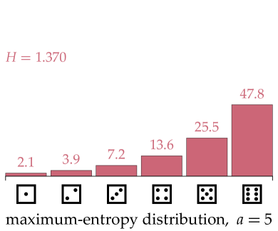
retrodictivepredictive

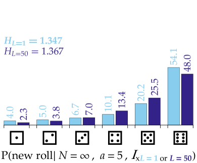
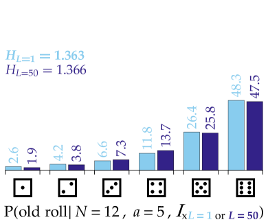
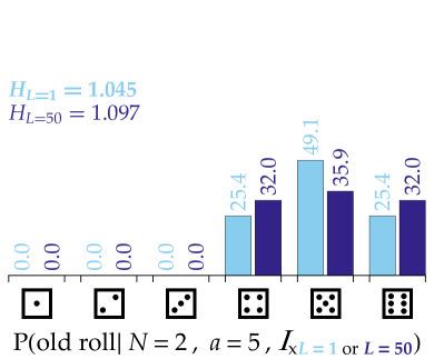
?figurename? 1: Maximum-entropy and exchangeability model, empirical average $a=5$

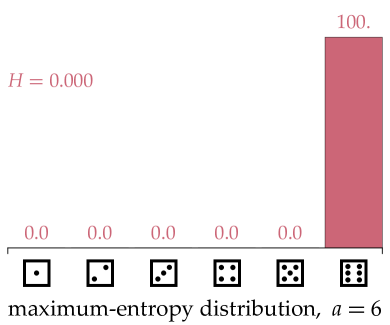
retrodictivepredictive

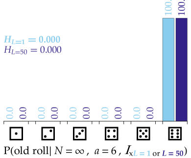
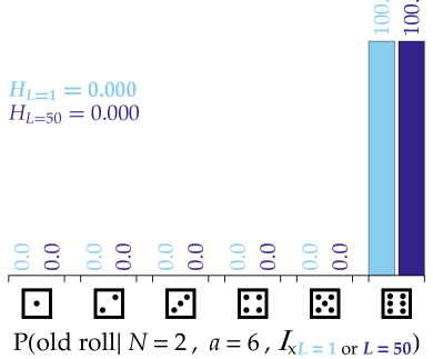
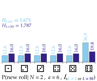
?figurename? 2: Maximum-entropy and exchangeability model, empirical average $a=6$

Their distributions are compared in the classic example of dice rolling in figs 1 and 2 for empirical averages of $5$ and $6$ [portamana2009, see]. The maximum-entropy distribution (red) is at the top; the distribution of the exchangeability model with $L=1$ (blue) and $L=50$ (bluish purple) is shown underneath for the cases $N=2$, $N=12$, $N=\infty$, and for the retrodiction of an “old roll” ${}^{(n)}_{\bm{k}}$, $n\in\{1,\dotsc,N\}$, and the prediction of a “new roll” ${}^{(N+1)}_{\bm{k}}$. The charts also report the Shannon entropies $H$ of the distributions.

The exchangeability model gives very reasonable and even “logical” probabilities for small $N$. For example, if you obtain an average of $5$ in two rolls, it’s impossible that either of them was ⚀ – unless, of course, you own a six-sided die with nine pips on one face. The exchangeability model logically gives zero probability in this case (fig. 1 bottom left). Maximum-entropy gives an erroneous non-zero probability. And having obtained an average of $5$ or $6$ in two rolls, would you really give a much higher probability to ⚄ or ⚅ for a third roll? I’d still give $1/6$. The exchangeability model reasonably gives an almost uniform distribution, especially for large $L$ (both figures bottom right). The maximum-entropy distribution is unreasonably biased towards high values. If we observe a high average in twelve rolls we start to suspect that the die/dice or the roll technique are biased. The exchangeability model expresses this bias, but more conservatively than maximum-entropy.

In fact the predictive exchangeability-model distribution can have higher entropy than the maximum-entropy one! This happens because, when $N$ is small compared to $L$, the maximum-entropy prescription “what you’ve seen in $N$ measurements ${}={}$ what you should expect in an $(N+1)$th measurement” is silly [mackay1995_r2003, Exercise 22.13]. The exchangeability model intelligently doesn’t respect this prescription strictly, if $N$ isn’t large. See Porta Mana *portamana2009 for comparisons under other values of the empirical average and of the number of measurements.

When is $N$ large enough for the prescription to become reasonable? In other words, when is maximum-entropy a good approximation of the exchangeability model with multinomial prior? The answer depends on the interplay among the number of measurements $N$, the number of possible outcomes $K$, the parameter $L$, the reference distribution $\bm{r}$, and the value $a$ (or range $A$) of the observed average. The first three ingredients determine the maximum heights of the densities involved in the integral and sum of eq. (10); the last three ingredients determine the size of the effective integration and sum region relative to the integration simplex, and the distance between the peaks of the data weights and the prior weights of fig.-eq. (26). All five ingredients determine how good are the delta approximations in the integral and sum of eq. (10). We saw in § 2, p. 12, after eq. (12), that $N$ needs to be much larger than $K$ for the integral and delta approximations of the frequency sum to be meaningful. Maximum-entropy approximations are not meaningful if the number of possible outcomes is much larger than the number of observations.

It would be very useful to have explicit estimates of the maximum-entropy-approximation error as a function of the four quantities above. I hope to analyse them in a future note, and promise it would be a shorter note.

5.4 Is this a “derivation” of maximum-entropy?

The heuristic explanation of § 4 shows that the maximum-entropy distributions appear asymptotically owing to our specific choices of a multinomial prior in the exchangeability model, and of an exponential family with observable $\bm{O}$ in the sufficiency model. They are therefore not derived only from first principles or from some sort of universal limit. This is why I don’t call the asymptotic analysis discussed in this note a “derivation” of the maximum-entropy “principle”. In my opinion this analysis shows that it is not a principle at all.

The information-theoretic arguments – or should we say incentives – behind the standard maximum-entropy recipe can be lifted to a meta level and used for priors asymptotically equivalent to the multinomial prior (7), as done by Rodríguez *rodriguez1989,rodriguez2002 for the entropic prior [skilling1989b, skilling1990, see also]. Such arguments don’t determine the parameters $L$ and $\bm{r}$, though. They seem to be prone to an infinite regress; Jaynes was aware of this [jaynes1994_r2003, § 11.1, p. 344].

It would be useful if the multinomial or entropic priors could be uniquely determined by intuitive inferential assumptions, as for example is the case with the Johnson-Dirichlet prior, proportional to $\bm{q}^{L}\,\mathrm{d}\bm{q}$: this prior must be used if we believe (denote this by ${}_{\text{J}}$) that the frequencies of other outcomes are irrelevant for predicting a particular one:

$$\mathrm{p}\bigl{[}{}^{(N+1)}_{k}\mathpunct{\big{|}\ }\bm{f},N,{}_{\text{J}}\bigr{]}=\mathrm{p}\bigl{[}{}^{(N+1)}_{k}\mathpunct{\big{|}\ }f_{k},N,{}_{\text{J}}\bigr{]},\qquad k\in\{1,\dotsc,K\},$$ (28)

a condition called “sufficientness” [johnson1924, johnson1932c][ch. 4]good1965zabell1982,jaynes1986d_r1996. Asymptotically it leads to a maximum-entropy distribution with Burg’s *burg1975 entropy $\mathop{\textstyle\sumop\slimits@}\nolimits\ln\bm{x}$ [jaynes1986d_r1996, portamana2009, see].

But, after all, the logical calculus doesn’t tell us which truths to choose at the beginning of a logical deduction. Why should the probability calculus tell us which probabilities to choose at the beginning of a probabilistic induction?

5.5 Conclusion

Interpreting the maximum-entropy method as an approximation of the exchangeable model (6) with multinomial prior (7) has many advantages:

• it clears up the meaning of the “expectation${}={}$average” prescription of the maximum-entropy method;

• it identifies the range of validity of such prescription;

• it quantifies the error of the maximum-entropy approximation;

• it gives a more sensible solution when this approximation doesn’t hold;

• it clearly differentiates between prediction and retrodiction;

• it can be backed up by information-theoretic incentives [rodriguez1989, rodriguez2002] if you’re into those.

Disadvantages:

• It can’t be used to answer the question “Where did the cat go?”. But this question lies forever beyond the reach of the probability calculus.

That’s all [hanshaw1928].

prenote(“van $X$” is listed under V; similarly for other prefixes, regardless of national conventions.)

postnote