Pain-Free Random Differential Privacy with Sensitivity Sampling

Abstract

Popular approaches to differential privacy, such as the Laplace and exponential mechanisms, calibrate randomised smoothing through global sensitivity of the target non-private function. Bounding such sensitivity is often a prohibitively complex analytic calculation. As an alternative, we propose a straightforward sampler for estimating sensitivity of non-private mechanisms. Since our sensitivity estimates hold with high probability, any mechanism that would be $(\epsilon,\delta)$-differentially private under bounded global sensitivity automatically achieves $(\epsilon,\delta,\gamma)$-random differential privacy (Hall et al., 2012), without any target-specific calculations required. We demonstrate on worked example learners how our usable approach adopts a naturally-relaxed privacy guarantee, while achieving more accurate releases even for non-private functions that are black-box computer programs.

1 Introduction

Differential privacy (Dwork et al., 2006) has emerged as the dominant framework for protected privacy of sensitive training data when releasing learned models to untrusted third parties. This paradigm owes its popularity in part to the strong privacy model provided, and in part to the availability of general building block mechanisms such as the Laplace (Dwork et al., 2006) & exponential (McSherry & Talwar, 2007), and to composition lemmas for building up more complex mechanisms. These generic mechanisms come endowed with privacy and utility bounds that hold for any appropriate application. Such tools almost alleviate the burden of performing theoretical analysis in developing privacy-preserving learners. However a persistent requirement is the need to bound global sensitivity—a Lipschitz constant of the target, non-private function. For simple scalar statistics of the private database, sensitivity can be easily bounded (Dwork et al., 2006). However in many applications—from collaborative filtering (McSherry & Mironov, 2009) to Bayesian inference (Dimitrakakis et al., 2014, 2017; Wang et al., 2015)—the principal challenge in privatisation is completing this calculation.

In this work we develop a simple approach to approximating global sensitivity with high probability, assuming only oracle access to target function evaluations. Combined with generic mechanisms like Laplace, exponential, Gaussian or Bernstein, our sampler enables systematising of privatisation: arbitrary computer programs can be made differentially private with no additional mathematical analysis nor dynamic/static analysis, whatsoever. Our approach does not make any assumptions about the function under evaluation or underlying sampling distribution.

Contributions. This paper contributes: i) SensitivitySamplerfor easily-implemented empirical estimation of global sensitivity of (potentially black-box) non-private mechanisms; ii) Empirical process theory for guaranteeing random differential privacy for any mechanism that preserves (stronger) differential privacy under bounded global sensitivity; iii) Experiments demonstrating our sampler on learners for which analytical sensitivity bounds are highly involved; and iv) Examples where sensitivity estimates beat (pessimistic) bounds, delivering pain-free random differential privacy at higher levels of accuracy, when used in concert with generic privacy-preserving mechanisms.

Related Work. This paper builds on the large body of work in differential privacy (Dwork et al., 2006; Dwork & Roth, 2014), which has gained broad interest in part due the framework’s strong guarantees of data privacy when releasing aggregate statistics or models, and due to availability of many generic privatising mechanisms e.g.,: Laplace (Dwork et al., 2006), exponential (McSherry & Talwar, 2007), Gaussian (Dwork & Roth, 2014), Bernstein (Aldà & Rubinstein, 2017) and many more. While these mechanisms present a path to privatisation without need for reproving differential privacy or utility, they do have in common a need to analytically bound sensitivity—a Lipschitz-type condition on the target non-private function. Often derivations are intricate e.g., for collaborative filtering (McSherry & Mironov, 2009), SVMs (Rubinstein et al., 2012; Chaudhuri et al., 2011), model selection (Thakurta & Smith, 2013), feature selection (Kifer et al., 2012), Bayesian inference (Dimitrakakis et al., 2014, 2017; Wang et al., 2015), SGD in deep learning (Abadi et al., 2016), etc. Undoubtedly the non-trivial nature of bounding sensitivity prohibits adoption by some domain experts. We address this challenge through the SensitivitySampler that estimates sensitivity empirically—even for privatising black-box computer programs—providing high probability privacy guarantees generically.

Several systems have been developed to ease deployment of differentially privacy, with Barthe et al. (2016) overviewing contributions from Programming Languages. Dynamic approaches track privacy budget expended at runtime, typically through basic operations on data with known privacy loss, e.g., the PINQ (McSherry, 2009; McSherry & Mahajan, 2010) and Airavat (Roy et al., 2010) systems. These create a C# LINQ-like interface and a framework for bringing differential privacy to MapReduce, respectively. While such approaches are flexible, the lack of static checking means privacy violations are not caught until after (lengthy) computations. Static checking approaches provide forewarning of privacy usage. In this mould, Fuzz (Reed & Pierce, 2010; Palamidessi & Stronati, 2012) offers a higher-order functional language whose static type system tracks sensitivity based on linear logic, so that sensitivity (and therefore differential privacy) is guaranteed by typechecking. Limited to a similar level of program expressiveness as PINQ, Fuzz cannot typecheck many desirable target programs and specifically cannot track data-dependent function sensitivity, with the DFuzz system demonstrating preliminary work towards this challenge (Gaboardi et al., 2013). While promoting privacy-by-design, such approaches impose specialised languages or limit target feasibility—challenges addressed by this work. Moreover our SensitivitySampler mechanism complements such systems, e.g., within broader frameworks for protecting against side-channel attacks (Haeberlen et al., 2011; Mohan et al., 2012).

Minami et al. (2016) show that special-case Gibbs sampler is $(\epsilon,\delta)$-DP without bounded sensitivity. Nissim et al. (2007) ask: Why calibrate for worst-case global sensitivity when the actual database does not witness worst-case neighbours? Their smoothed sensitivity approach privatises local sensitivity, which itself is sensitive to perturbation. While this can lead to better sensitivity estimates, our sampled sensitivity still does not require analytical bounds. A related approach is the sample-and-aggregate mechanism (Nissim et al., 2007) which avoids computation of sensitivity of the underlying target function and instead requires sensitivity of an aggregator combining the outputs of the non-private target run repeatedly on subsamples of the data. By contrast, our approach provides direct sensitivity estimates, permitting direct privatisation.

Our application of empirical process theory to estimate hard-to-compute quantities resembles the work of Riondato & Upfal (2015). They use VC-theory and sampling to approximate mining frequent itemsets. Here we approximate analytical computations, and to our knowledge provide a first generic mechanism that preserves random differential privacy (Hall et al., 2012)—a natural weakening of the strong guarantee of differential privacy. Hall et al. (2012) leverage empirical process theory for a specific worked example, while our setting is general sensitivity estimation.

2 Background

We are interested in non-private mechanism $f:\mathcal{D}^{n}\to\mathcal{B}$ that maps databases in product space over domain $\mathcal{D}$ to responses in a normed space $\mathcal{B}$. The terminology of “database” (DB) comes from statistical databases, and should be understood as a dataset.

Example 1.

For instance, in supervised learning of linear classifiers, the domain could be Euclidean vectors comprising features & labels, and responses might be parameterisations of learned classifiers such as a normal vector.

We aim to estimate sensitivity which is commonly used to calibrate noise in differentially-private mechanisms.

Definition 2.

The global sensitivity of non-private $f:\mathcal{D}^{n}\to\mathcal{B}$ is given by $\overline{\Delta}=\sup_{D,D^{\prime}}\left\|{f(D)-f(D^{\prime})}\right\|_{\mathcal{B}}$, where the supremum is taken over all pairs of neighbouring databases $D,D^{\prime}$ in $\mathcal{D}^{n}$ that differ in one point.

Definition 3.

Randomized mechanism $M:\mathcal{D}^{n}\to\mathcal{R}$ responding with values in arbitrary response set $\mathcal{R}$ preserves $\epsilon$-differential privacy for $\epsilon>0$ if for all neighbouring $D,D^{\prime}\in\mathcal{D}^{n}$ and measurable $R\subset\mathcal{R}$ it holds that $\mathrm{Pr}\left(M(D)\in R\right)\leq\exp(\epsilon)\mathrm{Pr}\left(M(D^{\prime})\in R\right)$. If instead for $0<\delta<1$ it holds that $\mathrm{Pr}\left(M(D)\in R\right)\leq\exp(\epsilon)\mathrm{Pr}\left(M(D^{\prime})\in R\right)+\delta$ then the mechanism preserves the weaker notion of $(\epsilon,\delta)$-differential privacy.

In Section 4, we recall a number of key mechanisms that preserve these notions of privacy by virtue of target non-private function sensitivity.

The following definition due to Hall et al. (2012) relaxes the requirement that uniform smoothness of response distribution holds on all pairs of databases, to the requirement that uniform smoothness holds for likely database pairs.

Definition 4.

Randomized mechanism $M:\mathcal{D}^{n}\to\mathcal{R}$ responding with values in an arbitrary response set $\mathcal{R}$ preserves $(\epsilon,\gamma)$-random differential privacy, at privacy level $\epsilon>0$ and confidence $\gamma\in(0,1)$, if $\mathrm{Pr}\left(\forall R\subset\mathcal{R},\mathrm{Pr}\left(M(D)\in R\right)\leq e^{\epsilon}\mathrm{Pr}\left(M(D^{\prime})\in R\right)\right)\geq 1-\gamma$, with the inner probabilities over the mechanism’s randomization, and the outer probability over neighbouring $D,D^{\prime}\in\mathcal{D}^{n}$ drawn from some $P^{n+1}$. The weaker $(\epsilon,\delta)$-DP has analogous definition as $(\epsilon,\delta,\gamma)$-RDP.

Remark 5.

While strong $\epsilon$-DP is ideal, utility may demand compromise. Precedent exists for weaker privacy, with the definition of $(\epsilon,\delta)$-DP wherein on any databases (including likely ones) a private mechanism may leak sensitive information on low probability responses, forgiven by the additive $\delta$ relaxation. $(\epsilon,\gamma)$-RDP offers an alternate relaxation, where on all but a small $\gamma$-proportion of unlikely database pairs, strong $\epsilon$-DP holds—RDP plays a useful role.

Example 6.

Consider a database on unbounded positive reals $D\in\mathbb{R}_{+}^{n}$ representing loan default times of a bank’s customers, and target release statistic $f(D)=n^{-1}\sum_{i=1}^{n}D_{i}$ the sample mean. To $\epsilon$-DP privatise scalar-valued $f(D)$ it is natural to look to the Laplace mechanism. However the mechanism requires a bound on the statistic’s global sensitivity, impossible under unbounded $D$. Note for $\Delta>0$, when neighbouring $D,D^{\prime}$ satisfy $\{|f(D)-f(D^{\prime})|\leq\Delta\}$ then Laplace mechanism $M_{\Delta,\epsilon}(f(D))$ enjoys $\epsilon$-DP on that DB pair. Therefore the probability of the latter event is bounded below by the probability of the former. Modelling the default times by iid exponential variables of rate $\lambda>0$, then $|f(D)-f(D^{\prime})|=|D_{n}-D_{n}^{\prime}|/n$ is distributed as $\mathrm{Exp}(n\lambda)$, and so

$$\mathrm{Pr}\left(\forall t\in\mathbb{R},\mathrm{Pr}\left(M_{\Delta,\epsilon}(D)=t\right)\leq e^{\epsilon}\mathrm{Pr}\left(M_{\Delta,\epsilon}(D^{\prime})=t\right)\right)$$

$$\geq \mathrm{Pr}\left(|f(D)-f(D^{\prime})|\leq\Delta\right)=1-e^{-\lambda n\Delta}\geq 1-\gamma\enspace,$$

provided that $\Delta\geq\log(1/\gamma)/(\lambda n)$. While $\epsilon$-DP fails due to unboundedness, the data is likely bounded and so the mechanism is likely strongly private: $M_{\Delta,\epsilon}$ is $(\epsilon,\gamma)$-RDP.

3 Problem Statement

We consider a statistician looking to apply a differentially-private mechanism to an $f:\mathcal{D}^{n}\to\mathcal{B}$ whose sensitivity cannot easily be bounded analytically (cf. Example 6 or the case of a computer program).

Instead we assume that the statistician has the ability to sample from some arbitrary product space $P^{n+1}$ on $\mathcal{D}^{n+1}$, can evaluate $f$ arbitrarily (and in particular on the result of this sampling), and is interested in applying a privatising mechanism with the guarantee of random differential privacy (Definition 4).

Remark 7.

Natural choices for $P$ present themselves for sampling or defining random differential privacy. $P$ could be taken as the underlying distribution from which a sensitive DB was drawn—in the case of sensitive training data but insensitive data source; an alternate test distribution of interest in the case of domain adaptation; or $P$ could be uniform or an otherwise non-informative likelihood (cf. Example 6). Proved in Appendix A, the following relates RDP of similar distributions.

Proposition 8.

Let $P,Q$ be distributions on $\mathcal{D}$ with bounded KL divergence $KL(P\|Q)\leq\tau$. If mechanism $M$ on databases in $\mathcal{D}^{n}$ is RDP with confidence $\gamma>0$ wrt $P$ then it is also RDP with confidence $\gamma+\sqrt{(n+1)\tau/2}$ wrt $Q$, with the same privacy parameters $\epsilon$ (or $\epsilon,\delta$).

4 Sensitivity-Induced Differential Privacy

When a privatising mechanism $M$ is known to achieve differential privacy for some mapping $f:\mathcal{D}^{n}\to\mathcal{B}$ under bounded global sensitivity, then our approach’s high-probability estimates of sensitivity will imply high-probability preservation of differential privacy. In order to reason about such arguments, we introduce the concept of sensitivity-induced differential privacy.

Definition 9.

For arbitrary mapping $f:\mathcal{D}^{n}\to\mathcal{B}$ and randomised mechanism $M_{\Delta}:\mathcal{B}\to\mathcal{R}$, we say that $M_{\Delta}$ is sensitivity-induced $\epsilon$-differentially private if for a neighbouring pair of databases $D,D^{\prime}\in\mathcal{D}^{n}$, and $\Delta\geq 0$

$$\left\|{f(D)-f(D^{\prime})}\right\|_{\mathcal{B}}\leq\Delta$$

$$\Longrightarrow\hskip 10.00002pt \forall R\subset\mathcal{R},\ \mathrm{Pr}\left(M_{\Delta}(f(D))\in R\right)$$

$$\hphantom{\forall R\subset\mathcal{R},\ \ }\leq\ \exp(\epsilon)\cdot\mathrm{Pr}\left(M_{\Delta}(f(D^{\prime}))\in R\right)$$

with the qualification on $R$ being all measurable subsets of the response set $\mathcal{R}$. In the same vein, the analogous definition for $(\epsilon,\delta)$-differential privacy can also be made.

Many generic mechanisms in use today preserve differential privacy by virtue of satisfying this condition. The following are immediate consequences of existing proofs of differential privacy. First, when a non-private target function $f$ aims to release Euclidean vectors responses.

Corollary 10 (Laplace mechanism).

Consider database $D\in\mathcal{D}^{n}$, normed space $\mathcal{B}=(\mathbb{R}^{d},\|\cdot\|_{1})$ for $d\in\mathbb{N}$, non-private function $f:\mathcal{D}^{n}\to\mathcal{B}$. The Laplace mechanism (Dwork et al., 2006) $M_{\Delta}(f(D))\sim\mathrm{Lap}\left(f(D),\Delta/\epsilon\right)$, is sensitivity-induced $\epsilon$-differentially private.

Example 11.

Example 6 used Corollary 10 for RDP of the Laplace mechanism on unbounded bank loan defaults.

Corollary 12 (Gaussian mechanism).

Consider database $D\in\mathcal{D}^{n}$, normed space $\mathcal{B}=(\mathbb{R}^{d},\|\cdot\|_{2})$ for some $d\in\mathbb{N}$, and non-private function $f:\mathcal{D}^{n}\to\mathcal{B}$. The Gaussian mechanism (Dwork & Roth, 2014) $M_{\Delta}(f(D))\sim\mathcal{N}\left(f(D),\mathrm{diag}\left(\sigma\right)\right)$ with $\sigma^{2}>2\Delta^{2}\log(1.25/\delta)/\epsilon^{2}$, is sensitivity-induced $(\epsilon,\delta)$-differentially private.

Second, $f$ may aim to release elements of an arbitrary set $\mathcal{R}$, where a score function $s(D,\cdot)$ benchmarks quality of potential releases (placing a partial ordering on $\mathcal{R}$).

Corollary 13 (Exponential mechanism).

Consider database $D\in\mathcal{D}^{n}$, response space $\mathcal{R}$, normed space $\mathcal{B}=\left(\mathbb{R}^{\mathcal{R}},\|\cdot\|_{\infty}\right)$, non-private score function $s:\mathcal{D}^{n}\times\mathcal{R}\to\mathbb{R}$, and restriction $f:\mathcal{D}^{n}\to\mathcal{B}$ given by $f(D)=s(D,\cdot)$. The exponential mechanism (McSherry & Talwar, 2007) $M_{\Delta}(f(D))\sim\exp\left(\epsilon\left(f(D)\right)(r)/2\Delta\right)$, which when normalised specifies a PDF over responses $r\in\mathcal{R}$, is sensitivity-induced $\epsilon$-differentially private.

Third, $f$ could be function-valued as for learning settings, where given a training set we wish to release a model (e.g., classifier or predictive posterior) that can be subsequently evaluated on (non-sensitive) test points.

Corollary 14 (Bernstein mechanism).

Consider database $D\in\mathcal{D}^{n}$, query space $\mathcal{Y}=[0,1]^{\ell}$ with constant dimension $\ell\in\mathbb{N}$, lattice cover of $\mathcal{Y}$ of size $k\in\mathbb{N}$ given by $\mathcal{L}=\left(\left\{0,1/k,\ldots,1\right\}\right)^{\ell}$, normed space $\mathcal{B}=\left(\mathbb{R}^{\mathcal{Y}},\|\cdot\|_{\infty}\right)$, non-private function $F:\mathcal{D}^{n}\times\mathcal{Y}\to\mathbb{R}$, and restriction $f:\mathcal{D}^{n}\to\mathcal{B}$ given by $f(D)=F(D,\cdot)$. The Bernstein mechanism (Aldà & Rubinstein, 2017) $M_{\Delta}(f(D))\sim\left\{\mathrm{Lap}\left((f(D))(\mathbf{p}),\Delta(k+1)^{\ell}/\epsilon\right)\mid\mathbf{p}\in\mathcal{L}\right\}$, is sensitivity-induced $\epsilon$-differentially private.

Our framework does not apply directly to the objective perturbation mechanism of Chaudhuri et al. (2011), as that mechanism does not rely directly on a notion of sensitivity of objective function, classifier, or otherwise. However it can apply to the posterior sampler used for differentially-private Bayesian inference (Mir, 2012; Dimitrakakis et al., 2014, 2017; Zhang et al., 2016): there the target function $f:\mathcal{D}^{n}\to\mathcal{B}$ returns the likelihood function $p(D|\cdot)$, itself mapping parameters $\Theta$ to $\mathbb{R}$; using the result of $f(D)$ and public prior $\xi(\theta)$, the mechanism samples from the posterior $\xi(B|D)=\int_{B}p(D|\theta)d\xi(\theta)/\int_{\Theta}p(D|\theta)d\xi(\theta)$; differential privacy follows from a Lipschitz condition on $f$ that would require our sensitivity sampler to sample from all database pairs—a minor modification left for future work.

Algorithm 1 SensitivitySampler

  Input: database size $n$, target mapping $f:\mathcal{D}^{n}\to\mathcal{B}$, sample size $m$, order statistic index $k$, distribution $P$

  for $i=1$ to $m$ do

     Sample $D\sim P^{n+1}$

     Set $G_{i}=\left\|{f\left(D_{1\ldots n}\right)-f\left(D_{1\ldots n-1,n+1}\right)}\right\|_{\mathcal{B}}$

  end for

  Sort $G_{1},\ldots,G_{m}$ as $G_{(1)}\leq\ldots\leq G_{(m)}$

  return $\hat{\Delta}=G_{(k)}$

5 The Sensitivity Sampler

Algorithm 1 presents the SensitivitySampler in detail. Consider privacy-insensitive independent sample $D_{1},\ldots,D_{m}\sim P^{n+1}$ of databases on $n+1$ records, where $P$ is chosen to match the desired distribution in definition of random differential privacy. A number of natural choices are available for $P$ (cf. Remark 7). The main idea of SensitivitySampler is that for each extended-database observation of $D\sim P^{n+1}$, we induce i.i.d. observations $G_{1},\ldots,G_{m}\in\mathbb{R}$ of the random variable

$$G = \left\|{f\left(D_{1\ldots n}\right)-f\left(D_{1\ldots n-1;n+1}\right)}\right\|_{\mathcal{B}}\enspace.$$

From these observations of the sensitivity of target mapping $f:\mathcal{D}^{n}\to\mathcal{B}$, we estimate w.h.p. sensitivity that can achieve random differential privacy, for the full suite of sensitivity-induced private mechanisms discussed above.

Algorithm 2 Sample-Then-Respond

  Input: database $D$; randomised mechanism $M_{\Delta}:\mathcal{B}\to\mathcal{R}$; target mapping $f:\mathcal{D}^{n}\to\mathcal{B}$, sample size $m$, order statistic index $k$, distribution $P$

  Set $\hat{\Delta}$ to SensitivitySampler $(|D|,f,m,k,P)$

  respond $M_{\hat{\Delta}}(D)$

If we knew the full CDF of $G$, we would simply invert this CDF to determine the level of sensitivity for achieving any desired $\gamma$ level of random differential privacy: higher confidence would invoke higher sensitivity and therefore lower utility. However as we cannot in general possess the true CDF, we resort to uniformly approximating it w.h.p. using the empirical CDF induced by the sample $G_{1},\ldots,G_{m}$. The guarantee of uniform approximation derives from empirical process theory. Figure 1 provides further intuition behind SensitivitySampler. Algorithm 2 presents Sample-Then-Respond which composes SensitivitySampler with any sensitivity-induced differentially-private mechanism.

Figure 1: Inside SensitivitySampler: the true sensitivity CDF (blue); empirical sensitivity CDF (piecewise constant red); inversion of the empirical CDF (black dotted); where $\rho,\rho^{\prime}$ are the DKW confidence and errors defined in Theorem 15.

Our main result Theorem 15 presents explicit expressions for parameters $m,k$ that are sufficient to guarantee that Sample-Then-Respond achieves $(\epsilon,\delta,\gamma)$-random differential privacy. Under that result the parameter $\rho$, which controls the uniform approximation of the empirical CDF from $G_{1},\ldots,G_{m}$ sample to the true CDF, is introduced as a free parameter. We demonstrate through a series of optimisations in Corollaries 20–21 how $\rho$ can be tuned to optimise either sampling effort $m$, utility via order statistic index $k$, or privacy confidence $\gamma$. These alternative explicit choices for $\rho$ serve as optimal operating points for the mechanism.

5.1 Practicalities

SensitivitySampler simplifies the application of differential privacy by obviating the challenge of bounding sensitivity. As such, it is important to explore any practical issues arising in its implementation. The algorithm itself involves few main stages: sampling databases, measuring sensitivity, sorting, order statistic lookup (inversion), followed by the sensitivity-induced private mechanism.

Sampling. As discussed in Remark 7, a number of natural choices for sampling distribution $P$ could be made. Where a simulation process exists, capable of generating synthetic data approximating $D$, then this could be run. For example in the Bayesian setting (Dimitrakakis et al., 2014), one could use a public conditional likelihood $p(\cdot|\theta)$, parametric family $\Theta$, prior $\xi(\theta)$ and sample from the marginal $\int_{\Theta}p(x|\theta)d\xi(\theta)$. Alternatively, it may suffice to sample from the uniform distribution on $\mathcal{D}$, or Gaussian restricted to Euclidean $\mathcal{D}$. In any of these cases, sampling is relatively straightforward and the choice should consider meaningful random differential privacy guarantees relative to $P$.

Sensitivity Measurement. A trivial stage, given neighbouring databases, measurement could involve expanding a mathematical expression representing a target function, or a computer program such as running a deep learning or computer vision open-source package. For some targets, it may be that running first on one database, covers much of the computation required for the neighbouring database in which case amortisation may improve runtime. The cost of sensitivity measurement will be primarily determined by sample size $m$. Note that sampling and measurement can be trivially parallelised over map-reduce-like platforms.

Sorting, Inversion. Strictly speaking the entire sensitivity sample need not be sorted, as only one order statistic is required. That said, sorting even millions of scalar measurements can be accomplished in under a second on a stock machine. An alternative strategy to inversion as presented, is to take the maximum sensitivity measured so as to maximise privacy without consideration to utility.

Mechanism. It is noteworthy that in settings where mechanism $M_{\Delta}$ is to be run multiple times, the estimation of $\hat{\Delta}$ need not be redone. As such SensitivitySampler could be performed entirely in an offline amortisation stage.

Table 1: Optimal $\rho$ operating points for budgeted resources—$\gamma$ or $m$—minimising $m$, $\gamma$ or $k$; proved in Appendix B.

Budgeted	Optimise	$\rho$	$\gamma$	$m$	$k$
$\gamma\in(0,1)$	$m$	$\exp\left(W_{-1}\left(-\frac{\gamma}{2\sqrt{e}}\right)+\frac{1}{2}\right)$	$\bullet$	$\left\lceil\frac{\log\left(\frac{1}{\rho}\right)}{2(\gamma-\rho)^{2}}\right\rceil$	$\left\lceil m\left(1-\gamma+\rho+\sqrt{\frac{\log\left(\frac{1}{\rho}\right)}{2m}}\right)\right\rceil$
$m\in\mathbb{N},\gamma$	$k$	$\exp\left(\frac{1}{2}W_{-1}\left(-\frac{1}{4m}\right)\right)$	$\geq\rho+\sqrt{\frac{\log\left(\frac{1}{\rho}\right)}{2m}}$	$\bullet$	$\left\lceil m\left(1-\gamma+\rho+\sqrt{\frac{\log\left(\frac{1}{\rho}\right)}{2m}}\right)\right\rceil$
$m\in\mathbb{N}$	$\gamma$	$\exp\left(\frac{1}{2}W_{-1}\left(-\frac{1}{4m}\right)\right)$	$\rho+\sqrt{\frac{\log\left(\frac{1}{\rho}\right)}{2m}}$	$\bullet$	$m$

6 Analysis

For the i.i.d. sample of sensitivities $G_{1},\ldots,G_{m}$ drawn within Algorithm 1, denote the corresponding fixed unknown CDF, and corresponding random empirical CDF, by

$$\Phi\left(g\right) = \mathrm{Pr}\left(G\leq g\right)\enspace,$$

$$\Phi_{m}\left(g\right) = \frac{1}{m}\sum_{i=1}^{m}\mathbf{1}\left[G_{i}\leq g\right]\enspace.$$

In this section we use $\Phi_{m}\left(\Delta\right)$ to bound the likelihood of a (non-private, possibly deterministic) mapping $f:\mathcal{D}^{n}\to\mathcal{R}$ achieving sensitivity $\Delta$. This permits bounding RDP.

Theorem 15.

Consider any non-private mapping $f:\mathcal{D}^{n}\to\mathcal{B}$, any sensitivity-induced $(\epsilon,\delta)$-differentially private mechanism $M_{\Delta}$ mapping $\mathcal{B}$ to (randomised) responses in $\mathcal{R}$, any database $D$ of $n$ records, privacy parameters $\epsilon>0$, $\delta\in[0,1]$, $\gamma\in(0,1)$, and sampling parameters size $m\in\mathbb{N}$, order statistic index $m\geq k\in\mathbb{N}$, approximation confidence $0<\rho<\min\{\gamma,1/2\}$, distribution $P$ on $\mathcal{D}$. If

$$m \geq \frac{1}{2(\gamma-\rho)^{2}}\log\left(\frac{1}{\rho}\right)\enspace,$$ (1)

$$k \geq m\left(1-\gamma+\rho+\sqrt{\log(1/\rho)/(2m)}\right)\enspace,$$ (2)

then Algorithm 2 run with $D,M_{\Delta},f,m,k,P$, preserves $(\epsilon,\delta,\gamma)$-random differential privacy.

Proof.

Consider any $\rho^{\prime}\in(0,1)$ to be determined later, and consider sampling $G_{1},\ldots,G_{m}$ and sorting to $G_{(1)}\leq\ldots\leq G_{(m)}$. Provided that

$$1-\gamma+\rho+\rho^{\prime}\leq 1 \Leftrightarrow \rho^{\prime}\leq\gamma-\rho\enspace,$$ (3)

then the random sensitivity $\hat{\Delta}=G_{(k)}$, where $k=\lceil m(1-\gamma+\rho+\rho^{\prime})\rceil$, is the smallest $\Delta\geq 0$ such that $\Phi_{m}(\Delta)\geq 1-\gamma+\rho+\rho^{\prime}$. That is,

$$\Phi_{m}(\hat{\Delta}) \geq 1-\gamma+\rho+\rho^{\prime}\enspace.$$ (4)

Note that if $1-\gamma+\rho+\rho^{\prime}<0$ then $\hat{\Delta}$ can be taken as any $\Delta$, namely zero. Define the events

$$A_{\Delta} = \left\{\forall R\subset\mathcal{R},\ \mathrm{Pr}\left(M_{\Delta}(f(D))\in R\right)\leq\exp(\epsilon)\cdot\right.$$

$$\hskip 70.0001pt\left.\mathrm{Pr}\left(M_{\Delta}(f(D^{\prime}))\in R\right)+\delta\right\}$$

$$B_{\rho^{\prime}} = \left\{\sup_{\Delta}\left(\Phi_{m}(\Delta)-\Phi(\Delta)\right)\leq\rho^{\prime}\right\}\enspace.$$

The first is the event that DP holds for a specific DB pair, when the mechanism is run with (possibly random) sensitivity parameter $\Delta$; the second records the empirical CDF uniformly one-sided approximating the CDF to level $\rho^{\prime}$. By the sensitivity-induced $\epsilon$-differential privacy of $M_{\Delta}$,

$$\forall\Delta>0\ , \mathrm{Pr}_{D,D^{\prime}\sim P^{n+1}}\left(A_{\Delta}\right)\ \geq\ \Phi(\Delta)\enspace.$$ (5)

The random $D,D^{\prime}$ on the left-hand side induce the distribution on $G$ on the right-hand side under which $\Phi(\Delta)=\mathrm{Pr}_{G}\left(G\leq\Delta\right)$. The probability on the left is the level of random differential privacy of $M_{\Delta}$ when run on fixed $\Delta$. By the Dvoretzky-Kiefer-Wolfowitz inequality (Massart, 1990) we have that for all $\rho^{\prime}\geq\sqrt{(\log 2)/(2m)}$,

$$\mathrm{Pr}_{G_{1},\ldots,G_{m}}\left(B_{\rho^{\prime}}\right)\geq 1-e^{-2m\rho^{\prime 2}}\enspace.$$ (6)

Putting inequalities (4), (5), and (6) together, provided that $\rho^{\prime}\geq\sqrt{(\log 2)/(2m)}$, yields that

Figure 2: The minimum sample size $m$ (sampler effort) required to achieve various target RDP confidence levels $\gamma$.

Figure 3: For sample sizes $m\in\{10^{2},10^{3},10^{4}\}$, trade-offs between privacy confidence level $\gamma$ and order-statistic index $k$ (relative to $m$) which controls sensitivity estimates and so utility.

$$\mathrm{Pr}_{D,D^{\prime},G_{1},\ldots,G_{m}}\left(A_{\hat{\Delta}}\right)$$

$$= \mathbb{E}\left[\left.\mathbf{1}\left[A_{\hat{\Delta}}\right]\right|B_{\rho^{\prime}}\right]\mathrm{Pr}\left(B_{\rho^{\prime}}\right)+\mathbb{E}\left[\left.\mathbf{1}\left[A_{\hat{\Delta}}\right]\right|\overline{B_{\rho^{\prime}}}\right]\mathrm{Pr}\left(\overline{B_{\rho^{\prime}}}\right)$$

$$\geq \mathbb{E}\left[\left.\Phi\left(\hat{\Delta}\right)\right|B_{\rho^{\prime}}\right]\mathrm{Pr}\left(B_{\rho^{\prime}}\right)$$

$$\geq \mathbb{E}\left[\left.\Phi_{m}\left(\hat{\Delta}\right)-\rho^{\prime}\right|B_{\rho^{\prime}}\right]\left(1-\exp\left(-2m\rho^{\prime 2}\right)\right)$$

$$\geq \left(1-\gamma+\rho+\rho^{\prime}-\rho^{\prime}\right)\left(1-\exp\left(-2m\rho^{\prime 2}\right)\right)$$

$$\geq (1-\gamma+\rho)(1-\rho)$$

$$\geq 1-\gamma+\rho-\rho$$

$$= 1-\gamma\enspace.$$

The last inequality follows from $\rho<\gamma$; the penultimate inequality follows from setting

$$\rho^{\prime} \geq \sqrt{\frac{1}{2m}\log\left(\frac{1}{\rho}\right)}\enspace,$$ (7)

and so the DKW condition (Massart, 1990), that $\rho^{\prime}\geq\sqrt{(\log 2)/(2m)}$, is met provided that $\rho\leq 1/2$. Now (1) follows from substituting (7) into (3). ∎

Note that for sensitivity-induced $\epsilon$-differentially private mechanisms, the theorem applies with $\delta=0$.

Optimising Free Parameter $\boldsymbol{\rho}$. Table 1 recommends alternative choices of free parameter $\rho$, derived by optimising the sampler’s performance along one axis—privacy confidence $\gamma$, sampler effort $m$, or order statistic index $k$—given a fixed budget of another. The table summarises results with proofs found in Appendix B. The specific expressions derived involve branches of the Lambert-$W$ function, which is the inverse relation of the function $f(z)=z\exp(z)$, and is implemented as a special function in scientific libraries as standard. While Lambert-$W$ is in general a multi-valued relation on the analytic complex domain, all instances in our results are single-real-valued functions on the reals. The next result presents the first operating point’s corresponding rate on effort in terms of privacy, and follows from recent bounds on the secondary branch $W_{-1}$ due to Chatzigeorgiou (2013).

Corollary 16.

Minimising $m$ for given $\gamma$ (cf. Table 1, row 1; Corollary 20, Appendix B), yields rate for $m$ as $o\left(\frac{1}{\gamma^{2}}\log\frac{1}{\gamma}\right)$ with increasing privacy confidence $\frac{1}{\gamma}\to\infty$.

Remark 17.

Theorem 15 and Table 1 elucidate that effort, privacy and utility are in tension. Effort is naturally decreased by reducing the confidence level of RDP ($\rho$ chosen to minimise $m$, or $\gamma$). By minimising order statistic index $k$, we select smaller $G_{k}$ and therefore sensitivity estimate $\hat{\Delta}$. This in turn leads to lower generic mechanism noise and higher utility. All this is achieved by sacrificing effort or privacy confidence. As usual, sacrificing $\epsilon$ or $\delta$ privacy levels also leads to utility improvement. Figures 2 and 3 visualise these operating points.

Less conservative estimates on sensitivity can lead to superior utility while also enjoying easier implementation. This hypothesis is borne out in experiments in Section 7.

Proposition 18.

For any $f:\mathcal{D}^{n}\to\mathcal{B}$ with global sensitivity $\overline{\Delta}=\sup_{D\sim D^{\prime}}\|f(D)-f(D^{\prime})\|_{\mathcal{B}}$, SensitivitySampler’s random sensitivity $\hat{\Delta}\leq\overline{\Delta}$. As a result, Algorithm 2 run with any of the sensitivity-induced private mechanisms of Corollaries 10–14 achieves utility dominating that of the respective mechanisms run with $\overline{\Delta}$.

Figure 4: Analytical vs estimated sensitivity for Example 6.

7 Experiments

We now demonstrate the practical value of SensitivitySampler. First in Section 7.1 we illustrate how SensitivitySampler sensitivity quickly approaches analytical high-probability sensitivity, and how it can be significantly lower than worst-case global sensitivity in Section 7.2. Running privatising mechanisms with lower sensitivity parameters can mitigate utility loss, while maintaining (a weaker form of) differential privacy. We present experimental evidence of this utility savings in Section 7.3. While application domains may find the alternate balance towards utility appealing by itself, it should be stressed that a significant advantage of SensitivitySampler is its ease of implementation.

7.1 Analytical RDP vs. Sampled Sensitivity

Consider running Example 6: private release of sample mean $f(D)=n^{-1}\sum_{i=1}^{n}D_{i}$ of a database $D$ drawn i.i.d. from $\mathrm{Exp}(1)$. Figure 4 presents, for varying probability $\gamma$: the analytical bound on sensitivity versus SensitivitySampler estimates for different sampling budgets averaged over 50 repeats. For fixed sampling budget, $\hat{\Delta}$ is estimated at lower limits on $\gamma$, quickly converging to exact.

7.2 Global Sensitivity vs. Sampled Sensitivity

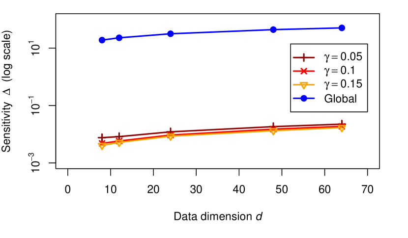
Figure 5: Global vs sampled sensitivity for linear SVM.

Consider now the challenging goal of privately releasing an SVM classifier fit to sensitive training data. In applying the Laplace mechanism to releasing the primal normal vector, Rubinstein et al. (2012) bound the vector’s sensitivity using algorithmic stability of the SVM. In particular, a lengthy derivation establishes that $\|\mathbf{w}_{D}-\mathbf{w}_{D^{\prime}}\|_{1}\leq 4LC\kappa\sqrt{d}/n$ for a statistically consistent formulation of the SVM with convex $L$-Lipschitz loss, $d$-dimensional feature mapping with $\sup_{\mathbf{x}}k(\mathbf{x},\mathbf{x})\leq\kappa^{2}$, and regularisation parameter $C$. While the original work (and others since) did not consider the practical problem of releasing unregularised bias term $b$, we can effectively bound this sensitivity via a short argument in Appendix D.

Figure 6: Linear SVM predictive error under sensitivity estimates vs with global sensitivity bound.

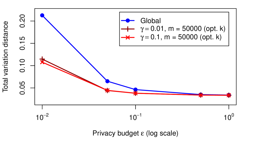
Figure 7: KDE error (relative to non-private) under sensitivity estimates vs global sensitivity bound.

Proposition 19.

For the SVM run with hinge loss, linear kernel, $\mathcal{D}=[0,1]^{d}$, the release $(\mathbf{w},b)$ has $L_{1}$ global sensitivity bounded by $2+2C\sqrt{d}+4Cd/n$.

We train private SVM using the Laplace mechanism (Rubinstein et al., 2012), with global sensitivity bound of Proposition 19 or SensitivitySampler. We synthesise a dataset of $n=1000$ points, selected with equal probability of being drawn from the positive class $N(0.2\cdot\mathbf{1},\mathrm{diag}(0.01))$ or negative class $N(0.8\cdot\mathbf{1},\mathrm{diag}(0.01))$. The feature space’s dimension varies from $d=8$ through $d=64$. The SVMs are run with $C=3$, SensitivitySampler with $m=1500$ & varying $\gamma$. Figure 5 shows very different sensitivities obtained. While estimated $\hat{\Delta}$ hovers around 0.01 largely independent of $\gamma$, global sensitivity $\overline{\Delta}$ exceeds 20—two orders of magnitude greater. These patterns are repeated as dimension increases; sensitivity increasing is to be expected since as dimensions are added, the few points in the training set become more likely to be support vectors and thus affecting sensitivity. Such conservative estimates could clearly lead to inferior utility.

7.3 Effect on Utility

Support Vector Classification. We return to the same SVM setup as in the previous section, with $d=2$, now plotting utility as misclassification error (averaged over 500 repeats) vs. privacy budget $\epsilon$. Here we set $\gamma=0.05$ and include also the non-private SVM’s performance as a bound on utility possible. See Figure 7. At very high privacy levels both private SVMs suffer the same poor error. But quickly with lower privacy, the misclassification error of SensitivitySampler drops until it reaches the non-private rate. Simultaneously the global sensitivity approach has a significantly higher value and suffers a much slower decline. These results suggest that SensitivitySampler can achieve much better utility in addition to sensitivity.

Kernel Density Estimation. We finally consider a one dimensional ($d=1$) KDE setting. In Figure 7 we show the error (averaged over 1000 repeats) of the Bernstein mechanism (with lattice size $k=10$ and Bernstein order $h=3$) on 5000 points drawn from a mixture of two normal distributions $N(0.5,0.02)$ and $N(0.75,0.005)$ with weights $0.4$, $0.6$, respectively. For this experimental result, we set $m=50000$ and two different values for $\gamma$, as displayed in Figure 7. Once again we observe that for high privacy levels the global sensitivity approach incurs a higher error relative to non-private, while SensitivitySampler provides stronger utility. At lower privacy, both approaches converge to the approximation error of the Bernstein polynomial used.

8 Conclusion

In this paper we propose SensitivitySampler, an algorithm for empirical estimation of sensitivity for privatisation of black-box functions. Our work addresses an important usability gap in differential privacy, whereby several generic privatisation mechanisms exist complete with privacy and utility guarantees, but require analytical bounds on global sensitivity (a Lipschitz condition) on the non-private target. While this sensitivity is trivially derived for simple statistics, for state-of-the-art learners sensitivity derivations are arduous e.g., in collaborative filtering (McSherry & Mironov, 2009), SVMs (Rubinstein et al., 2012; Chaudhuri et al., 2011), model selection (Thakurta & Smith, 2013), feature selection (Kifer et al., 2012), Bayesian inference (Dimitrakakis et al., 2014; Wang et al., 2015), and deep learning (Abadi et al., 2016).

While derivations may prevent domain experts from leveraging differential privacy, our SensitivitySampler promises to make privatisation simple when using existing mechanisms including Laplace (Dwork et al., 2006), Gaussian (Dwork & Roth, 2014), exponential (McSherry & Talwar, 2007) and Bernstein (Aldà & Rubinstein, 2017). All such mechanisms guarantee differential privacy on pairs of databases for which a level $\Delta$ of non-private function sensitivity holds, when the mechanism is run with that $\Delta$ parameter. For all such mechanisms we leverage results from empirical process theory to establish guarantees of random differential privacy (Hall et al., 2012) when using sampled sensitivities only.

Experiments demonstrate that real-world learners can easily be run privately without any new derivation whatsoever. And by using a naturally-weaker form of privacy, while replacing worst-case global sensitivity bounds with estimated (actual) sensitivities, we can achieve far superior utility than existing approaches.

Appendix A Proof of Proposition 8

By Pinsker’s inequality the product measures have bounded total variation distance

$$\left\|P^{n+1}-Q^{n+1}\right\|\leq\sqrt{\frac{1}{2}KL\left(P^{n+1}\|Q^{n+1}\right)}\leq\sqrt{\frac{n+1}{2}\tau}.$$

Denote by $A$ the event that $\epsilon$-DP holds (similarly for $(\epsilon,\delta)$-DP) on neighbouring databases on $n$ records:

$$A=\left\{\forall R\subset\mathcal{R},\mathrm{Pr}\left(M(D)\in R\right)\leq e^{\epsilon}\mathrm{Pr}\left(M(D^{\prime})\in R\right)\right\}.$$

Then RDP wrt $Q$ follows as

$$Q^{n+1}(A) \geq P^{n+1}(A)-\sqrt{(n+1)\tau/2}$$

$$\geq 1-\gamma-\sqrt{(n+1)\tau/2}\enspace.$$

Appendix B Optimising Sampler Performance with $\boldsymbol{\rho}$

This section presents precise statements and proofs for the expressions found in Table 1.

B.1 Fixed $\boldsymbol{\gamma}$ Minimum $\boldsymbol{m}$

Corollary 20.

For fixed given privacy confidence budget $\gamma\in(0,1)$, taking

$$\rho = \exp\left(W_{-1}\left(-\frac{\gamma}{2\sqrt{e}}\right)+\frac{1}{2}\right)\enspace,$$

$$m = \left\lceil\left(2(\gamma-\rho)^{2}\right)^{-1}\log(1/\rho)\right\rceil\enspace,$$

$$k = \left\lceil m\left(1-\gamma+\rho+\sqrt{\log(1/\rho)/(2m)}\right)\right\rceil\enspace,$$

minimises sampling effort $m$, when running Algorithm 2 to achieve $(\epsilon,\delta,\gamma)$-RDP.

Proof.

For any fixed $\gamma\in(0,1)$, our task is to minimise the bound

$$m(\rho) = \frac{1}{2(\gamma-\rho)^{2}}\log\frac{1}{\rho}\enspace,$$

on $\rho\in(0,\min\{\gamma,0.5\})$. The first- and second-order derivatives of this function are

$$\frac{\partial m}{\partial\rho} =-\frac{\log\rho}{(\gamma-\rho)^{3}}-\frac{1}{2\rho(\gamma-\rho)^{2}}$$

$$\frac{\partial^{2}m}{\partial\rho^{2}} =-\frac{3\log\rho}{(\gamma-\rho)^{4}}-\frac{2}{\rho(\gamma-\rho)^{3}}+\frac{1}{2\rho^{2}(\gamma-\rho)^{2}}$$

$$=\frac{1}{2\rho^{2}(\gamma-\rho)^{4}}\left[(\gamma-3\rho)^{2}+\rho^{2}\left(6\log\frac{1}{\rho}-4\right)\right].$$

For the second derivative to be positive, it is sufficient for $6\log\frac{1}{\rho}-4>0$ which in turn is guaranteed when $\rho<\exp(-2/3)\approx 0.51$. Therefore $m(\rho)$ is strictly convex on the feasible region; and the first-order necessary condition for optimality is also sufficient. We seek $\rho^{\star}$ critical point

$$0 = -(\gamma-\rho^{\star})^{-2}\left[\frac{\log\rho^{\star}}{\gamma-\rho^{\star}}+\frac{1}{2\rho^{\star}}\right]$$

$$\Leftrightarrow-\frac{\log\rho^{\star}}{\gamma-\rho^{\star}} = \frac{1}{2\rho^{\star}}$$

$$\Leftrightarrow-\gamma = 2\rho^{\star}\log\rho^{\star}-\rho^{\star}$$

$$\Leftrightarrow-\frac{\gamma}{2\sqrt{e}} = \left(\log\rho^{\star}-\frac{1}{2}\right)\frac{\rho^{\star}}{\sqrt{e}}$$

$$= \left(\log\rho^{\star}-\frac{1}{2}\right)\exp\left(\log\rho^{\star}-\frac{1}{2}\right)$$

Applying the Lambert-$W$ function to each side, yields

$$\log(\rho^{\star})-\frac{1}{2} \in W\left(-\frac{\gamma}{2\sqrt{e}}\right)$$

$$\Leftrightarrow\rho^{\star} \in \exp\left(W\left(-\frac{\gamma}{2\sqrt{e}}\right)+\frac{1}{2}\right)\enspace.$$

Figure 8: The branches of the Lambert-W function: primary $W_{0}$ (blue) and secondary $W_{-1}$ (red).

The Lambert-$W$ function is real-valued on $[-\exp(-1),\infty)$, within which it is two-valued on $(-\exp(-1),0)$ and univalued otherwise. As depicted in Figure 8, it consists of a primary branch $W_{0}$ which maps $[-\exp(-1),\infty)$ to $[-1,\infty)$, and a secondary branch $W_{-1}$ which maps $[-\exp(-1),0)$ to $[-1,-\infty)$. Returning to our condition on $\rho^{\star}$, consider that for $\gamma\in(0,1)$ we have that $-\frac{\gamma}{2\sqrt{e}}$ since $2>\sqrt{e}$. On this domain primary $W_{0}\in(-1,0)$ while secondary $W_{-1}\in(-\infty,-1)$ and so the primary branch would yield $\rho^{\star}\in(-\exp(-0.5),\exp(0.5))$ which is disjoint from feasible region $(0,0.5]$. The secondary branch, however, has image in $(0,0.28457\ldots)$ which is feasible. Therefore, we arrive at the $\rho^{\star}$ as claimed, completing the main part of the proof. ∎

B.2 Fixed $\boldsymbol{m}$ and $\boldsymbol{\gamma}$ Minimum $\boldsymbol{k}$

Corollary 21.

For given fixed sampling resource budget $m\in\mathbb{N}$ and privacy confidence $\gamma\in(0,1)$, taking

$$\rho = \exp\left(\frac{1}{2}W_{-1}\left(-\frac{1}{4m}\right)\right)\enspace,$$

$$k = \left\lceil m\left(1-\gamma+\rho+\sqrt{\log(1/\rho)/(2m)}\right)\right\rceil\enspace,$$

provided that

$$\gamma \geq \rho+\sqrt{\log(1/\rho)/(2m)}\enspace,$$

minimises order-statistic index $k$, when running Algorithm 2 to achieve $(\epsilon,\delta,\gamma)$-RDP.

Proof.

For fixed $m,\gamma$, our task is to minimise the bound

$$k(\rho) = m\left(1-\gamma+\rho+\sqrt{\frac{\log(1/\rho)}{2m}}\right)\enspace,$$

or equivalently

$$\tilde{k}(\rho) = \rho+\sqrt{\frac{\log(1/\rho)}{2m}}\enspace,$$ (8)

on $\rho\in(0,\min\{\gamma,0.5\})$. The first- and second-order derivatives of this function are

$$\frac{\partial\tilde{k}}{\partial\rho} =1-\frac{1}{2\sqrt{2m}\rho\sqrt{\log(1/\rho)}}$$

$$\frac{\partial^{2}\tilde{k}}{\partial\rho^{2}} =\frac{1}{2\sqrt{2m}\rho^{2}\sqrt{\log(1/\rho)}}\left[1-\frac{1}{2\log(1/\rho)}\right]\enspace.$$

Since its leading term is positive on feasible $\rho$, it follows that the second derivative is strictly positive iff $\rho<\exp(-1/2)\approx 0.6$ which is guaranteed on the feasible region. Therefore $k(\rho)$ is strictly convex; and the first-order necessary condition for optimality is also sufficient. Next we seek $\rho^{\star}$ critical point

$$0 = 1-\frac{1}{2\sqrt{2m}\rho^{\star}\sqrt{\log(1/\rho^{\star})}}$$

$$\Leftrightarrow\rho^{\star 2}\log\rho^{\star} = -\frac{1}{8m}$$

$$\Leftrightarrow\rho^{\star^{2}}\log\rho^{\star^{2}} = -\frac{1}{4m}$$

$$\Leftrightarrow\log\rho^{\star^{2}} = W\left(-\frac{1}{4m}\right)$$

$$\Leftrightarrow\rho^{\star} \in \exp\left(\frac{1}{2}W\left(-\frac{1}{4m}\right)\right)\enspace,$$

where the introduction of the Lambert-$W$ function leverages the identity $W(z\log z)=\log z$. Since $-\exp(-1)<-(4m)^{-1}<0$ it follows that $W$ is real- and strictly negative in value. Further, since $\rho\leq 0.5<\exp(-1/2)\approx 0.6$, it follows that our solution lies again in the lower branch as claimed.

To guarantee that the relation (1) between $m,\gamma,\rho$ is still satisfied, we can solve the bound on $m$ in terms of $\gamma$:

$$m \geq \frac{1}{2(\gamma-\rho)^{2}}\log\left(\frac{1}{\rho}\right)$$

$$\Leftrightarrow\gamma \geq \rho+\sqrt{\frac{1}{2m}\log\left(\frac{1}{\rho}\right)}\enspace.$$ (9)

Operating with this $\gamma$ establishes all the conditions of Theorem 15. ∎

B.3 Fixed $\boldsymbol{m}$ Minimum $\boldsymbol{\gamma}$

Corollary 22.

For given fixed sampling resource budget $m\in\mathbb{N}$, taking

$$\rho = \exp\left(\frac{1}{2}W_{-1}\left(-\frac{1}{4m}\right)\right)\enspace,$$

$$\gamma = \rho+\sqrt{\log(1/\rho)/(2m)}\enspace,$$

$$k = m\enspace,$$

minimises privacy confidence parameter $\gamma$, when running Algorithm 2 to achieve $(\epsilon,\delta,\gamma)$-RDP.

Proof.

Consider now choosing $\rho$ to minimise $\gamma$, for given fixed $m$ sample size budget, while then taking order statistic index $k$ according to the selected $m,\rho,\gamma$. This corresponds to optimising the expression (9) with respect to $\rho$. Noting that this expression is identical to the objective (8), again the global optimiser must be $\rho^{\star}=\exp(W_{-1}(-1/(4m))/2)$. With this choice of $\gamma$, the necessary $k$ equates to $m$. ∎

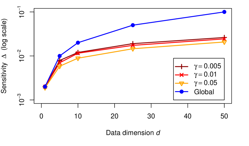
Figure 9: Global vs estimated sensitivity for the sample mean on bounded data.

Appendix C Global vs. Sampled Sensitivity: Sample Mean of Bounded Data

Consider the goal of releasing the sample mean $f(D)=n^{-1}\sum_{i=1}^{n}D_{i}$ of a database $D$ as in Example 6, but over domain $\mathcal{D}=[0,1]^{d}$. Figure 9 presents: the (sharp) bound on global sensitivity for this target for use in e.g., the Laplace mechanism; and the sensitivity $\hat{\Delta}$ estimated by SensitivitySampler. Here $D$ comprises $n=500$ points sampled from the uniform distribution over $\mathcal{D}$, with SensitivitySampler run with optimised $m$ under varying $\gamma$ as displayed. The reduction in sensitivity due to sampling is striking (note the log scale). This experiment demonstrates sensitivity for different privacy guarantees (DP vs. RDP). By contrast for the same level of privacy (RDP) in Section 7.1, SensitivitySampler quickly approaches the analytical approach.

Appendix D Proof of Proposition 19

It follows immediately that $L=1$ and $\kappa=\sqrt{d}$. From the solution $b=y_{i}-\sum_{j=1}^{n}\alpha_{j}y_{j}k(D_{i},D_{j})$ for some $i\in[n]$, combined with the box constraints $0\leq\alpha_{j}\leq C/n$, the sensitivity of the bias can be bounded as $2+2C\sqrt{d}$. Combining with the existing normal vector sensitivity yields the result.

References

- Abadi et al. (2016) Abadi, Martín, Chu, Andy, Goodfellow, Ian, McMahan, H Brendan, Mironov, Ilya, Talwar, Kunal, and Zhang, Li. Deep learning with differential privacy. In Proceedings of the 2016 ACM SIGSAC Conference on Computer and Communications Security, pp. 308–318. ACM, 2016.
- Aldà & Rubinstein (2017) Aldà, Francesco and Rubinstein, Benjamin I. P. The Bernstein mechanism: Function release under differential privacy. In Proceedings of the 31st AAAI Conference on Artificial Intelligence (AAAI’2017), pp. 1705–1711, 2017.
- Barthe et al. (2016) Barthe, Gilles, Gaboardi, Marco, Hsu, Justin, and Pierce, Benjamin. Programming language techniques for differential privacy. ACM SIGLOG News, 3(1):34–53, 2016.
- Chatzigeorgiou (2013) Chatzigeorgiou, Ioannis. Bounds on the Lambert function and their application to the outage analysis of user cooperation. IEEE Communications Letters, 17(8), 2013.
- Chaudhuri et al. (2011) Chaudhuri, Kamalika, Monteleoni, Claire, and Sarwate, Anand D. Differentially private empirical risk minimization. Journal of Machine Learning Research, 12(Mar):1069–1109, 2011.
- Dimitrakakis et al. (2014) Dimitrakakis, Christos, Nelson, Blaine, Mitrokotsa, Aikaterini, and Rubinstein, Benjamin I. P. Robust and private Bayesian inference. In International Conference on Algorithmic Learning Theory, pp. 291–305. Springer, 2014.
- Dimitrakakis et al. (2017) Dimitrakakis, Christos, Nelson, Blaine, Zhang, Zuhe, Mitrokotsa, Aikaterini, and Rubinstein, Benjamin I. P. Differential privacy for Bayesian inference through posterior sampling. Journal of Machine Learning Research, 18(11):1–39, 2017.
- Dwork & Roth (2014) Dwork, Cynthia and Roth, Aaron. The algorithmic foundations of differential privacy. Foundations and Trends in Theoretical Computer Science, 9(3–4):211–407, 2014.
- Dwork et al. (2006) Dwork, Cynthia, McSherry, Frank, Nissim, Kobbi, and Smith, Adam. Calibrating noise to sensitivity in private data analysis. In Theory of Cryptography Conference, pp. 265–284. Springer, 2006.
- Gaboardi et al. (2013) Gaboardi, Marco, Haeberlen, Andreas, Hsu, Justin, Narayan, Arjun, and Pierce, Benjamin C. Linear dependent types for differential privacy. ACM SIGPLAN Notices, 48(1):357–370, 2013.
- Haeberlen et al. (2011) Haeberlen, Andreas, Pierce, Benjamin C, and Narayan, Arjun. Differential privacy under fire. In USENIX Security Symposium, 2011.
- Hall et al. (2012) Hall, Rob, Rinaldo, Alessandro, and Wasserman, Larry. Random differential privacy. Journal of Privacy and Confidentiality, 4(2):43–59, 2012.
- Kifer et al. (2012) Kifer, Daniel, Smith, Adam, and Thakurta, Abhradeep. Private convex empirical risk minimization and high-dimensional regression. Journal of Machine Learning Research, 1(41):3–1, 2012.
- Massart (1990) Massart, Pascal. The tight constant in the Dvoretzky-Kiefer-Wolfowitz inequality. The Annals of Probability, 18(3):1269–1283, 1990.
- McSherry & Mahajan (2010) McSherry, Frank and Mahajan, Ratul. Differentially-private network trace analysis. ACM SIGCOMM Computer Communication Review, 40(4):123–134, 2010.
- McSherry & Mironov (2009) McSherry, Frank and Mironov, Ilya. Differentially private recommender systems: building privacy into the net. In Proceedings of the 15th ACM SIGKDD International Conference on Knowledge Discovery and Data Mining, pp. 627–636. ACM, 2009.
- McSherry & Talwar (2007) McSherry, Frank and Talwar, Kunal. Mechanism design via differential privacy. In 48th Annual IEEE Symposium on Foundations of Computer Science, 2007 (FOCS’07), pp. 94–103. IEEE, 2007.
- McSherry (2009) McSherry, Frank D. Privacy integrated queries: an extensible platform for privacy-preserving data analysis. In Proceedings of the 2009 ACM SIGMOD International Conference on Management of Data, pp. 19–30. ACM, 2009.
- Minami et al. (2016) Minami, Kentaro, Arai, HItomi, Sato, Issei, and Nakagawa, Hiroshi. Differential privacy without sensitivity. In Advances in Neural Information Processing Systems 29, pp. 956–964, 2016.
- Mir (2012) Mir, Darakhshan. Differentially-private learning and information theory. In Proceedings of the 2012 Joint EDBT/ICDT Workshops, pp. 206–210. ACM, 2012.
- Mohan et al. (2012) Mohan, Prashanth, Thakurta, Abhradeep, Shi, Elaine, Song, Dawn, and Culler, David. GUPT: privacy preserving data analysis made easy. In Proceedings of the 2012 ACM SIGMOD International Conference on Management of Data, pp. 349–360. ACM, 2012.
- Nissim et al. (2007) Nissim, Kobbi, Raskhodnikova, Sofya, and Smith, Adam. Smooth sensitivity and sampling in private data analysis. In Proceedings of the Thirty-Ninth Annual ACM Symposium on Theory of Computing, pp. 75–84. ACM, 2007.
- Palamidessi & Stronati (2012) Palamidessi, Catuscia and Stronati, Marco. Differential privacy for relational algebra: improving the sensitivity bounds via constraint systems. In Wiklicky, Herbert and Massink, Mieke (eds.), QAPL - Tenth Workshop on Quantitative Aspects of Programming Languages, volume 85, pp. 92–105, 2012.
- Reed & Pierce (2010) Reed, Jason and Pierce, Benjamin C. Distance makes the types grow stronger: a calculus for differential privacy. ACM Sigplan Notices, 45(9):157–168, 2010.
- Riondato & Upfal (2015) Riondato, Matteo and Upfal, Eli. Mining frequent itemsets through progressive sampling with Rademacher averages. In Proceedings of the 21th ACM SIGKDD International Conference on Knowledge Discovery and Data Mining, pp. 1005–1014. ACM, 2015.
- Roy et al. (2010) Roy, Indrajit, Setty, Srinath TV, Kilzer, Ann, Shmatikov, Vitaly, and Witchel, Emmett. Airavat: Security and privacy for MapReduce. In NSDI, volume 10, pp. 297–312, 2010.
- Rubinstein et al. (2012) Rubinstein, Benjamin I. P., Bartlett, Peter L., Huang, Ling, and Taft, Nina. Learning in a large function space: Privacy-preserving mechanisms for SVM learning. Journal of Privacy and Confidentiality, 4(1):65–100, 2012.
- Thakurta & Smith (2013) Thakurta, Abhradeep Guha and Smith, Adam. Differentially private feature selection via stability arguments, and the robustness of the Lasso. In Conference on Learning Theory, pp. 819–850, 2013.
- Wang et al. (2015) Wang, Yu-Xiang, Fienberg, Stephen E, and Smola, Alexander J. Privacy for free: Posterior sampling and stochastic gradient Monte Carlo. In ICML, pp. 2493–2502, 2015.
- Zhang et al. (2016) Zhang, Zuhe, Rubinstein, Benjamin I. P., and Dimitrakakis, Christos. On the differential privacy of Bayesian inference. In Proceedings of the Thirtieth AAAI Conference on Artificial Intelligence, pp. 2365–2371. AAAI Press, 2016.