Constraints to dark energy using PADE parameterisations

Abstract

We put constraints on dark energy properties using the PADE parameterisation, and compare it to the same constraints using Chevalier-Polarski-Linder (CPL) and $\Lambda$CDM, at both the background and the perturbation levels. The dark energy equation of state parameter of the models is derived following the mathematical treatment of PADE expansion. Unlike CPL parameterisation, the PADE approximation provides different forms of the equation of state parameter which avoid the divergence in the far future. Initially, we perform a likelihood analysis in order to put constraints on the model parameters using solely background expansion data and we find that all parameterisations are consistent with each other. Then, combining the expansion and the growth rate data we test the viability of PADE parameterisations and compare them with CPL and $\Lambda$CDM models respectively. Specifically, we find that the growth rate of the current PADE parameterisations is lower than $\Lambda$CDM model at low redshifts, while the differences among the models are negligible at high redshifts. In this context, we provide for the first time growth index of linear matter perturbations in PADE cosmologies. Considering that dark energy is homogeneous we recover the well known asymptotic value of the growth index, namely $\gamma_{\infty}=\frac{3(w_{\infty}-1)}{6w_{\infty}-5}$, while in the case of clustered dark energy we obtain $\gamma_{\infty}\simeq\frac{3w_{\infty}(3w_{\infty}-5)}{(6w_{\infty}-5)(3w_{\infty}-1)}$. Finally, we generalize the growth index analysis in the case where $\gamma$ is allowed to vary with redshift and we find that the form of $\gamma(z)$ in PADE parameterisation extends that of the CPL and $\Lambda$CDM cosmologies respectively.

=5

1 Introduction

Various independent cosmic observations including those of type Ia supernova (SnIa) (Riess et al., 1998; Perlmutter et al., 1999; Kowalski et al., 2008), cosmic microwave background (CMB) (Komatsu et al., 2009; Jarosik et al., 2011; Komatsu et al., 2011; Planck Collaboration XIV, 2016), large scale structure (LSS), baryonic acoustic oscillation (BAO) (Tegmark et al., 2004; Cole et al., 2005; Eisenstein et al., 2005; Percival et al., 2010; Blake et al., 2011b; Reid et al., 2012), high redshift galaxies (Alcaniz, 2004), high redshift galaxy clusters (Wang & Steinhardt, 1998a; Allen et al., 2004) and weak gravitational lensing (Benjamin et al., 2007; Amendola et al., 2008; Fu et al., 2008) reveal that the present universe experiences an accelerated expansion. Within the framework of General Relativity (GR), the physical origin of the cosmic acceleration can be described by invoking the existence of an exotic fluid with sufficiently negative pressure, the so-called Dark Energy (DE). One possibility is that DE consists of the vacuum energy or cosmological constant $\Lambda$ with constant EoS parameter $w_{\rm\Lambda}=-1$ (Peebles & Ratra, 2003). Alternatively, the fine-tuning and cosmic coincidence problems (Weinberg, 1989; Sahni & Starobinsky, 2000; Carroll, 2001; Padmanabhan, 2003; Copeland et al., 2006) led the scientific community to suggest a time evolving energy density with negative pressure. In those models, the EoS parameter is a function of redshift, $w(z)$ (Caldwell et al., 1998; Erickson et al., 2002; Armendariz-Picon et al., 2001; Caldwell, 2002; Padmanabhan, 2002; Elizalde et al., 2004). A precise measurement of EoS parameter and its variation with cosmic time can provide important clues about the dynamical behavior of DE and its nature (Copeland et al., 2006; Frieman et al., 2008; Weinberg et al., 2013; Amendola et al., 2013).

One possible way to study the EoS parameter of dynamical DE models is via a parameterisation. In literature, one can find many different EoS parameterisations. One of the simplest and earliest parameterisations is the Taylor expansion of $w_{\rm de}(z)$ with respect to redshift $z$ up to first order as: $w_{\rm de}(z)=w_{0}+w_{1}z$ (Maor et al., 2001; Riess et al., 2004). It can also be generalized by considering the second order approximation in Taylor series as: $w_{\rm de}(z)=w_{0}+w_{1}z+w_{2}z^{2}$ (Bassett et al., 2008). However, these two parameterisations diverge at high redshifts. Hence the well-known Chevallier-Polarski-Linder (CPL) parameterisation, $w_{\rm de}(z)=w_{0}+w_{1}(1-a)=w_{0}+w_{1}z/(1+z)$, was proposed (Chevallier & Polarski, 2001; Linder, 2003). The CPL parameterisation can be considered as a Taylor series with respect to $(1-a)$ and was extended to more general case by assuming the second order approximation as: $w_{\rm de}(a)=w_{0}+w_{1}(1-a)+w_{2}(1-a)^{2}$ (Seljak et al., 2005). In addition to CPL formula, some purely phenomenological parameterisations have been proposed more recently. For example $w_{\rm de}(z)=w_{0}+w_{1}z/(1+z)^{\alpha}$, where $\alpha$ is fixed to 2 (Jassal et al., 2005). In this class, the power law $w_{\rm de}(a)=w_{0}+w_{1}(1-a^{\beta})/\beta$ (Barboza et al., 2009) and logarithmic $w_{\rm de}(a)=w_{0}+w_{1}\ln{a}$ (Efstathiou, 1999) parameterisations have been investigated. Another logarithm parameterisation is $w_{\rm de}(z)=w_{0}/[1+b\ln{(1+z)}]^{\alpha}$, where $\alpha$ is taken to be $1$ or $2$ (Wetterich, 2004). Notice that although the CPL is a well-behaved parameterisation at early ($a\ll 1$) and present ($a\sim 1$) epochs, it diverges when the scale factor goes to infinity. This is also a common difficulty for the above phenomenological parameterisations. Recently to solve the divergence, several phenomenological parameterisations have been introduced (see Dent et al., 2009; Frampton & Ludwick, 2011; Feng et al., 2012, for more details). Notice that most of these EoS parameterisations are ad hoc and purely written by hand where there is no mathematical principle or fundamental physics behind them. In this work we focus on the PADE parameterisation ( see section 2), which from the mathematical point of view seems to be more stable: it does not diverge and can be employed at both small and high redshifts. Using the different types of PADE parameterisations to express the EoS parameter of DE $w_{\rm de}$ in terms of redshift $z$, we study the growth of perturbations in the universe.

DE not only accelerate the expansion rate of universe but also change the evolution of growth rate of matter perturbations and consequently the formation epochs of large scale structures of universe (Armendariz-Picon et al., 1999; Garriga & Mukhanov, 1999; Armendariz-Picon et al., 2000; Tegmark et al., 2004; Pace et al., 2010; Akhoury et al., 2011). Moreover, the growth of cosmic structures are also affected by perturbations of DE when we deal with dynamical DE models with time varying EoS parameter $w_{\rm de}\neq-1$ (Erickson et al., 2002; Bean & Doré, 2004; Hu & Scranton, 2004; Basilakos & Voglis, 2007; Ballesteros & Riotto, 2008; Basilakos et al., 2009a; Koivisto & Mota, 2007; Mota et al., 2007; Gannouji et al., 2010; Basilakos et al., 2010; Sapone & Majerotto, 2012; Batista & Pace, 2013; Dossett & Ishak, 2013; Basse et al., 2014; Pace et al., 2014c; Batista, 2014; Basilakos, 2015; Pace et al., 2014b; Nesseris & Sapone, 2014; Mehrabi et al., 2015c, b; Malekjani et al., 2015; Mehrabi et al., 2015a; Malekjani et al., 2017).

In addition to the background geometrical data the data coming from the formation of large scale structures provide a valuable information about the nature of DE. In particular, we can setup a more general formalism in which the background expansion data including SnIa, BAO, CMB shift parameter, Hubble expansion data joined with the growth rate data of large scale structures in order to put constraints on the parameters of cosmology and DE models (see Cooray et al., 2004; Corasaniti et al., 2005; Basilakos et al., 2010; Blake et al., 2011b; Nesseris et al., 2011; Basilakos & Pouri, 2012; Yang et al., 2014; Koivisto & Mota, 2007; Mota et al., 2007; Gannouji et al., 2010; Mota et al., 2008; Llinares et al., 2014; Llinares & Mota, 2013; Contreras et al., 2013; Chuang et al., 2013; Li et al., 2014; Basilakos, 2015; Mehrabi et al., 2015a, b; Basilakos, 2016; Mota et al., 2010; Malekjani et al., 2017; Fay, 2016; Bonilla Rivera & Farieta, 2016).

In this work, following the lines of the above studies and using the latest observational data including the geometrical data set (SnIa, BAO, CMB, big bang nucleosynthesis (BBN), $H(z)$) combined with growth rate data $f(z)\sigma_{8}$, we perform an overall likelihood statistical analysis to place constraints and find best fit values of the cosmological parameters where the EoS parameter of DE is approximated by PADE parameterisations. Previously, the PADE parameterisations have been studied from different observational tests in Cosmology. For example in Gruber & Luongo (2014), the cosmography analysis has been investigated using the PADE approximation. In Wei et al. (2014), the authors proposed several parameterisations for EoS of DE on the basis of PADE approximation. Confronting these EoS parameterisations with the latest geometrical data, they found that the PADE parameterisations can work well (for similar studies, see Aviles et al., 2014; Zaninetti, 2016; Zhou et al., 2016). Here, for the first time, we study the growth of perturbations in PADE cosmologies. After introducing the main ingredients of PADE parameterisations in Sect.2, we study the background evolution of the universe in Sect.(3). We implement the likelihood analysis using the geometrical data to put constraints on the cosmological and model parameters in PADE parameterisations. In Sect.(4), the growth of perturbations in PADE cosmologies is investigated. Then we perform an overall likelihood analysis including the geometrical + growth rate data to place constraints and obtain the best fit values of the corresponding cosmological parameters. Finally we provide the main concussions in Sect.(5).

2 PADE parameterisations

For an arbitrary function $f(x)$, the PADE approximate of order $(m,n)$ is given by the following rational function (Pade, 1892; Baker & Graves-Morris, 1996; Adachi & Kasai, 2012)

$$f(x)=\frac{a_{0}+a_{1}x+a_{2}x^{2}+...+a_{n}x^{n}}{b_{0}+b_{1}x+b_{2}x^{2}+...+b_{n}x^{m}}\;,$$ (1)

where exponents $(m,n)$ are positive and the coefficients $(a_{\rm i},b{\rm{}_{i}})$ are constants. Obviously, for $b_{\rm i}=0$ (with $i\geq 1$) the current approximation reduces to standard Taylor expansion. In this study we focus on three PADE parameterisations introduced as follows (see also Wei et al., 2014).

2.1 PADE (I)

Based on Eq. (1), we first expand the EoS parameter $w_{\rm de}$ with respect to $(1-a)$ up to order $(1,1)$ as follows (see also Wei et al., 2014):

$$w_{\rm de}(a)=\frac{w_{0}+w_{1}(1-a)}{1+w_{2}(1-a)}\;.$$ (2)

From now on we will call the above formula as PADE (I) parameterisation. In terms of redshift $z$, Eq. (2) is written as

$$w_{\rm de}(z)=\frac{w_{0}+(w_{0}+w_{1})z}{1+(1+w_{2})z}\;.$$ (3)

As expected for $w_{2}=0$ Eq. (2) boils down to CPL parameterisation. Unlike CPL parameterisation, here the EoS parameter with $w_{2}\neq 0$ avoids the divergence at $a\to\infty$ (or equivalently at $z=-1$). Using Eq. (2) we find the following special cases regarding the EoS parameter (see also Wei et al., 2014)

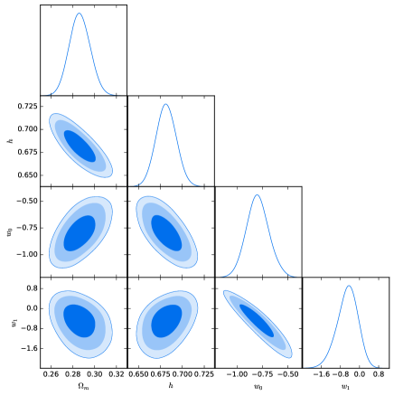
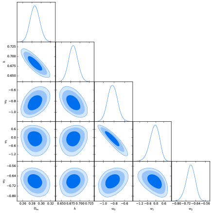
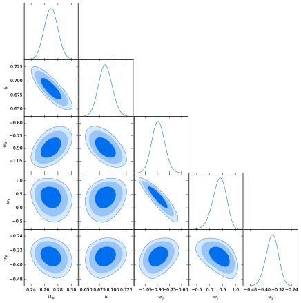
Figure 1: The $1\sigma$, $2\sigma$ and $3\sigma$ likelihood contours for various cosmological parameters using the latest expansion data. The upper left (upper right) panel shows the results for CPL (PADE I) parameterisation. The lower left (lower right) panel shows the results for simplified PADE I (PADE II) parameterisation.

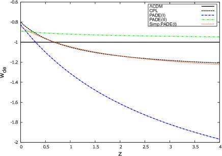
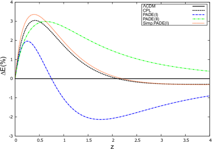
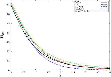
Figure 2: The redshift evolution of various cosmological quantities, namely dark energy EoS parameter $w_{\rm de}(z)$ ( top panel), relative deviation $\Delta E(\%)=[(E-E_{\rm\Lambda})/E_{\rm\Lambda}]\times 100$ (middle panel) and $\Omega_{\rm de}(z)$ ( bottom panel). The different DE parameterisations are characterized by the colors and line-types presented in the inner panels of the figure.

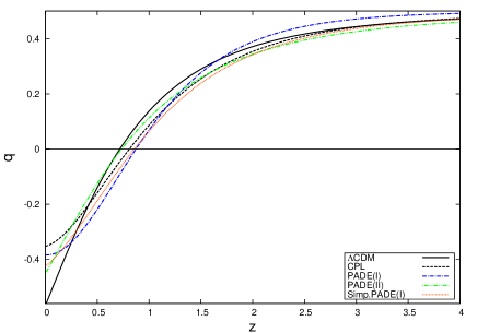
Figure 3: The evolution of the deceleration parameter $q$ for different PADE parameterisations considered in this work. The CPL and $\Lambda$CDM models are shown for comparison.

$$w_{\rm de}=\left\{\begin{array}[]{ll}\frac{w_{0}+w_{1}}{1+w_{2}}\,,\nobreak\leavevmode\nobreak\leavevmode&{\rm for}\leavevmode\nobreak\ \leavevmode\nobreak\ a\to 0\leavevmode\nobreak\ (z\to\infty,\leavevmode\nobreak\ {\rm early\leavevmode\nobreak\ time})\,,\\[11.38109pt] w_{0}\,,&{\rm for}\leavevmode\nobreak\ \leavevmode\nobreak\ a=1\leavevmode\nobreak\ (z=0,\leavevmode\nobreak\ {\rm present})\,,\\[11.38109pt] \frac{w_{1}}{w_{2}}\,,&{\rm for}\leavevmode\nobreak\ \leavevmode\nobreak\ a\to\infty\leavevmode\nobreak\ (z\to-1,\leavevmode\nobreak\ {\rm far\leavevmode\nobreak\ future})\,,\end{array}\right.$$ (7)

where we need to set $w_{2}\not=0$ and $-1$. Therefore, we argue that PADE (I) formula is a well-behaved function in the range of $0\leq a\leq\infty$ (or equivalently at $-1\leq z\leq\infty$ ).

2.2 simplified PADE (I)

Clearly, PADE (I) approximation has three free parameters $w_{0}$, $w_{1}$ and $w_{2}$. Setting $w_{1}=0$ we provide a simplified version of PADE (I) parameterisation, namely

$$w_{\rm de}(a)=\frac{w_{0}}{1+w_{2}(1-a)}\;.$$ (8)

Notice, that in order to avoid singularities in the cosmic expansion $w_{2}$ needs to lie in the interval $-1<w_{2}<0$.

2.3 PADE (II)

Unlike the previous cases, here the current parameterisation is written as a function of $N=\ln{a}$. In this context, the EoS parameter up to order ($1,1$) takes the form

$$w_{\rm de}(a)=\frac{w_{0}+w_{1}\ln{a}}{1+w_{2}\ln{a}}\;,$$ (9)

where $w_{0}$, $w_{1}$ and $w_{2}$ are constants (see also Wei et al., 2014). In PADE (II) parameterisation, we can easily show that

$$w_{\rm de}=\left\{\begin{array}[]{ll}\frac{w_{1}}{w_{2}}\,,\nobreak\leavevmode\nobreak\leavevmode&{\rm for}\leavevmode\nobreak\ \leavevmode\nobreak\ a\to 0\leavevmode\nobreak\ (z\to\infty,\leavevmode\nobreak\ {\rm early\leavevmode\nobreak\ time})\,,\\[11.38109pt] w_{0}\,,&{\rm for}\leavevmode\nobreak\ \leavevmode\nobreak\ a=1\leavevmode\nobreak\ (z=0,\leavevmode\nobreak\ {\rm present})\,,\\[11.38109pt] \frac{w_{1}}{w_{2}}\,,&{\rm for}\leavevmode\nobreak\ \leavevmode\nobreak\ a\to\infty\leavevmode\nobreak\ (z\to-1,\leavevmode\nobreak\ {\rm far\leavevmode\nobreak\ future})\,,\end{array}\right.$$ (13)

Notice, that in order to avoid singularities at the above epochs we need to impose $w_{2}\neq 0$.

Table 1: The statistical results for the various DE parameterisations used in the analysis. These results are based on the expansion data. The concordance $\Lambda$CDM model is shown for comparison.

Model	PADE I	simp. PADE I	PADE II	CPL	$\Lambda$CDM
$k$	6	5	6	5	3
$\chi^{2}_{\rm min}$	567.6	567.7	567.9	567.6	574.4
AIC	579.6	577.7	579.9	577.6	580.4
BIC	606.1	599.8	606.4	599.7	593.6

3 background history in PADE parameterisations

In this section based on the aforementioned parameterisations we study the background evolution in PADE cosmologies. Generally speaking, for isotropic and homogeneous spatially flat FRW cosmologies, driven by radiation, non-relativistic matter and an exotic fluid with an equation of state $p_{\rm de}=w_{\rm de}\rho_{\rm de}$, the first Friedmann equation reads

$$H^{2}=\frac{8\pi G}{3}(\rho_{\rm r}+\rho_{\rm m}+\rho_{\rm de})\;,$$ (14)

where $H\equiv{\dot{a}}/a$ is the Hubble parameter, $\rho_{\rm r}$, $\rho_{\rm m}$ and $\rho_{\rm de}$ are the energy densities of radiation, dark matter and DE, respectively. In the absence of interactions among the three fluids the corresponding energy densities satisfy the following differential equations

$$\dot{\rho_{\rm r}}+4H\rho_{\rm r}=0\;,$$ (15)

$$\dot{\rho_{\rm m}}+3H\rho_{\rm m}=0\;,$$ (16)

$$\dot{\rho_{\rm de}}+3H(1+w_{\rm de})\rho_{\rm de}=0\;,$$ (17)

where the over-dot denotes a derivative with respect to cosmic time $t$. Based on Eqs. (15) and (16), it is easy to derive the evolution of radiation and pressure-less matter, namely $\rho_{\rm r}=\rho_{\rm r0}a^{-4}$ and $\rho_{\rm m}=\rho_{\rm m0}a^{-3}$. Inserting Eqs . (2), (8) and (9) into equation (17), we can obtain the DE density of the current PADE parameterisations (see also Wei et al., 2014)

$$\rho_{\rm de}^{(\rm PADEI)}=\rho^{(0)}_{\rm de}a^{-3(\frac{1+w_{0}+w_{1}+w_{2}}{1+w_{2}})}[1+w_{2}(1-a)]^{-3(\frac{w_{1}-w_{0}w_{2}}{w_{2}(1+w_{2})})}\;,$$ (18)

$$\rho_{\rm de}^{(\rm simp.PADEI)}=\rho^{(0)}_{\rm de}a^{-3(\frac{1+w_{0}+w_{2}}{1+w_{2}})}[1+w_{2}(1-a)]^{-3(\frac{-w_{0}w_{2}}{w_{2}(1+w_{2})})}\;,$$ (19)

$$\rho_{\rm de}^{(\rm padeII)}=\rho^{0}_{\rm de}a^{-3(\frac{w_{1}+w_{2}}{w_{2}})}(1+w_{2}\ln a)^{3(\frac{w_{1}-w_{0}w_{2}}{{w_{2}}^{2}})}\;.$$ (20)

Also, combining Eqs.(18, 19, 20) and Eq.(14) we derive the dimensionless Hubble parameter $E=H/H_{0}$ (see also Wei et al., 2014). Specifically, we find

$$E^{2}_{\rm PADEI}=\Omega_{\rm r0}a^{-4}+\Omega_{\rm m0}a^{-3}+(1-[\Omega_{\rm r0}+\Omega_{\rm m0}])\times$$

$$a^{-3(\frac{1+w_{0}+w_{1}+w_{2}}{1+w_{2}})}\times(1+w_{2}-aw_{2})^{-3(\frac{w_{1}-w_{0}w_{2}}{w_{2}(1+w_{2})})}\;,$$ (21)

$$E^{2}_{\rm simPADEI}=\Omega_{\rm r0}a^{-4}+\Omega_{\rm m0}a^{-3}+(1-[\Omega_{\rm r0}+\Omega_{\rm m0}])\times$$

$$a^{-3(\frac{1+w_{0}+w_{2}}{1+w_{2}})}\times(1+w_{2}-aw_{2})^{-3(\frac{-w_{0}w_{2}}{w_{2}(1+w_{2})})}\;,$$ (22)

$$E^{2}_{\rm PADEII}=\Omega_{\rm r0}a^{-4}+\Omega_{\rm m0}a^{-3}+(1-[\Omega_{\rm r0}+\Omega_{\rm m0}])\times$$

$$a^{-3(\frac{w_{1}+w_{2}}{w_{2}})}\times(1+w_{2}\ln a)^{3(\frac{w_{1}-w_{0}w_{2}}{{w_{2}}^{2}})}\;,$$ (23)

where $\Omega_{\rm m0}$ (density parameter), $\Omega_{\rm r0}$ (radiation parameter) and $\Omega_{\rm de0}=1-\Omega_{\rm m0}-\Omega_{\rm r0}$ (dark energy parameter). Moreover, following the above lines in the case of CPL parameterisation we have

$$\rho^{\rm CPL}_{\rm de}=\rho^{(0)}_{\rm de}a^{-3(1+w_{0}+w_{1})}\exp\{-3w_{1}(1-a)\}$$ (24)

and

$$E^{2}_{\rm CPL}=\Omega_{\rm r0}a^{-4}+\Omega_{\rm m0}a^{-3}+(1-\Omega_{\rm m0}-\Omega_{\rm r0})\times$$

$$a^{-3(1+w_{0}+w_{1})}\exp[{-3w_{1}(1-a)}]\;,$$ (25)

Bellow, we study the performance of PADE cosmological parameterisation against the latest observational data. Specifically, we implement a statistical analysis using the background expansion data including those of SnIa (Suzuki et al., 2012), BAO (Beutler et al., 2011; Padmanabhan et al., 2012; Anderson et al., 2013; Blake et al., 2011a), CMB (Hinshaw et al., 2013), BBN (Serra et al., 2009; Burles et al., 2001), Hubble data (Moresco et al., 2012; Gaztanaga et al., 2009; Blake et al., 2012; Anderson et al., 2014). For more details concerning the expansion data, the $\chi^{2}(\textbf{p})$ function, the Markov chain Monte Carlo (MCMC) analysis, the Akaike information criterion (AIC) and the Bayesian information criterion (BIC) we refer the reader to Mehrabi et al. (2015b) (see also Basilakos et al., 2009b; Hinshaw et al., 2013; Mehrabi et al., 2015a, 2017; Malekjani et al., 2017). In this framework, the joint likelihood function is the product of the individual likelihoods:

$${\cal L}_{\rm tot}({\bf p})={\cal L}_{\rm sn}\times{\cal L}_{\rm bao}\times{\cal L}_{\rm cmb}\times{\cal L}_{\rm h}\times{\cal L}_{\rm bbn}\;,$$ (26)

which implies that the total chi-square $\chi^{2}_{\rm tot}$ is given by:

$$\chi^{2}_{\rm tot}({\bf p})=\chi^{2}_{\rm sn}+\chi^{2}_{\rm bao}+\chi^{2}_{\rm cmb}+\chi^{2}_{\rm h}+\chi^{2}_{\rm bbn}\;,$$ (27)

where the statistical vector ${\bf p}$ includes the free parameters of the model. In our work the above vector becomes (a) ${\bf p}=\{\Omega_{\rm DM0},\Omega_{\rm b0},h,w_{0},w_{1},w_{2}\}$ for PADE (I) and (II) parameterisations, (b) ${\bf p}=\{\Omega_{\rm DM0},\Omega_{\rm b0},h,w_{0},w_{2}\}$ for simplified PADE (I) and (c) ${\bf p}=\{\Omega_{\rm DM0},\Omega_{\rm b0},h,w_{0},w_{1}\}$ in the case of CPL parameterisation. Notice that we utilize $\Omega_{\rm m0}=\Omega_{\rm DM0}+\Omega_{\rm b0}$ and $h=H_{0}/100$, while the energy density of radiation is fixed to $\Omega_{\rm r0}=2.469\times 10^{-5}h^{-2}(1.6903)$ (Hinshaw et al., 2013).

Additionally, we utilize the well know information criteria, namely AIC (Akaike, 1974) and BIC (Schwarz, 1978) in order to test the statistical performance of the cosmological models themselves. In particular, AIC and BIC are given by

$${\rm AIC}=-2\ln{\cal L}_{\rm max}+2k\;,$$

$${\rm BIC}=-2\ln{\cal L}_{\rm max}+k\ln N\;,$$ (28)

where $k$ is the number of free parameters and $N$ is the total number of observational data points. The results of our statistical analysis are presented in Tables (1) and (2) respectively. Although the current DE parameterisations provide low AIC values with respect to those of $\Lambda$CDM, we find $\Delta{\rm AIC}={\rm AIC}-{\rm AIC}_{\rm\Lambda}<4$ hence, the DE parameterisations explored in this study are consistent with the expansion data. In order to visualize the solution space of the model parameters in Fig.(1) we present the $1\sigma$, $2\sigma$ and $3\sigma$ confidence levels for various parameter pairs. Using the best fit model parameters [see Table 2] in Fig. (2) we plot the redshift evolution of $w_{\rm de}$ (upper panel), $\Delta E(\%)=[(E-E_{\rm\Lambda})/E_{\rm\Lambda}]\times 100$ (middle panel) and $\Omega_{\rm de}$ (lower panel). The different parameterisations are characterized by the colors and line-types presented in the caption of Fig. (2). We find that the EoS parameter of PADE II evolves only in the quintessence regime ($-1<w_{\rm de}<-1/3$). For the other DE parameterisations we observe that $w_{\rm de}$ varies in the phantom region ($w_{\rm de}<-1$) at high redshifts, while it enters in the quintessence regime ($-1<w_{\rm de}<-1/3$) at relatively low redshifts. Notice, that the present value of $w_{\rm de}$ can be found in Table (2). From the middle panel of Fig. (2), we observe that the relative difference $\Delta E$ is close to $2-3.5\%$ at low redshifts ($z\sim 0.5$), while in the case of PADE (II) we always have $E_{\rm PADEII}(z)>E_{\rm\Lambda}(z)$. Lastly, in the bottom panel of Fig.(2) we show the evolution of $\Omega_{\rm de}$, where its current value can be found in Table (2). As expected, $\Omega_{\rm de}$ tends to zero at high redshifts since matter dominates the cosmic fluid. In the case of PADE parameterisations we observe that $\Omega_{\rm de}$ is larger than that of the usual $\Lambda$ cosmology.

Finally, we would like to estimate the transition redshift $z_{\rm tr}$ of the PADE parameterisations by utilizing the deceleration parameter $q(z)=-1-\dot{H}/H^{2}$. Following, standard lines it is easy to show

$$\frac{\dot{H}}{H^{2}}=-\frac{3}{2}\Big{(}1+w_{\rm de}(z)\Omega_{\rm de}(z)\Big{)}$$ (29)

which implies that

$$q(z)=\frac{1}{2}+\frac{3}{2}w_{\rm de}(z)\Omega_{\rm de}(z)$$ (30)

Using the best fit values of Table (2), we plot in Fig. (3) the evolution of $q$ for the current DE parameterisations. In all cases, including that of $\Lambda$CDM, $q$ tends to 1/2 at early enough times. This is expected since the universe is matter dominated ($\Omega_{\rm de}\simeq 0$) at high redshifts. Now solving the $q(z_{\rm tr})=0$ we can derive the transition redshift, namely the epoch at which the expansion of the universe starts to accelerate. In particular, we find $z_{\rm tr}=0.86$ (PADE I), $z_{\rm tr}=0.84$ (simplified PADE ), $z_{\rm tr}=0.72$ (PADE II), $z_{\rm tr}=0.80$ (CPL) and $z_{\rm tr}=0.71$ ($\Lambda$CDM). The latter results are in good agreement with the measured $z_{\rm tr}$ based on the cosmic chronometer $H(z)$ data Farooq et al. (2017) (see also Capozziello et al., 2014, 2015).

Table 2: A summary of the best-fit parameters for the various DE parameterisations using the background data.

Model	PADE I	simplified PADE I	PADE II	CPL	$\Lambda$CDM
$\Omega_{\rm m}^{(0)}$	$0.286\pm 0.010$	$0.270\pm 0.010$	$0.2864\pm 0.0096$	$0.2896\pm 0.0090$	$0.2891\pm 0.0090$
$h$	$0.682\pm 0.012$	$0.682\pm 0.012$	$0.686\pm 0.013$	$0.682\pm 0.012$	$0.6837\pm 0.0084$
$w_{0}$	$-0.825\pm 0.091$	$-0.845\pm 0.039$	$-0.889\pm 0.080$	$-0.80\pm 0.11$	$-$
$w_{1}$	$-0.09^{+0.39}_{-0.32}$	$-$	$0.37^{+0.29}_{-0.23}$	$-0.51^{+0.48}_{-0.38}$	$-$
$w_{2}$	$-0.683^{+0.040}_{-0.034}$	$-0.387\pm 0.034$	$-0.353^{+0.038}_{-0.034}$	$-$	$-$
$w_{\rm de}(z=0)$	$-0.825$	$-0.845$	$-0.889$	$-0.80$	$-1.0$
$\Omega_{\rm de}(z=0)$	$0.714$	$0.730$	$0.7136$	$0.7104$	$0.7109$

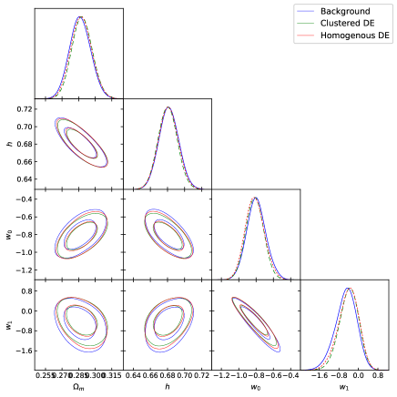
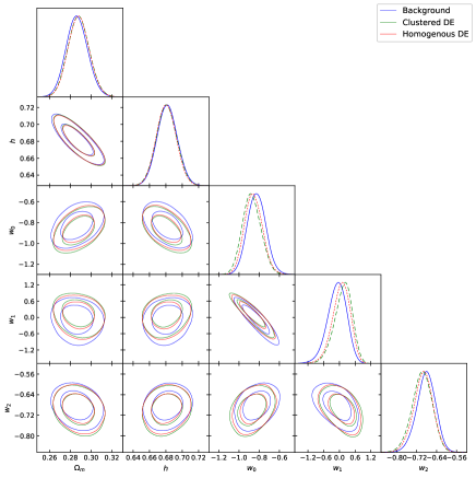
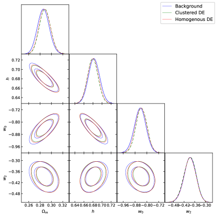
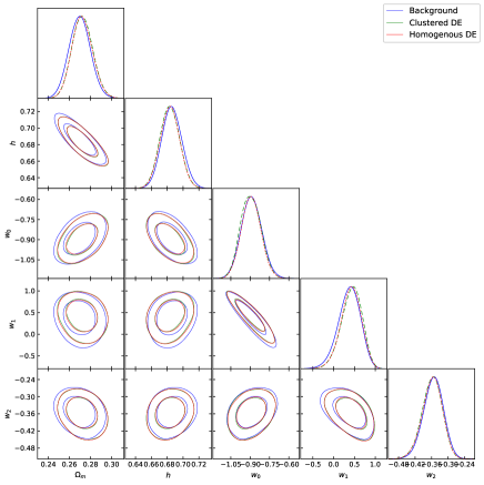
Figure 4: The $1\sigma$ and $2\sigma$ likelihood contours for various planes using the solely expansion data (blue), combined expansion and growth rate data for clustered (green) and homogeneous (red) DE parameterisations. The upper left (upper right) shows the results for CPL (PADE I) parameterisation. The lower left (lower right) shows the results for simplified PADE I (PADE II) parameterisation.

Table 3: The statistical results for homogeneous (clustered) DE parameterisations used in the analysis. These results are based on the expansion+growth rate data. The concordance $\Lambda$CDM model is shown for comparison.

Model	PADE I	simplified PADE I	PADE II	CPL	$\Lambda$CDM
$k$	7	6	7	6	4
$\chi^{2}_{\rm min}$	576.4(576.5)	576.4(576.7)	576.9(577.1)	576.5(576.7)	582.6
AIC	590.4(590.5)	588.4(588.7)	590.9(591.1)	588.5(588.7)	590.6
BIC	621.6(621.7)	615.1(615.4)	622.1(622.3)	615.2(615.4)	608.4

Table 4: A summary of the best-fit parameters for homogeneous (clustered) DE parameterisations using the background+growth rate data.

Model	PADE I	simplified PADE I	PADE II	CPL	$\Lambda$CDM
$\Omega_{\rm m}^{(0)}$	$0.288\pm 0.010\leavevmode\nobreak\ (0.288\pm 0.010)$	$0.288\pm 0.010\leavevmode\nobreak\ (0.2888\pm 0.0099)$	$0.2721\pm 0.0097\leavevmode\nobreak\ (0.2723\pm 0.0098)$	$0.2875\pm 0.0095\leavevmode\nobreak\ (0.2882\pm 0.0093)$	$0.2902\pm 0.0090$
$h$	$0.681\pm 0.012\leavevmode\nobreak\ (0.681\pm 0.012)$	$0.680\pm 0.012\leavevmode\nobreak\ (0.679\pm 0.012)$	$0.684\pm 0.012\leavevmode\nobreak\ (0.683\pm 0.012)$	$0.681\pm 0.011\leavevmode\nobreak\ (0.680\pm 0.011)$	$0.6833\pm 0.0084$
$w_{0}$	$-0.856\pm 0.088\leavevmode\nobreak\ (-0.874^{+0.086}_{-0.097})$	$-0.839\pm 0.038\leavevmode\nobreak\ (-0.836\pm 0.037)$	$-0.893\pm 0.075\leavevmode\nobreak\ (-0.896\pm 0.078)$	$-0.81^{+0.10}_{-0.12}\leavevmode\nobreak\ (-0.81\pm 0.10)$	$-$
$w_{1}$	$0.07^{+0.37}_{-0.29}\leavevmode\nobreak\ (0.14^{+0.38}_{-0.29})$	$-$	$0.41^{+0.26}_{-0.22}\leavevmode\nobreak\ (0.43^{+0.27}_{-0.22})$	$-0.41^{+0.46}_{-0.37}\leavevmode\nobreak\ (-0.39^{+0.42}_{-0.36})$	$-$
$w_{2}$	$-0.694^{+0.040}_{-0.036}\leavevmode\nobreak\ (-0.699^{+0.042}_{-0.038})$	$-0.388\pm 0.034\leavevmode\nobreak\ (-0.388\pm 0.035)$	$-0.357^{+0.039}_{-0.033}\leavevmode\nobreak\ (-0.358^{+0.038}_{-0.034})$	$-$	$-$
$\sigma_{8}$	$0.751\pm 0.015\leavevmode\nobreak\ (0.755\pm 0.016)$	$0.751\pm 0.015\leavevmode\nobreak\ (0.758\pm 0.015)$	$0.771\pm 0.015\leavevmode\nobreak\ (0.771\pm 0.016)$	$0.751\pm 0.015\leavevmode\nobreak\ (0.756\pm 0.015)$	$0.744\pm 0.014$
$w_{\rm de}(z=0)$	$-0.856(-0.874)$	$-0.839(-0.836)$	$-0.893(-0.896)$	$-0.81(-0.81)$	$-1.0$
$\Omega_{\rm de}(z=0)$	$0.712(0.712)$	$0.712(0.7112)$	$0.7279(0.7277)$	$0.7125(0.7118)$	$0.7098$

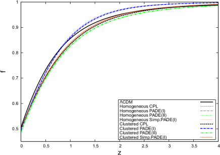
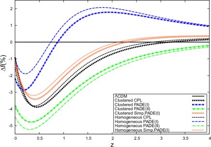
Figure 5: The redshift evolution of the growth rate function $f(z)$ (top-panel) and the corresponding fractional difference $\Delta f(\%)=100\times[f(z)-f_{\rm\Lambda}(z)]/f_{\rm\Lambda}(z)$ (bottom panel). The different DE parameterisations are characterized by the colors and line-types presented in the inner panels of the figure

.

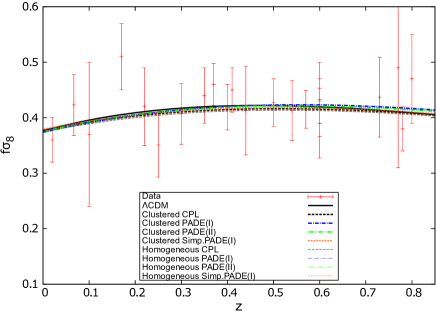
Figure 6: Comparison of the observed and theoretical evolution of the growth rate $f(z)\sigma_{8}(z)$ as a function of redshift $z$. Open squares correspond to the data. Line-types and colors are explained in the inner plot of the figure.

4 Growth rate in DE parameterisations

In this section, we study the linear growth of matter perturbations in PADE cosmologies and we compare them with those of CPL and $\Lambda$CDM respectively. In this kind of studies the natural question to ask is the following: how DE affects the linear growth of matter fluctuations? In order to treat to answer this question we need to introduce the following two distinct situations, which have been considered within different approaches in the literature (Armendariz-Picon et al., 1999; Garriga & Mukhanov, 1999; Armendariz-Picon et al., 2000; Erickson et al., 2002; Bean & Doré, 2004; Hu & Scranton, 2004; Abramo et al., 2007, 2008; Ballesteros & Riotto, 2008; Abramo et al., 2009; Basilakos et al., 2009a; de Putter et al., 2010; Pace et al., 2010; Akhoury et al., 2011; Sapone & Majerotto, 2012; Pace et al., 2012; Batista & Pace, 2013; Dossett & Ishak, 2013; Batista, 2014; Basse et al., 2014; Pace et al., 2014a, c, b; Malekjani et al., 2015; Naderi et al., 2015; Mehrabi et al., 2015c, b, a; Nazari-Pooya et al., 2016; Malekjani et al., 2017): (i) the scenario in which the DE component is homogeneous ($\delta_{\rm de}\equiv 0$) and only the corresponding non-relativistic matter is allowed to cluster ($\delta_{\rm m}\neq 0$) and (ii) the case in which the whole system clusters (both matter and DE). Owing to the fact that we are in the matter phase of the universe we can neglect the radiation term from the Hubble expansion.

4.1 Basic equations

The basic equations that govern the evolution of non-relativistic matter and DE perturbations are given by (Abramo et al., 2009)

$$\dot{\delta_{\rm m}}+\frac{\theta_{\rm m}}{a}=0\;,$$ (31)

$$\dot{\delta_{\rm de}}+(1+w_{\rm de})\frac{\theta_{\rm de}}{a}+3H(c_{\rm eff}^{2}-w_{\rm de})\delta_{\rm de}=0\;,$$ (32)

$$\dot{\theta_{\rm m}}+H\theta_{\rm m}-\frac{k^{2}\phi}{a}=0\;,$$ (33)

$$\dot{\theta_{\rm de}}+H\theta_{\rm de}-\frac{k^{2}c_{\rm eff}^{2}\theta_{\rm de}}{(1+w_{\rm de})a}-\frac{k^{2}\phi}{a}=0\;,$$ (34)

where $k$ is the wave number and $c_{\rm eff}$ is the effective sound speed of perturbations (Abramo et al., 2009; Batista & Pace, 2013; Batista, 2014). Combining the Poisson equation

$$-\frac{k^{2}}{a^{2}}\phi=\frac{3}{2}H^{2}[\Omega_{\rm m}\delta_{\rm m}+(1+3c_{\rm eff}^{2})\Omega_{\rm de}\delta_{\rm de}]\;,$$ (35)

with Eqs. (33 & 34), eliminating $\theta_{\rm m}$ and $\theta_{\rm de}$ and changing the derivative from time to scale factor $a$, we obtain the following stystem of differential equations (see also Mehrabi et al., 2015a; Malekjani et al., 2017)

$$\delta_{\rm m}^{\prime\prime}+\frac{3}{2a}(1-w_{\rm de}\Omega_{\rm de})\delta_{\rm m}^{\prime}=\frac{3}{2a^{2}}[\Omega_{\rm m}\delta_{\rm m}+\Omega_{\rm de}(1+3c_{\rm eff}^{2})\delta_{\rm de}]\;,$$ (36)

$$\delta_{\rm de}^{\prime\prime}+A\delta_{\rm de}^{\prime}+B\delta_{\rm de}=\frac{3}{2a^{2}}(1+w_{\rm de})[\Omega_{\rm m}\delta_{\rm m}+\Omega_{\rm de}(1+3c_{\rm eff}^{2})\delta_{\rm de}]\;.$$ (37)

Bellow we set $c_{\rm eff}\equiv 0$ which means that the whole system (matter and DE) fully clusters. Moreover, we remind reader that for homogeneous DE models we have $\delta_{\rm de}\equiv 0$, hence Eq.(36) reduces to the well known differential equation of Peebles (1993) [see also Pace et al. (2010) and references therein]. Concerning the functional forms of $A$ and $B$ we have

$$A=\frac{1}{a}[-3w_{\rm de}-\frac{aw_{\rm de}^{\prime}}{1+w_{\rm de}}+\frac{3}{2}(1-w_{\rm de}\Omega_{\rm de})],$$

$$B=\frac{1}{a^{2}}[-aw_{\rm de}^{\prime}+\frac{aw_{\rm de}^{\prime}w_{\rm de}}{1+w_{\rm de}}-\frac{1}{2}w_{\rm de}(1-3w_{\rm de}\Omega_{\rm de})].$$ (38)

In order to perform the numerical integration of the above system (36 & 37) it is crucial to introduce the appropriate initial conditions. Here we utilize (see also Batista & Pace, 2013; Mehrabi et al., 2015a; Malekjani et al., 2017)

$$\delta_{\rm mi}^{\prime}=\frac{\delta_{\rm mi}}{a_{\rm i}}\;,$$

$$\delta_{\rm dei}=\frac{1+w_{\rm dei}}{1-3w_{\rm dei}}\delta_{\rm mi}\;,$$

$$\delta_{\rm dei}^{\prime}=\frac{4w_{\rm dei}^{\prime}}{(1-3w_{\rm dei})^{2}}\delta_{\rm mi}+\frac{1+w_{\rm dei}}{1-3w_{\rm dei}}\delta_{\rm mi}^{\prime}\;,$$ (39)

where we fix $a_{\rm i}=10^{-4}$ and $\delta_{\rm mi}=1.5\times 10^{-5}$. In fact using the aforementioned conditions we verify that matter perturbations always stay in the linear regime.From the technical viewpoint, using $w_{\rm de}$, $\Omega_{\rm de}$ we can solve the system of equations (36 & 37) which means that the fluctuations $(\delta_{\rm de},\delta_{\rm m})$ can be readily calculated, and from them $f(z)=d\ln{\delta_{\rm m}}/d\ln{a}$, $\sigma_{8}(z)=\frac{\delta_{\rm m}(z)}{\delta_{\rm m}(z=0)}\sigma_{8}(z=0)$ (rms mass variance at $R=8h^{-1}Mpc$) and $f(z)\sigma_{8}(z)$ immediately ensue.

Now we perform a joint statistical analysis involving the expansion data (see Sect. 3) and the growth data. In principle, this can help us to understand better the theoretical expectations of the present DE parameterisations, as well as to test their behaviour at the background and at the perturbation level. The growth data and the details regarding the likelihood analysis ($\chi^{2}_{\rm gr}$, MCMC algorithm etc) can be found in Sect. 3 of our previous work (Mehrabi et al., 2015a). Briefly, in order to obtain the overall likelihood function we need to include the likelihood function of the growth data in Eq.(26) as follows

$${\cal L}_{\rm tot}({\bf p})={\cal L}_{\rm sn}\times{\cal L}_{\rm bao}\times{\cal L}_{\rm cmb}\times{\cal L}_{\rm h}\times{\cal L}_{\rm bbn}\times{\cal L}_{\rm gr}\;,$$ (40)

hence

$$\chi^{2}_{\rm tot}({\bf p})=\chi^{2}_{\rm sn}+\chi^{2}_{\rm bao}+\chi^{2}_{\rm cmb}+\chi^{2}_{\rm h}+\chi^{2}_{\rm bbn}+\chi^{2}_{\rm gr}\;,$$ (41)

where the statistical vector ${\bf p}$ contains an additional free parameter, namely $\sigma_{8}\equiv\sigma_{8}(z=0)$.

In Tables (3) and (4) we show the resulting best fit values for various DE parameterisations under study, in which we also provide the observational constraints of the clustered DE parameterisations. Furthermore, in Fig. (4) we present the $1\sigma$ and $2\sigma$ contours for various parameter pairs. The blue contour represents the confidence levels based on geometrical data and green ( red) contours show the confidence levels based on geometrical + growth rate data for clustered (homogeneous) DE parameterisations. Comparing the latter results with those of see Sect. 3 we conclude that the observational constraints which are placed by the expansion+growth data are practically the same with those found by the expansion data. Therefore, we can use the current growth data in order to put constrains only on $\sigma_{8}$, since they do not significantly affect the rest of the cosmological parameters. This means that the results of see Sect. 3 concerning evolution of the main cosmological functions ($w_{\rm de}$, $E(z)$ and $\Omega_{\rm de}$) remain unaltered. To this end, in Fig. (5) we plot the evolution of growth rate $f(z)$ as a function of redshift (upper panel) and the fractional difference with respect to that of $\Lambda$CMD model (lower panel), $\Delta f(\%)=100\times[f(z)-f_{\rm\Lambda}(z)]/f_{\rm\Lambda}(z)$. Specifically, in the range of $0\leq z\leq 4$ we find:

• for homogeneous (or clustered) PADE I parameterisation the relative difference is $\sim[-1\%,1\%]$ ( or $\sim[-2.25\%,1\%]$)

• in the case of simplified PADE I we have $\sim[-1\%,0.4\%]$ and $\sim[-1\%,0.4\%]$ for homogeneous and clustered DE respectively

• for homogeneous (or clustered) PADE II DE the relative deviation lies in the interval $\sim[-4.25\%,-0.25\%]$ (or $\sim[-4\%,-0.25\%]$). Finally, in the case of CPL parameterisation we obtain $\sim[-1.5\%,0.1\%]$ (homogeneous) and $\sim[-1\%,0.1\%]$ (clustered).

In this context, we verify that at high redshifts the growth rate tends to unity since the universe is matter dominated, namely $\delta_{\rm m}\propto a$. Moreover, we observe that the evolution of $\Delta f$ has one maximum/minimum and one zero point. As expected, this feature of $\Delta f$ is related to the evolution of $\Delta E$ (see middle panel of Fig. 2). Indeed, we verify that large values of the normalized Hubble parameter $E(z)$ correspond to small values of the growth rate. Also, looking at Fig. 2 ( middle panel) and Fig.5 (bottom panel) we easily see that when $\Delta E$ has a maximum the growth rate $\Delta f$ has a minimum and vice versa. We also observe that if $\Delta E<0$ then $\Delta f>0$ and vice versa. Finally, in Fig. (6), we compare the observed $f\sigma_{8}(z)$ with the predicted growth rate function of the current DE parameterisations [for curves see caption of Fig. (6)]. We find that all parameterisations represent well the growth data. As expected from AIC and BIC analysis (see Table 3) the current DE parameterisations and standard $\Lambda$CDM cosmology are all consistent with current observational data.

4.2 The growth index

We would like to finish this section with a discussion concerning the growth index of matter fluctuations $\gamma$, which affects the growth rate of clustering via the following relation (first introduced by Peebles, 1993)

$$f(z)=\frac{d{\rm ln}\delta_{\rm m}}{d{\rm ln}a}(z)\simeq\Omega^{\gamma}_{\rm m}(z)\;.$$ (42)

The theoretical formula of the growth index has been studied for various cosmological models, including scalar field DE (Silveira & Waga, 1994; Wang & Steinhardt, 1998b; Linder & Jenkins, 2003; Lue et al., 2004; Linder & Cahn, 2007; Nesseris & Perivolaropoulos, 2008), DGP (Linder & Cahn, 2007; Gong, 2008; Wei, 2008; Fu et al., 2009), Finsler-Randers (Basilakos & Stavrinos, 2013), running vacuum $\Lambda(H)$ (Basilakos & Sola, 2015), $f(R)$ (Gannouji et al., 2009; Tsujikawa et al., 2009), $f(T)$ (Basilakos, 2016), Holographic DE (Mehrabi et al., 2015a) and Agegraphic DE (Malekjani et al., 2017) If we combine equations (31-34), (35) and using simultaneously $\frac{d\delta_{\rm m}}{dt}=aH\frac{d\delta_{\rm m}}{da}$ then we obtain (see also Abramo et al., 2007, 2009; Mehrabi et al., 2015a)

$$a^{2}\delta_{\rm m}^{\prime\prime}+a\left(3+\frac{\dot{H}}{H^{2}}\right)\delta_{\rm m}^{\prime}=\frac{3}{2}\Omega_{\rm m}\mu\;,$$ (43)

where

$$\frac{{\dot{H}}}{H^{2}}=\frac{d{\rm ln}H}{d{\rm ln}a}=-\frac{3}{2}-\frac{3}{2}w_{\rm de}(a)\Omega_{\rm de}(a)\;,$$ (44)

and $\Omega_{\rm de}(a)=1-\Omega_{\rm m}(a)$. The quantity $\mu(a)$ characterizes the nature of DE in PADE parametrisations, namely

$$\mu(a)=\left\{\begin{array}[]{cc}1&\mbox{Homogeneous PADE}\\ 1+\frac{\Omega_{\rm de}(a)}{\Omega_{\rm m}(a)}\Delta_{\rm de}(a)(1+3c_{\rm eff}^{2})&\mbox{Clustered PADE}\end{array}\right.$$ (45)

where we have set $\Delta_{\rm de}\equiv\delta_{\rm de}/\delta_{\rm m}$. Obviously, if we use $c_{\rm eff}^{2}=0$ then Eq.(43) reduces to Eq.(36), while in the case of the usual $\Lambda$CDM model we need to a priori set $\delta_{\rm de}\equiv 0$.

Furthermore, substituting Eq.(42) and Eq.(44) in Eq.(43) we arrive at

$$-(1+z)\frac{d\gamma}{dz}{\rm ln}(\Omega_{\rm m})+\Omega_{\rm m}^{\gamma}+3w_{\rm de}\Omega_{\rm de}\left(\gamma-\frac{1}{2}\right)+\frac{1}{2}=\frac{3}{2}\Omega_{\rm m}^{1-\gamma}\mu\;.$$ (46)

Regarding the growth index evolution we use the following phenomenological parameterisation (see also Polarski & Gannouji, 2008; Wu et al., 2009; Bueno Belloso et al., 2011; Di Porto et al., 2012; Ishak & Dossett, 2009; Basilakos, 2012; Basilakos & Pouri, 2012)

$$\gamma(a)=\gamma_{0}+\gamma_{1}\left[1-a(z)\right]\;.$$ (47)

Now, utilizing Eq.(46) at the present time $z=0$ and with the aid of Eq.(47) we obtain (see also Polarski & Gannouji, 2008)

$$\gamma_{1}=\frac{\Omega_{\rm m0}^{\gamma_{0}}+3w_{\rm de0}(\gamma_{0}-\frac{1}{2})\Omega_{\rm de0}+\frac{1}{2}-\frac{3}{2}\Omega_{\rm m0}^{1-\gamma_{0}}\mu_{0}}{{\rm ln}\Omega_{\rm m0}}\;,$$ (48)

where $\mu_{0}=\mu(z=0)$ and $w_{\rm de0}=w_{\rm de}(z=0)$. Clearly, in order to predict the growth index evolution in DE models we need to estimate the value of $\gamma_{0}$. For the current parameterisation it is easy to show that at high redshifts $z\gg 1$ the asymptotic value of $\gamma(z)$ is written as $\gamma_{\infty}\simeq\gamma_{0}+\gamma_{1}$, while the theoretical formula of $\gamma_{\infty}$ is given by Steigerwald et al. (2014)

$$\gamma_{\infty}=\frac{3(M_{0}+M_{1})-2(H_{1}+N_{1})}{2+2X_{1}+3M_{0}}$$ (49)

where the following quantities have been defined:

$$M_{0}=\left.\mu\right|_{\rm\omega=0}\,,\ \ M_{1}=\left.\frac{d\mu}{d\omega}\right|_{\rm\omega=0}$$ (50)

and

$$N_{1}=0\,,\ \ H_{1}=-\frac{X_{1}}{2}=\frac{3}{2}\left.w_{\rm de}(a)\right|_{\rm\omega=0},$$ (51)

where $\omega={\rm ln}\Omega_{\rm m}(a)$. Obviously, for $z\gg 1$ we get $\Omega_{\rm m}(a)\to 1$ [or $\Omega_{\rm de}(a)\to 0$] which implies $\omega\to 0$. For more details regarding the theoretical treatment of (49) we refer the reader to Steigerwald et al. (2014). It is interesting to mention that the asymptotic value of the equation of state parameter for the current PADE cosmologies is written as

$$w_{\infty}\equiv w_{\rm de}(a\to 0)=\left\{\begin{array}[]{ll}\frac{w_{0}+w_{1}}{1+w_{2}}\,,\nobreak\leavevmode\nobreak\leavevmode&{\rm for}\leavevmode\nobreak\ \leavevmode\nobreak\ \leavevmode\nobreak\ {\rm PADE\leavevmode\nobreak\ I}\\[11.38109pt] \frac{w_{0}}{1+w_{1}}\,,&{\rm for}\leavevmode\nobreak\ \leavevmode\nobreak\ \leavevmode\nobreak\ {\rm Sim.\leavevmode\nobreak\ PADE\leavevmode\nobreak\ I}\\[11.38109pt] \frac{w_{1}}{w_{2}}\,,&{\rm for}\leavevmode\nobreak\ \leavevmode\nobreak\ \leavevmode\nobreak\ {\rm PADE\leavevmode\nobreak\ II}\,.\end{array}\right.$$ (55)

At this point we are ready to present our growth index results:

• Homogeneous PADE parameterisations: here we set $\mu(a)=1$ ($\Delta_{\rm de}\equiv 0$). From Eqs.(50) and (51) we find

  $$\{M_{0},M_{1},H_{1},X_{1}\}=\{1,0,\frac{3w_{\infty}}{2},-3w_{\infty}\}$$

  and thus Eq.(49) becomes

  $$\gamma_{\infty}=\frac{3(w_{\infty}-1)}{6w_{\infty}-5}.$$ (56)

  Lastly, inserting $\gamma_{0}\simeq\gamma_{\infty}-\gamma_{1}$ into Eq.(48) and utilizing Eqs. (55-56) together with the cosmological constraints of Table (4) we obtain

  $$(\gamma_{0},\gamma_{1},\gamma_{\infty})=\left\{\begin{array}[]{ll}(0.555,-0.031,0.524)\,,\nobreak\leavevmode\nobreak\leavevmode&{\rm for}\leavevmode\nobreak\ \leavevmode\nobreak\ \leavevmode\nobreak\ {\rm PADE\leavevmode\nobreak\ I}\\[11.38109pt] (0.558,-0.021,0.537)\,,&{\rm for}\leavevmode\nobreak\ \leavevmode\nobreak\ \leavevmode\nobreak\ {\rm Sim.\leavevmode\nobreak\ PADE\leavevmode\nobreak\ I}\\[11.38109pt] (0.559,-0.017,0.542)\,,&{\rm for}\leavevmode\nobreak\ \leavevmode\nobreak\ \leavevmode\nobreak\ {\rm PADE\leavevmode\nobreak\ II}\,.\end{array}\right.$$ (60)

  For comparison we provide the results for the $\Lambda$CDM model and CPL parameterisation respectively. Specifically, we find $(\gamma_{0},\gamma_{1},\gamma_{\infty})_{\rm\Lambda}\simeq(0.556,-0.011,0.545)$ and $(\gamma_{0},\gamma_{1},\gamma_{\infty})_{\rm CPL}\simeq(0.561,-0.020,0.541)$.

• Clustered PADE parameterisations: here the functional form of $\mu(a)$ is given by the second branch of Eq.(45) which means that we need to define $\Delta_{\rm de}$. From Eq.(4.1) we simply have $\Delta_{\rm de}=\frac{1+{\rm w_{\rm de}}}{1-3{\rm w_{\rm de}}}$ and thus $\mu(a)$ takes the following form

  $$\mu(a)=1+(1+3c_{\rm eff}^{2})\frac{\Omega_{\rm de}}{\Omega_{\rm m}}\frac{(1+w_{\rm de})}{(1-3w_{\rm de})}\;.$$ (61)

  In this case, from Eqs.(50) and (51) we obtain (for more details see the Appendix)

  $$\{M_{0},M_{1},H_{1},X_{1}\}=\{1,-\frac{(1+w_{\infty})(1+3c_{\rm eff}^{2})}{1-3w_{\infty}},\frac{3w_{\infty}}{2},-3w_{\infty}\}$$

  and from Eq.(49) we find

  $$\gamma_{\infty}\simeq\frac{3[(1-3w_{\infty})(1-w_{\infty})-(1+w_{\infty})(1+c_{\rm eff}^{2})]}{(6w_{\infty}-5)(3w_{\infty}-1)}\;.$$

  Notice, that in the case of fully clustered PADE parameterisations ($c^{2}_{\rm eff}=0$) the above expression becomes

  $$\gamma_{\infty}\simeq\frac{3w_{\infty}(3w_{\infty}-5)}{(6w_{\infty}-5)(3w_{\infty}-1)}\;.$$ (62)

  (55-56) Now, utilizing Eqs.(55-62) and the cosmological parameters of Table (4) we find

  $$(\gamma_{0},\gamma_{1},\gamma_{\infty})=\left\{\begin{array}[]{ll}(0.547,0.005,0.552)\,,\nobreak\leavevmode\nobreak\leavevmode&{\rm for}\leavevmode\nobreak\ \leavevmode\nobreak\ \leavevmode\nobreak\ {\rm PADE\leavevmode\nobreak\ I}\\[11.38109pt] (0.542,0.012,0.554)\,,&{\rm for}\leavevmode\nobreak\ \leavevmode\nobreak\ \leavevmode\nobreak\ {\rm Sim.\leavevmode\nobreak\ PADE\leavevmode\nobreak\ I}\\[11.38109pt] (0.549,0.003,0.552)\,,&{\rm for}\leavevmode\nobreak\ \leavevmode\nobreak\ \leavevmode\nobreak\ {\rm PADE\leavevmode\nobreak\ II}\,.\end{array}\right.$$ (66)

  To this end, if the CPL parameterisation is allowed to cluster then the asymptotic value of the growth index is given by Eq.(62), where $w_{\infty}=w_{0}+w_{1}$. In this case we find $(\gamma_{0},\gamma_{1},\gamma_{\infty})_{\rm CPL}\simeq(0.539,0.013,0.552)$.

  In Table (5), we provide a compact presentation of our numerical results including the relative fractional difference $\Delta\gamma(\%)=[(\gamma-\gamma_{\rm\Lambda})/\gamma_{\rm\Lambda}]\times 100$ between all DE parameterisations and the concordance $\Lambda$ cosmology, in 3 distinct redshift bins. Overall, we find that the fractional deviation lies in the interval $\sim[-2.2\%,0.3\%]$. We believe that relative differences of $|\Delta\gamma|\leq 1\%$ will be difficult to detect even with the next generation of surveys, based mainly on Euclid (see Taddei & Amendola, 2015). Using the latter forecast and the results presented in section 4, we can now divide the current DE parameterisations into those that can be distinguished observationally and those that are practically indistinguishable from $\Lambda$CDM model. The former DE parameterisations are the following three: homogeneous PADE I, clustered Simplified PADE I and clustered CPL. However, the reader has to remember that these results are based on utilizing cosmological parameters that have been fitted by the present day observational data (see Table 4). Therefore, if future observational data would provide slightly different values for the parameters of DE parameterisations then the growth rate predictions of the studied DE parameterisations could be somewhat different than those derived here.

  Table 5: Numerical results. The $1^{st}$ and the $2^{nd}$ columns indicate the status of DE and the corresponding parametrisation. $3^{rd}$, $4^{th}$ and $5^{th}$ columns show the $\gamma_{0}$, $\gamma_{1}$ and $\Delta_{\rm de0}$ values. The remaining columns present the fractional relative difference between the DE parameterisations and the $\Lambda$CDM cosmology based on the cosmological parameters appeared in Table 4.

  DE Status	DE Parametrisation	$\gamma_{0}$	$\gamma_{1}$	$\Delta_{\rm de0}$	$\Delta\gamma$(%)
  					$z<0.5$	$0.5\leq z<1$	$1\leq z<1.5$
  Homogeneous	PADE I	0.555	-0.031		-1.2	-1.8	-2.2
  	Sim. PADE I	0.558	-0.021		-0.1	-0.4	-0.6
  	PADE II	0.559	-0.017		0.15	-0.01	-0.15
  	CPL	0.561	-0.02		0.3	-0.02	-0.2
  Clustered	PADE I	0.547	0.005	0.035	-0.8	-0.5	-0.1
  	Sim. PADE I	0.542	0.012	0.047	-1.4	-0.7	-0.2
  	PADE II	0.549	0.003	0.028	-0.6	-0.4	-0.02
  	CPL	0.539	0.013	0.055	-2	-1.5	-0.8

5 Conclusions

We studied the cosmological properties of various DE parameterisations in which the EoS parameter is given with the aid of the PADE approximation. Specifically, using different types of PADE parameterisation we investigated the behaviour of various DE scenarios at the background and at the perturbation levels.

The main results of the present study are summarized as follows:

(i) Initially, using the latest expansion data we performed a likelihood analysis in the context of Markov Chain Monte Carlo (MCMC) method. It is interesting to mention that the statistical performance of the MCMC method has been discussed in Capozziello et al. (2011) and references therein. Specifically, these authors showed that if we have a multidimensional space of the cosmological parameters then the MCMC algorithm provides better constraints than other popular fitting procedures. The results of our analysis for the explored PADE cosmologies, including those of CPL and $\Lambda$CDM can be found in Tables (1 & 2). Based on this analysis we placed constraints on the model parameters and we found that all DE parameterisations are consistent with the expansion data. In this framework, using the best fit values we found that only the PADE (II) parameterisation remains in the quintessence regime ($−1<w_{\rm de}<−1/3$). The rest of the PADE parameterisations evolves in the phantom region ($w_{\rm de}<-1$) at high redshifts, while they enter in the quintessence regime at relatively low redshifts. Concerning the cosmic expansion we found that prior to the present time the Hubble parameter of the DE parameterisations (PADE and CPL) is $\sim 2-3.5\%$ larger than the $\Lambda$CDM cosmological model.We also showed that the transition redshift from decelerating to accelerating expansion in the context of PADE parameterisations is consistent with that (Farooq et al., 2017) using the cosmic chronometer $H(z)$ data. Notice, that similar results found in the framework of modified theory of gravities (Capozziello et al., 2014, 2015).

(ii) Then, we studied for the first time the growth of perturbations in homogeneous and clustered PADE cosmologies. First we used a joint statistical analysis involving the expansion data and the growth data in order to place constraints on $\sigma_{8}$. Second, based on the best fit cosmological parameters we computed the evolution of the growth rate of clustering $f(z)$. For the current DE parameterisations we found that the growth rate function is lower than $\Lambda$CDM model at low redshifts, while the differences among the parameterisations are negligible at high redshifts. Third, following the notations of Steigerwald et al. (2014) we derived the functional form of the growth index ($\gamma$) of linear matter perturbations. Assuming that DE is homogeneous we found the well known asymptotic value of the growth index, namely $\gamma_{\infty}=\frac{3(w_{\infty}-1)}{6w_{\infty}-5}$ [$w_{\infty}=w(z\to\infty)$], while in the case of clustered DE parameterisations we obtained $\gamma_{\infty}\simeq\frac{3w_{\infty}(3w_{\infty}-5)}{(6w_{\infty}-5)(3w_{\infty}-1)}$.

Finally, utilizing the fractional deviation between all DE parameterisations and the concordance $\Lambda$ cosmology we found that $\Delta\gamma\sim[-2.2\%,0.3\%]$. We concluded that relative differences of $|\Delta\gamma|\leq 1\%$ will be difficult to detect even with the next generation of surveys, based on Euclid (see Taddei & Amendola, 2015). Combining the latter forecast and the results presented in section 4, we divided the current DE parameterisations into those that can be distinguished observationally and those that are practically indistinguishable from $\Lambda$CDM. The former DE parameterisations are the following three: homogeneous PADE I, clustered Simplified PADE I and clustered CPL.

6 Acknowledgements

MM and AM acknowledge support from the Iran Science Elites Federation. DFM acknowledges support from the Research Council of Norway, and the NOTUR facilities. SB acknowledges support by the Research Center for Astronomy of the Academy of Athens in the context of the program ”Testing general relativity on cosmological scales” (ref. number 200/872).

Appendix A $M_{1}$ coefficient for clustered dark energy models

Here we provide some details concerning the coefficient $M_{1}$ which appears in Eq.(49). This coefficient is given in terms of the variable $\omega={\rm\ln}\Omega_{\rm m}$ (see section 4.1) which means that when $a\to 0$ ($z\gg 1$) we get $\Omega_{\rm m}\to 1$ (or $\omega\to 0$). From Eq.(50) we have

$$M_{1}=\left.\frac{d\mu}{d\omega}\right|_{\omega=0}=\left.\Omega_{\rm m}\frac{d\mu}{d\Omega_{\rm m}}\right|_{\Omega_{\rm m}=1}.$$

Of course, in the case of homogeneous dark energy, namely $\mu(a)=1$ we simply find $M_{1}=0$. However, if dark energy is allowed to cluster then the situation becomes quite different.

Indeed, using Eq.(61) we obtain after some calculations

$$\frac{d\mu}{d\Omega_{\rm m}}=(1+3c^{2}_{\rm eff})\frac{d}{d\Omega_{\rm m}}\left(\frac{\Omega_{\rm de}}{\Omega_{\rm m}}\right)\frac{1+w_{\rm de}}{1-3w_{\rm de}}+(1+3c^{2}_{\rm eff})$$

$$\times\frac{\Omega_{\rm de}}{\Omega_{\rm m}}\frac{d}{d\Omega_{\rm m}}\left(\frac{1+w_{\rm de}}{1-3w_{\rm de}}\right)$$

where $\Omega_{\rm de}=1-\Omega_{\rm m}$,

$$\frac{d}{d\Omega_{\rm m}}\left(\frac{\Omega_{\rm de}}{\Omega_{\rm m}}\right)=-\frac{1}{\Omega^{2}_{\rm m}},$$

$$\frac{d}{d\Omega_{\rm m}}\left(\frac{1+w_{\rm de}}{1-3w_{\rm de}}\right)=\frac{d}{da}\left(\frac{1+w_{\rm de}}{1-3w_{\rm de}}\right)\frac{da}{d\Omega_{\rm m}}$$

with

$$\frac{d\Omega_{\rm m}}{da}=\frac{3}{a}\Omega_{\rm m}(1-\Omega_{\rm m})w_{\rm de}=\frac{3}{a}\Omega_{\rm m}\Omega_{\rm de}w_{\rm de}.$$

Obviously, based on the above equations we arrive at

$$\Omega_{\rm m}\frac{d\mu}{d\Omega_{\rm m}}=-(1+3c^{2}_{\rm eff})\frac{1+w_{\rm de}}{\Omega_{\rm m}(1-3w_{\rm de})}+(1+3c^{2}_{\rm eff})\frac{a}{3\Omega_{\rm m}w_{\rm de}}$$

$$\times\frac{d}{da}\left(\frac{1+w_{\rm de}}{1-3w_{\rm de}}\right)$$

Taking the limit $\Omega_{\rm m}\to 1$ ($a\to 0$) of the latter expression we calculate $M_{1}$

$$M_{1}=\left.\Omega_{\rm m}\frac{d\mu}{d\Omega_{\rm m}}\right|_{\Omega_{\rm m}=1}=-(1+3c^{2}_{\rm eff})\frac{1+w_{\rm de}}{1-3w_{\rm de}}.$$

References

- Abramo et al. (2007) Abramo, L. R., Batista, R. C., Liberato, L., & Rosenfeld, R. 2007, JCAP, 11, 12
- Abramo et al. (2008) —. 2008, Phys. Rev. D, 77, 067301
- Abramo et al. (2009) —. 2009, Phys. Rev., D79, 023516
- Adachi & Kasai (2012) Adachi, M., & Kasai, M. 2012, Prog. Theor. Phys., 127, 145
- Akaike (1974) Akaike, H. 1974, IEEE Transactions of Automatic Control, 19, 716
- Akhoury et al. (2011) Akhoury, R., Garfinkle, D., & Saotome, R. 2011, JHEP, 04, 096
- Alcaniz (2004) Alcaniz, J. S. 2004, Phys. Rev., D69, 083521
- Allen et al. (2004) Allen, S. W., Schmidt, R. W., Ebeling, H., Fabian, A. C., & van Speybroeck, L. 2004, Mon. Not. Roy. Astron. Soc., 353, 457
- Amendola et al. (2008) Amendola, L., Kunz, M., & Sapone, D. 2008, JCAP, 0804, 013
- Amendola et al. (2013) Amendola, L., et al. 2013, Living Rev. Rel., 16, 6
- Anderson et al. (2013) Anderson, L., Aubourg, E., Bailey, S., et al. 2013, MNRAS, 427, 3435
- Anderson et al. (2014) Anderson, L., et al. 2014, Mon. Not. Roy. Astron. Soc., 441, 24
- Armendariz-Picon et al. (1999) Armendariz-Picon, C., Damour, T., & Mukhanov, V. F. 1999, Phys. Lett., B458, 209
- Armendariz-Picon et al. (2001) Armendariz-Picon, C., Mukhanov, V., & Steinhardt, P. J. 2001, Phys. Rev. D, 63(10), 103510
- Armendariz-Picon et al. (2000) Armendariz-Picon, C., Mukhanov, V. F., & Steinhardt, P. J. 2000, Phys. Rev. Lett., 85, 4438
- Aviles et al. (2014) Aviles, A., Bravetti, A., Capozziello, S., & Luongo, O. 2014, Phys. Rev., D90, 043531
- Baker & Graves-Morris (1996) Baker, A., & Graves-Morris, P. 1996, Pade Approximants (Cambridge University Press)
- Ballesteros & Riotto (2008) Ballesteros, G., & Riotto, A. 2008, Phys. Lett. B, 668, 171
- Barboza et al. (2009) Barboza, E. M., Alcaniz, J. S., Zhu, Z. H., & Silva, R. 2009, Phys. Rev., D80, 043521
- Basilakos (2012) Basilakos, S. 2012, International Journal of Modern Physics D, 21, 50064
- Basilakos (2015) Basilakos, S. 2015, Mon. Not. Roy. Astron. Soc., 449, 2151
- Basilakos (2016) —. 2016, Phys. Rev., D93, 083007
- Basilakos et al. (2009a) Basilakos, S., Bueno Sanchez, J., & Perivolaropoulos, L. 2009a, Phys. Rev. D, 80, 043530
- Basilakos et al. (2010) Basilakos, S., Plionis, M., & Lima, J. A. S. 2010, Phys. Rev., D82, 083517
- Basilakos et al. (2009b) Basilakos, S., Plionis, M., & Sola, J. 2009b, Phys. Rev., D80, 083511
- Basilakos & Pouri (2012) Basilakos, S., & Pouri, A. 2012, MNRAS, 423, 3761
- Basilakos & Sola (2015) Basilakos, S., & Sola, J. 2015, Phys. Rev., D92, 123501
- Basilakos & Stavrinos (2013) Basilakos, S., & Stavrinos, P. 2013, Phys. Rev., D87, 043506
- Basilakos & Voglis (2007) Basilakos, S., & Voglis, N. 2007, Mon. Not. Roy. Astron. Soc., 374, 269
- Basse et al. (2014) Basse, T., Bjaelde, O. E., Hamann, J., Hannestad, S., & Wong, Y. Y. 2014, JCAP, 1405, 021
- Bassett et al. (2008) Bassett, B. A., Brownstone, M., Cardoso, A., et al. 2008, JCAP, 0807, 007
- Batista & Pace (2013) Batista, R., & Pace, F. 2013, JCAP, 1306, 044
- Batista (2014) Batista, R. C. 2014, Phys. Rev. D, 89, 123508
- Bean & Doré (2004) Bean, R., & Doré, O. 2004, Phys. Rev. D, 69, 083503
- Benjamin et al. (2007) Benjamin, J., Heymans, C., Semboloni, E., et al. 2007, Mon. Not. Roy. Astron. Soc., 381, 702
- Beutler et al. (2011) Beutler, F., Blake, C., Colless, M., et al. 2011, MNRAS, 416, 3017
- Blake et al. (2011a) Blake, C., Kazin, E., Beutler, F., et al. 2011a, MNRAS, 418, 1707
- Blake et al. (2011b) Blake, C., et al. 2011b, Mon. Not. Roy. Astron. Soc., 415, 2876
- Blake et al. (2012) —. 2012, Mon. Not. Roy. Astron. Soc., 425, 405
- Bonilla Rivera & Farieta (2016) Bonilla Rivera, A., & Farieta, J. G. 2016, arXiv:1605.01984
- Bueno Belloso et al. (2011) Bueno Belloso, A., García-Bellido, J., & Sapone, D. 2011, JCAP, 10, 10
- Burles et al. (2001) Burles, S., Nollett, K. M., & Turner, M. S. 2001, ApJ, 552, L1
- Caldwell (2002) Caldwell, R. R. 2002, Phys. Lett. B, 545, 23
- Caldwell et al. (1998) Caldwell, R. R., Dave, R., & Steinhardt, P. J. 1998, Phys. Rev. Lett., 80, 1582
- Capozziello et al. (2014) Capozziello, S., Farooq, O., Luongo, O., & Ratra, B. 2014, Phys. Rev., D90, 044016
- Capozziello et al. (2011) Capozziello, S., Lazkoz, R., & Salzano, V. 2011, Phys. Rev., D84, 124061
- Capozziello et al. (2015) Capozziello, S., Luongo, O., & Saridakis, E. N. 2015, Phys. Rev., D91, 124037
- Carroll (2001) Carroll, S. M. 2001, Living Reviews in Relativity, 380, 1
- Chevallier & Polarski (2001) Chevallier, M., & Polarski, D. 2001, IJMP D, 10, 213
- Chuang et al. (2013) Chuang, C.-H., et al. 2013, Mon. Not. Roy. Astron. Soc., 433, 3559
- Cole et al. (2005) Cole, S., et al. 2005, MNRAS, 362, 505
- Contreras et al. (2013) Contreras, C., et al. 2013, arXiv:1302.5178, [Mon. Not. Roy. Astron. Soc.430,924(2013)]
- Cooray et al. (2004) Cooray, A., Huterer, D., & Baumann, D. 2004, Phys. Rev., D69, 027301
- Copeland et al. (2006) Copeland, E. J., Sami, M., & Tsujikawa, S. 2006, IJMP, D15, 1753
- Corasaniti et al. (2005) Corasaniti, P.-S., Giannantonio, T., & Melchiorri, A. 2005, Phys. Rev., D71, 123521
- de Putter et al. (2010) de Putter, R., Huterer, D., & Linder, E. V. 2010, Phys. Rev. D, 81, 103513
- Dent et al. (2009) Dent, J. B., Dutta, S., & Weiler, T. J. 2009, Phys. Rev., D79, 023502
- Di Porto et al. (2012) Di Porto, C., Amendola, L., & Branchini, E. 2012, Mon. Not. Roy. Astron. Soc., 419, 985
- Dossett & Ishak (2013) Dossett, J., & Ishak, M. 2013, Phys. Rev. D, D88, 103008
- Efstathiou (1999) Efstathiou, G. 1999, Mon. Not. Roy. Astron. Soc., 310, 842
- Eisenstein et al. (2005) Eisenstein, D. J., et al. 2005, ApJ, 633, 560
- Elizalde et al. (2004) Elizalde, E., Nojiri, S., & Odintsov, S. D. 2004, Phys. Rev., D70, 043539
- Erickson et al. (2002) Erickson, J. K., Caldwell, R., Steinhardt, P. J., Armendariz-Picon, C., & Mukhanov, V. F. 2002, Phys. Rev. Lett., 88, 121301
- Farooq et al. (2017) Farooq, O., Madiyar, F. R., Crandall, S., & Ratra, B. 2017, Astrophys. J., 835, 26
- Fay (2016) Fay, S. 2016, arXiv:1605.01644
- Feng et al. (2012) Feng, C.-J., Shen, X.-Y., Li, P., & Li, X.-Z. 2012, JCAP, 1209, 023
- Frampton & Ludwick (2011) Frampton, P. H., & Ludwick, K. J. 2011, Eur. Phys. J., C71, 1735
- Frieman et al. (2008) Frieman, J., Turner, M., & Huterer, D. 2008, Ann. Rev. Astron. Astrophys., 46, 385
- Fu et al. (2008) Fu, L., et al. 2008, Astron. Astrophys., 479, 9
- Fu et al. (2009) Fu, X.-y., Wu, P.-x., & Yu, H.-w. 2009, Phys. Lett., B677, 12
- Gannouji et al. (2010) Gannouji, R., Moraes, B., Mota, D. F., et al. 2010, Phys. Rev., D82, 124006
- Gannouji et al. (2009) Gannouji, R., Moraes, B., & Polarski, D. 2009, JCAP, 0902, 034
- Garriga & Mukhanov (1999) Garriga, J., & Mukhanov, V. F. 1999, Phys. Lett., B458, 219
- Gaztanaga et al. (2009) Gaztanaga, E., Cabre, A., & Hui, L. 2009, Mon. Not. Roy. Astron. Soc., 399, 1663
- Gong (2008) Gong, Y. 2008, Phys. Rev., D78, 123010
- Gruber & Luongo (2014) Gruber, C., & Luongo, O. 2014, Phys. Rev., D89, 103506
- Hinshaw et al. (2013) Hinshaw, G., et al. 2013, ApJS, 208, 19
- Hu & Scranton (2004) Hu, W., & Scranton, R. 2004, Phys. Rev. D, 70, 123002
- Ishak & Dossett (2009) Ishak, M., & Dossett, J. 2009, Phys. Rev. D, 80, 043004
- Jarosik et al. (2011) Jarosik, N., Bennett, C. L., Dunkley, J., et al. 2011, ApJS, 192, 14
- Jassal et al. (2005) Jassal, H. K., Bagla, J. S., & Padmanabhan, T. 2005, Mon. Not. Roy. Astron. Soc., 356, L11
- Koivisto & Mota (2007) Koivisto, T., & Mota, D. F. 2007, Phys. Lett., B644, 104
- Komatsu et al. (2009) Komatsu, E., Dunkley, J., Nolta, M. R., & et al. 2009, ApJS, 180, 330
- Komatsu et al. (2011) Komatsu, E., Smith, K. M., Dunkley, J., & et al. 2011, ApJS, 192, 18
- Kowalski et al. (2008) Kowalski, M., Rubin, D., Aldering, G., & et al. 2008, ApJ, 686, 749
- Li et al. (2014) Li, J., Yang, R., & Chen, B. 2014, JCAP, 1412, 043
- Linder (2003) Linder, E. V. 2003, Phys. Rev. Lett., 90, 091301
- Linder & Cahn (2007) Linder, E. V., & Cahn, R. N. 2007, Astroparticle Physics, 28, 481
- Linder & Jenkins (2003) Linder, E. V., & Jenkins, A. 2003, Mon. Not. Roy. Astron. Soc., 346, 573
- Llinares & Mota (2013) Llinares, C., & Mota, D. 2013, Phys. Rev. Lett., 110, 161101
- Llinares et al. (2014) Llinares, C., Mota, D. F., & Winther, H. A. 2014, Astron. Astrophys., 562, A78
- Lue et al. (2004) Lue, A., Scoccimarro, R., & Starkman, G. D. 2004, Phys. Rev., D69, 124015
- Malekjani et al. (2017) Malekjani, M., Basilakos, S., Davari, Z., Mehrabi, A., & Rezaei, M. 2017, Mon. Not. Roy. Astron. Soc., 464, 1192
- Malekjani et al. (2015) Malekjani, M., Naderi, T., & Pace, F. 2015, Mon. Not. Roy. Astron. Soc., 453, 4148
- Maor et al. (2001) Maor, I., Brustein, R., & Steinhardt, P. J. 2001, Phys. Rev. Lett., 86, 6, [Erratum: Phys. Rev. Lett.87,049901(2001)]
- Mehrabi et al. (2015a) Mehrabi, A., Basilakos, S., Malekjani, M., & Davari, Z. 2015a, Phys. Rev., D92, 123513
- Mehrabi et al. (2015b) Mehrabi, A., Basilakos, S., & Pace, F. 2015b, MNRAS, 452, 2930
- Mehrabi et al. (2015c) Mehrabi, A., Malekjani, M., & Pace, F. 2015c, Astrophys. Space Sci., 356, 129
- Mehrabi et al. (2017) Mehrabi, A., Pace, F., Malekjani, M., & Del Popolo, A. 2017, Mon. Not. Roy. Astron. Soc., 465(3), 2687
- Moresco et al. (2012) Moresco, M., et al. 2012, JCAP, 1208, 006
- Mota et al. (2007) Mota, D. F., Kristiansen, J. R., Koivisto, T., & Groeneboom, N. E. 2007, Mon. Not. Roy. Astron. Soc., 382, 793
- Mota et al. (2010) Mota, D. F., Sandstad, M., & Zlosnik, T. 2010, JHEP, 12, 051
- Mota et al. (2008) Mota, D. F., Shaw, D. J., & Silk, J. 2008, Astrophys. J., 675, 29
- Naderi et al. (2015) Naderi, T., Malekjani, M., & Pace, F. 2015, MNRAS, 447, 1873
- Nazari-Pooya et al. (2016) Nazari-Pooya, N., Malekjani, M., Pace, F., & Jassur, D. M.-Z. 2016, Mon. Not. Roy. Astron. Soc., 458, 3795
- Nesseris et al. (2011) Nesseris, S., Blake, C., Davis, T., & Parkinson, D. 2011, JCAP, 1107, 037
- Nesseris & Perivolaropoulos (2008) Nesseris, S., & Perivolaropoulos, L. 2008, Phys. Rev., D77, 023504
- Nesseris & Sapone (2014) Nesseris, S., & Sapone, D. 2014, ArXiv e-prints, 1409.3697, arXiv:1409.3697
- Pace et al. (2014a) Pace, F., , Batista, R. C., & Popolo, A. D. 2014a, MNRAS, 445, 648
- Pace et al. (2014b) Pace, F., Batista, R. C., & Del Popolo, A. 2014b, MNRAS, 445, 648
- Pace et al. (2012) Pace, F., Fedeli, C., Moscardini, L., & Bartelmann, M. 2012, MNRAS, 422, 1186
- Pace et al. (2014c) Pace, F., Moscardini, L., Crittenden, R., Bartelmann, M., & Pettorino, V. 2014c, Mon. Not. Roy. Astron. Soc., 437, 547
- Pace et al. (2010) Pace, F., Waizmann, J. C., & Bartelmann, M. 2010, MNRAS, 406, 1865
- Pade (1892) Pade, H. 1892, Ann. Sci. Ecole Norm. Sup., 9(3), 1
- Padmanabhan et al. (2012) Padmanabhan, N., Xu, X., Eisenstein, D. J., et al. 2012, MNRAS, 427, 2132
- Padmanabhan (2002) Padmanabhan, T. 2002, Phys. Rev. D, 66, 021301
- Padmanabhan (2003) —. 2003, Phys. Rep., 380, 235
- Peebles & Ratra (2003) Peebles, P. J., & Ratra, B. 2003, Reviews of Modern Physics, 75, 559
- Peebles (1993) Peebles, P. J. E. 1993, Principles of physical cosmology (Princeton University Press)
- Percival et al. (2010) Percival, W. J., Reid, B. A., Eisenstein, D. J., & et al. 2010, MNRAS, 401, 2148
- Perlmutter et al. (1999) Perlmutter, S., Aldering, G., Goldhaber, G., & et al. 1999, ApJ, 517, 565
- Planck Collaboration XIV (2016) Planck Collaboration XIV. 2016, Astron.Astrophys., 594, A14
- Polarski & Gannouji (2008) Polarski, D., & Gannouji, R. 2008, Physics Letters B, 660, 439
- Reid et al. (2012) Reid, B. A., Samushia, L., White, M., et al. 2012, MNRAS, 426, 2719
- Riess et al. (1998) Riess, A. G., Filippenko, A. V., Challis, P., & et al. 1998, AJ, 116, 1009
- Riess et al. (2004) Riess, A. G., et al. 2004, ApJ, 607, 665
- Sahni & Starobinsky (2000) Sahni, V., & Starobinsky, A. A. 2000, IJMPD, 9, 373
- Sapone & Majerotto (2012) Sapone, D., & Majerotto, E. 2012, Phys. Rev. D, 85, 123529
- Schwarz (1978) Schwarz, G. 1978, Ann. Stat., 6, 461
- Seljak et al. (2005) Seljak, U., et al. 2005, Phys. Rev., D71, 103515
- Serra et al. (2009) Serra, P., Cooray, A., Holz, D. E., et al. 2009, Phys. Rev. D, 80, 121302
- Silveira & Waga (1994) Silveira, V., & Waga, I. 1994, Phys. Rev., D50, 4890
- Steigerwald et al. (2014) Steigerwald, H., Bel, J., & Marinoni, C. 2014, JCAP, 1405, 042
- Suzuki et al. (2012) Suzuki, N., Rubin, D., Lidman, C., Aldering, G., & et.al. 2012, ApJ, 746, 85
- Taddei & Amendola (2015) Taddei, L., & Amendola, L. 2015, JCAP, 1502, 001
- Tegmark et al. (2004) Tegmark, M., et al. 2004, Phys. Rev. D, 69, 103501
- Tsujikawa et al. (2009) Tsujikawa, S., Gannouji, R., Moraes, B., & Polarski, D. 2009, Phys. Rev., D80, 084044
- Wang & Steinhardt (1998a) Wang, L., & Steinhardt, P. J. 1998a, ApJ, 508, 483
- Wang & Steinhardt (1998b) Wang, L.-M., & Steinhardt, P. J. 1998b, Astrophys. J., 508, 483
- Wei (2008) Wei, H. 2008, Phys. Lett., B664, 1
- Wei et al. (2014) Wei, H., Yan, X.-P., & Zhou, Y.-N. 2014, JCAP, 1401, 045
- Weinberg et al. (2013) Weinberg, D. H., Mortonson, M. J., Eisenstein, D. J., et al. 2013, Phys. Rept., 530, 87
- Weinberg (1989) Weinberg, S. 1989, Reviews of Modern Physics, 61, 1
- Wetterich (2004) Wetterich, C. 2004, Phys. Lett., B594, 17
- Wu et al. (2009) Wu, P., Yu, H. W., & Fu, X. 2009, JCAP, 0906, 019
- Yang et al. (2014) Yang, W., Xu, L., Wang, Y., & Wu, Y. 2014, Phys. Rev., D89, 043511
- Zaninetti (2016) Zaninetti, L. 2016, Submitted to: Galaxies, arXiv:1602.06418
- Zhou et al. (2016) Zhou, Y.-N., Liu, D.-Z., Zou, X.-B., & Wei, H. 2016, Eur. Phys. J., C76, 281