Dimer correlation amplitudes and dimer excitation gap in spin-1/2 XXZ and Heisenberg chains

Abstract

Correlation functions of dimer operators, the product operators of spins on two adjacent sites, are studied in the spin-$\frac{1}{2}$ XXZ chain in the critical regime. The amplitudes of the leading oscillating terms in the dimer correlation functions are determined with high accuracy as functions of the exchange anisotropy parameter and the external magnetic field, through the combined use of bosonization and density-matrix renormalization group methods. In particular, for the antiferromagnetic Heisenberg model with SU(2) symmetry, logarithmic corrections to the dimer correlations due to the marginally-irrelevant operator are studied, and the asymptotic form of the dimer correlation function is obtained. The asymptotic form of the spin-Peierls excitation gap including logarithmic corrections is also derived.

I Introduction

The one-dimensional (1D) model of $S=\frac{1}{2}$ spins with anisotropic exchange interaction, the spin-$\frac{1}{2}$ XXZ chain, is a basic model in quantum magnetism. Its Hamiltonian is given by

$$\mathcal{H}=J\sum_{l=1}^{L-1}(S^{x}_{l}S^{x}_{l+1}+S^{y}_{l}S^{y}_{l+1}+\Delta S^{z}_{l}S^{z}_{l+1})-h\sum_{l=1}^{L}S^{z}_{l},$$ (1)

where ${\bm{S}}_{l}=\left(S^{x}_{l},S^{y}_{l},S^{z}_{l}\right)$ is the spin-$\frac{1}{2}$ operator at the $l$th site, $L$ is the number of spins, $\Delta$ is the anisotropy parameter, and $h$ is the external magnetic field. The exchange-coupling constant is assumed to be positive, $J>0$. The XXZ chain is an important toy model, from both experimental and theoretical viewpoints, for understanding magnetic properties of various (quasi-)1D materials.

An intriguing feature of the XXZ chain is that it realizes a quantum-critical Tomonaga-Luttinger liquid (TLL) for a large region in the two-dimensional parameter space $(\Delta,h)$.Giamarchi-text ; GogolinNT-text ; Affleck-text In the TLL phase of the XXZ chain, strong quantum fluctuations prevent spontaneous breaking of continuous symmetries even at zero temperature; in the resulting critical ground state, correlation functions have power-law dependence on the distance or time. For example, the equal-time spin-spin correlation functions in the ground state of the XXZ chain in the TLL phase have the asymptotic forms,LutherP1975

$$\langle S^{x}_{l}S^{x}_{l+r}\rangle=A^{x}_{0}\frac{(-1)^{r}}{r^{\eta}}-A^{x}_{1}\frac{\cos(2\pi Mr)}{r^{\eta+1/\eta}}+\cdots,$$ (2a)

$$\langle S^{z}_{l}S^{z}_{l+r}\rangle-M^{2}=A^{z}_{1}\frac{(-1)^{r}\cos(2\pi Mr)}{r^{1/\eta}}-\frac{1}{4\pi^{2}\eta r^{2}}+\cdots$$

for long distance $r$ in the bulk ($1\ll r\ll L$, $l\approx L/2$), where $M=\langle S^{z}_{l}\rangle$ is the magnetization per spin and $\langle\cdots\rangle$ denotes the expectation value in the ground state. The parameter $\eta$ in the exponents can be obtained exactly by solving integral equations from the Bethe ansatz, and its explicit solution at $M=0$ (i.e., $h=0$) is given byLutherP1975

$$\eta=1-\frac{1}{\pi}\arccos(\Delta).$$ (3)

The amplitudes $A^{x}_{0}$, $A^{x}_{1}$, and $A^{z}_{1}$ have been determined as functions of $\Delta$ and $M$.LukyanovZ1997 ; Lukyanov1998 ; Lukyanov1999 ; LukyanovT2003 ; ShashiPCI2012 ; HikiharaF1998 ; HikiharaF2001 ; HikiharaF2004 The dynamical spin-structure factors of the XXZ chain have also been calculated.CauxKSW2012

In this paper, we focus our attention on correlation functions of the product of two adjacent spins,

$$\mathcal{O}_{\rm d}^{\pm}(l) =\frac{1}{2}(S^{x}_{l}S^{x}_{l+1}+S^{y}_{l}S^{y}_{l+1})$$

$$=\frac{1}{4}(S^{+}_{l}S^{-}_{l+1}+S^{-}_{l}S^{+}_{l+1}),$$ (4a)

$$\mathcal{O}_{\rm d}^{z}(l) =S^{z}_{l}S^{z}_{l+1},$$ (4b)

where $S^{\pm}_{l}=S^{x}_{l}\pm iS^{y}_{l}$. We call them dimer operators [their superposition $2\mathcal{O}_{\rm d}^{\pm}(l)+\Delta\mathcal{O}_{\rm d}^{z}(l)$ is the “energy operator”]. One can show, using the bosonization method, that the correlation functions of the dimer operators in the critical TLL phase of the XXZ chain have the asymptotic formsGiamarchi-text ; GogolinNT-text ; Affleck-text

$$\langle\mathcal{O}_{\rm d}^{a}(l)\mathcal{O}_{\rm d}^{a}(l+r)\rangle-\langle\mathcal{O}_{\rm d}^{a}(l)\rangle\langle\mathcal{O}_{\rm d}^{a}(l+r)\rangle$$

$$~{}~{}~{}=B^{a}_{1}\frac{(-1)^{r}\cos(2\pi Mr)}{r^{1/\eta}}+\frac{B_{2}^{a}}{r^{4}}+B_{3}^{a}\frac{\cos(4\pi Mr)}{r^{4/\eta}}+\cdots,$$ (5)

where $a=\pm,z$. The exponent $1/\eta$ of the first term on the right-hand side is the same as that of the first term in Eq. (LABEL:eq:SzSzcor). Thus, the oscillating term in the dimer correlation function is as important as the oscillating component in the longitudinal spin correlation in the TLL phase. These two terms are related to the same vertex operators $\exp(\pm i\sqrt{2\pi}\phi)$ in the low-energy effective theory [see related discussion below Eq. (8)]. The dimer correlation is also important as a measure of the instability towards spin-Peierls order.CrossF1979 In the spin-Peierls phase where there is a small alternation in the magnitude of the exchange interaction $J$, spin excitations have an energy gap whose size and scaling are directly related to the dimer correlation in the spin chain without the alternation in $J$ [the first term in Eq. (5)]. To the best of our knowledge, the exact values of the correlation amplitudes $B_{1}^{a}$ are not known, and so far they are only numerically estimated from the exact diagonalization of small systems.TakayoshiS2010 Experimentally, the dynamical structure factor of the dimer operators can be probed in the optical absorption spectrumSuzuura1996 and resonant inelastic x-ray scattering.Ament2011 ; NagaoI2007 Accurate evaluation of the dynamical structure factor of the dimer operators has been performed using the algebraic Bethe ansatz combined with numerical computation.KlauserMCB2011 ; KlauserMC2012

The purpose of this paper is to numerically determine the amplitudes $B^{a}_{1}$ of the leading term in Eq. (5) to very high accuracy. This is achieved by combining the powerful analytical and numerical approaches available for 1D systems: bosonization and density-matrix renormalization group (DMRG) methods. The bosonization method provides the low-energy effective theory of the XXZ spin chain.Giamarchi-text ; GogolinNT-text ; Affleck-text We calculate the ground-state expectation values of the dimer operators in finite spin chains with open boundaries using the bosonization and DMRG methods. The numerical data from the DMRG calculation are fitted to the corresponding formulas from the bosonization; this allows us to obtain accurate numerical estimates of the amplitudes $B_{1}^{a}$.

Another important result of this work concerns the dimer correlations in the SU(2) symmetric case where $\Delta=1$ and $h=0$ in Eq. (1). In this case, a marginally-irrelevant operator in the low-energy effective theory leads to logarithmic corrections in various physical quantities. An interesting example is a spin excitation gap in the antiferromagnetic Heisenberg spin chain with weak bond alternation. Since the gap is directly related to the dimer correlation, we can determine, from the scaling analysis of the excitation gap, the amplitude of the leading dimer correlation with a multiplicative logarithmic correction; our result is consistent with a recent numerical estimate reported in Ref. VekuaS2016, . We also derive the asymptotic form of the excitation gap in the bond-alternating Heisenberg chain.

The organization of the rest of the paper is as follows. In Sec. II we focus on the case of vanishing magnetization $M=0$ ($h=0$) and easy-plane anisotropy $|\Delta|<1$. The correlation amplitudes $B^{a}_{1}$ are obtained as a function of the anisotropy $\Delta$. In Sec. III we discuss the SU(2) symmetric case and derive the asymptotic forms of the dimer correlation function and the spin-Peierls excitation gap with the logarithmic correction. In Sec. IV we present the correlation amplitudes $B^{a}_{1}$ in the partially-polarized case $0<M<1/2$. Section V is devoted to a summary and concluding remarks.

II XXZ chain in zero magnetic field

II.1 Theory

In this section, we consider the XXZ model in Eq. (1) for $-1<\Delta<1$ and $h=0$. In this parameter regime, the low-energy effective theory is a free-boson theory, i.e., the Gaussian model,

$$\widetilde{\mathcal{H}}_{0}=\frac{v}{2}\int^{L+1}_{0}dx\left[\frac{1}{\eta}:\!\left(\frac{d\theta}{dx}\right)^{2}\!:+\eta:\!\left(\frac{d\phi}{dx}\right)^{2}\!:\right],$$ (6)

where $\phi(x)$ and $\theta(x)$ are bosonic fields that are dual to each other and satisfy the commutation relation $[\phi(x),d\theta(y)/dy]=i\delta(x-y)$. The field $\phi(x)$ is compactified as $\phi+\sqrt{2\pi}\equiv\phi$. The operators in the integrand in Eq. (6) are normal-ordered, as indicated by the colons. The parameter $\eta$ is given by Eq. (3), and the renormalized spin velocity $v$ is related to $\Delta$ (and $\eta$) asdCloizeauxP1962 ; BogoliubovIK1986

$$v=\frac{\pi\sqrt{1-\Delta^{2}}}{2\arccos(\Delta)}J=\frac{\sin(\pi\eta)}{2(1-\eta)}J.$$ (7)

We set the lattice spacing to unity so that the continuous coordinate $x$ can be identified with the lattice index $l$. We note that in the effective Hamiltonian (6), we have discarded symmetry-allowed operators which are irrelevant in the renormalization-group sense. Among those operators, the leading irrelevant term $g\cos(\sqrt{8\pi}\phi)$ has scaling dimension $2/\eta$ and becomes marginally irrelevant at the SU(2)-symmetric point ($\Delta=1$ and $h=0$), yielding the logarithmic corrections. Therefore, our results presented below (in this section and Sec. IV) may include systematic errors near the SU(2) point due to the leading irrelevant cosine term. The SU(2)-symmetric case will be discussed in Sec. III, where the effect of the marginally irrelevant perturbation $g\cos(\sqrt{8\pi}\phi)$ is taken into account.

The dimer operators defined in Eq. (4) are expressed in terms of the bosonic fields asGiamarchi-text ; GogolinNT-text ; Affleck-text

$$\mathcal{O}_{\rm d}^{a}(l)= \,c_{0}^{a}+c_{1}^{a}(-1)^{l}\cos[\sqrt{2\pi}\phi(x_{l})]$$

$$+c_{\phi}^{a}:\!\!\left(\frac{d\phi(x_{l})}{dx}\right)^{2}\!:+\,c_{\theta}^{a}:\!\!\left(\frac{d\theta(x_{l})}{dx}\right)^{2}\!:$$

$$+c_{g}^{a}\cos[\sqrt{8\pi}\phi(x_{l})]+\cdots,$$ (8)

where $x_{l}=l+\frac{1}{2}$ is the center position of two spins forming dimer operators. Note that the second term on the right-hand side is a cosine of the field $\phi$, so that the ground-state expectation value of Eq. (8) with the Dirichlet boundary condition (17) correctly yields the Friedel oscillations near the open boundaries, as we will see in Eqs. (23) and (26). Incidentally, the bosonization of the $z$-component of the spin operator, $S^{z}_{l}$, has $(-1)^{l}\sin(\sqrt{2\pi}\phi)$.HikiharaF1998 ; HikiharaF2004 A higher-order term ($\propto\cos\sqrt{8\pi}\phi$) is also included in Eq. (8) for later convenience. Our task is to determine the coefficients in Eq. (8). Among them, those of the uniform terms ($c_{0}^{a}$, $c_{\phi}^{a}$, $c_{\theta}^{a}$, and $c_{g}^{a}$) can be obtained exactly as follows.

Since a linear combination of the dimer operators, $2\mathcal{O}_{\rm d}^{\pm}+\Delta\mathcal{O}_{\rm d}^{z}$, is nothing but the exchange interaction in the XXZ model (1) at $h=0$, the coefficients of the uniform terms in Eq. (8) are related to the ground-state energy and the parameters in the low-energy effective Hamiltonian of the model. Then, using the Hellmann-Feynman theorem, the coefficients $c_{0}^{a}$ are related to the ground-state energy density $e_{0}$ of the XXZ chain,

$$c_{0}^{z}=\frac{1}{J}\frac{\partial e_{0}}{\partial\Delta},\qquad c_{0}^{\pm}=\frac{1}{2J}\!\left(e_{0}-\Delta\frac{\partial e_{0}}{\partial\Delta}\right).$$ (9)

Substituting the exact ground-state energy density $e_{0}$ obtained from the Bethe ansatz,YangY1966A ; YangY1966B ; Baxter1972

$$\frac{e_{0}}{J}=-\frac{\sin(\pi\eta)}{\pi}\int^{\infty}_{0}\!\!\frac{\sinh(\eta t)dt}{\sinh(t)\cosh[(1-\eta)t]}-\frac{\cos(\pi\eta)}{4},$$ (10)

into Eq. (9) gives

$$c_{0}^{z} =\frac{1}{4}-\frac{\cos(\pi\eta)}{\pi\sin(\pi\eta)}I_{1}-\frac{1}{\pi^{2}}I_{2},$$ (11a)

$$c_{0}^{\pm} =-\frac{1}{2\pi\sin(\pi\eta)}I_{1}-\frac{\cos(\pi\eta)}{2\pi^{2}}I_{2},$$ (11b)

where the integrals $I_{1}$ and $I_{2}$ are given by

$$I_{1} =\int_{0}^{\infty}\!\frac{\sinh(\eta t)dt}{\sinh(t)\cosh[(1-\eta)t]},$$ (12a)

$$I_{2} =\int_{0}^{\infty}\!\frac{t\cosh(t)dt}{\sinh(t)\cosh^{2}[(1-\eta)t]}.$$ (12b)

Similarly, comparing the third and fourth terms in Eq. (8) with the Hamiltonian density of the Gaussian model (6), one finds that the coefficients $c_{\phi}^{a}$ and $c_{\theta}^{a}$ are expressed in terms of the spin velocity $v$ and the parameter $\eta$ as

$$c_{\phi}^{z} =\frac{1}{2J}\frac{\partial v\eta}{\partial\Delta},\quad c_{\phi}^{\pm}=\frac{1}{4J}\!\left(v\eta-\Delta\frac{\partial v\eta}{\partial\Delta}\right),$$ (13a)

$$c_{\theta}^{z} =\frac{1}{2J}\frac{\partial(v/\eta)}{\partial\Delta},\quad c_{\theta}^{\pm}=\frac{1}{4J}\!\left(\frac{v}{\eta}-\Delta\frac{\partial(v/\eta)}{\partial\Delta}\right).$$ (13b)

These relations, together with Eqs. (3) and (7), determine $c_{\phi}^{a}$ and $c_{\theta}^{a}$:

$$c_{\phi}^{z}= \frac{\pi\eta(1-\eta)\cos(\pi\eta)+\sin(\pi\eta)}{4\pi(1-\eta)^{2}\sin(\pi\eta)},$$ (14a)

$$c_{\phi}^{\pm}= \frac{2\pi\eta(1-\eta)+\sin(2\pi\eta)}{16\pi(1-\eta)^{2}\sin(\pi\eta)},$$ (14b)

$$c_{\theta}^{z}= \frac{\pi\eta(1-\eta)\cos(\pi\eta)+(2\eta-1)\sin(\pi\eta)}{4\pi\eta^{2}(1-\eta)^{2}\sin(\pi\eta)},$$ (14c)

$$c_{\theta}^{\pm}= \frac{2\pi\eta(1-\eta)+(2\eta-1)\sin(2\pi\eta)}{16\pi\eta^{2}(1-\eta)^{2}\sin(\pi\eta)}.$$ (14d)

Note that these coefficients diverge at the SU(2) isotropic limit $\eta\to 1$ as $c_{\phi}^{a},c_{\theta}^{a}\propto(\eta-1)^{-1}$, which signals the appearance of logarithmic corrections [$\propto(\ln r)^{2}$] in the uniform term ($\propto 1/r^{4}$) of the dimer correlation function in Eq. (5) (see also Ref. VekuaS2016, ). Incidentally, $c_{g}^{a}$ are related to the coupling constant $g$ of the irrelevant perturbation $g\cos(\sqrt{8\pi}\phi)$ to the Gaussian Hamiltonian,

$$c_{g}^{z}=\frac{1}{J}\frac{\partial g}{\partial\Delta},\quad c_{g}^{\pm}=\frac{1}{2J}\!\left(g-\Delta\frac{\partial g}{\partial\Delta}\right).$$ (15)

The explicit form of $g$ in the effective Hamiltonian for $-1<\Delta<1$ and $h=0$ is given in Ref. LukyanovT2003, and used in numerical studies.FurusakiH ; Furukawa We will not consider the higher-order harmonics $c_{g}^{a}\cos(\sqrt{8\pi}\phi)$ anymore in this section, because its contribution ($\propto r^{-4/\eta}$) in Eq. (5) decays faster than the other terms for $\eta<1$.

In contrast to the coefficients of the uniform part discussed above, the exact formula for the coefficients $c_{1}^{a}$ in Eq. (8) is not available, except for the free-fermion point $\Delta=0$,

$$c_{1}^{\pm}(\Delta=0)=\frac{1}{2\pi},\qquad c_{1}^{z}(\Delta=0)=\frac{2}{\pi^{2}}.$$ (16)

In order to evaluate $c_{1}^{a}$, we consider Friedel oscillations in the expectation values of the dimer operators $\mathcal{O}^{a}_{\mathrm{d}}(l)$ near the open boundaries, which can be easily studied by applying the DMRG method to finite open chains. We also calculate the ground-state expectation values of the dimer operators using the bosonization method. In the effective theory, the presence of open boundaries can be taken into account by imposing the Dirichlet boundary conditions on the bosonic field $\phi(x)$,HikiharaF1998 ; HikiharaF2001 ; HikiharaF2004 ; EggertA1992

$$\phi(0)=\phi(L+1)=0.$$ (17)

Since the low-energy theory is the Gaussian model in Eq. (6), we expand the bosonic fields with harmonic oscillator modes as

$$\sqrt{\eta}\phi(x) =\frac{x}{L+1}\phi_{0}+\sum_{n=1}^{\infty}e^{-\alpha n/2}\frac{\sin q_{n}x}{\sqrt{\pi n}}\left(a_{n}+a_{n}^{\dagger}\right),$$ (18a)

$$\frac{1}{\sqrt{\eta}}\theta(x) =\theta_{0}+i\sum_{n=1}^{\infty}e^{-\alpha n/2}\frac{\cos q_{n}x}{\sqrt{\pi n}}\left(a_{n}-a_{n}^{\dagger}\right),$$ (18b)

where $q_{n}=\pi n/(L+1)$, $[\theta_{0},\phi_{0}]=i$, and $[a_{m},a_{n}^{\dagger}]=\delta_{m,n}$. The parameter $\alpha$ is a small positive constant that is introduced for regularization. The fields $\phi(x)$ and $\theta(x)$ in Eq. (18) satisfy the commutation relation $[\phi(x),\theta(y)]=-(i/2)[1+{\rm sgn}(x-y)]$. The ground state $|0\rangle$ is a vacuum of the bosons $a_{n}$ and the zero mode $\phi_{0}$: $a_{n}|0\rangle=\phi_{0}|0\rangle=0$.

Using the mode expansions in Eq. (18), the ground-state expectation values of the operators that appear in Eq. (8) can be obtained as

$$\langle\cos[\sqrt{2\pi}\phi(x)]\rangle=\frac{1}{[f(2x)]^{1/2\eta}},$$ (19a)

$$\eta\langle[d\phi(x)/dx]^{2}\rangle=-\frac{\pi}{24(L+1)^{2}}-\frac{1}{2\pi[f(2x)]^{2}},$$ (19b)

$$\frac{1}{\eta}\langle[d\theta(x)/dx]^{2}\rangle=-\frac{\pi}{24(L+1)^{2}}+\frac{1}{2\pi[f(2x)]^{2}}.$$ (19c)

Here we have defined

$$f(x)=\frac{2(L+1)}{\pi}\sin\!\left(\frac{\pi|x|}{2(L+1)}\right),$$ (20)

which is simplified to $f(x)=|x|$ in the thermodynamic limit $L\to\infty$. We have used the regularization

$$\sum_{n=1}^{\infty}\frac{e^{-\alpha n}}{n}(1-\cos q_{n}x)=\ln[f(x)]$$ (21)

in Eq. (19a), such that the two-point function of vertex operators has the form

$$\langle e^{i\sqrt{2\pi}\mu\phi(x)}e^{-i\sqrt{2\pi}\mu\phi(y)}\rangle=|x-y|^{-\mu^{2}/\eta}$$ (22)

in the bulk limit, $1\ll|x-y|\ll L$, $x\approx L/2$, $y\approx L/2$. Note that we have not normal-ordered the operators on the left-hand side of Eqs. (19b) and (19c), so that we can obtain the finite-size corrections $\propto 1/(L+1)^{2}$ coming from the zero-point energy of the harmonic oscillators. In this calculation we have used $\zeta(-1)=-1/12$ and taken the $\alpha\to 0$ limit, assuming that singular contributions proportional to $\alpha^{-2}$ are already included in the ground-state energy density $e_{0}$.

From Eqs. (8) and (19), we find that the ground-state expectation values of the dimer operators in finite open chains are given by

$$\langle\mathcal{O}_{\rm d}^{a}(l)\rangle= \,c_{0}^{a}+\frac{(-1)^{l}c_{1}^{a}}{[f(2l+1)]^{1/2\eta}}$$

$$-\frac{\pi^{2}c_{2}^{a}}{12(L+1)^{2}}-\frac{\bar{c}_{2}^{a}}{[f(2l+1)]^{2}}+\cdots.$$ (23)

The constants $c_{0}^{a}$ are given in Eq. (11). We note that $c_{1}^{a}$ is positive in the open spin chains (1). The coefficients $c_{2}^{a}$ and $\bar{c}_{2}^{a}$ are related to $c_{\phi}$ and $c_{\theta}$ by

$$c_{2}^{a}=\frac{1}{2\pi}\!\left(\frac{c_{\phi}^{a}}{\eta}+\eta c_{\theta}^{a}\right),\quad\bar{c}_{2}^{a}=\frac{1}{2\pi}\!\left(\frac{c_{\phi}^{a}}{\eta}-\eta c_{\theta}^{a}\right),$$ (24)

and are written explicitly as

$$c_{2}^{\pm} =\frac{\sin(2\pi\eta)+2\pi(1-\eta)}{16\pi^{2}(1-\eta)^{2}\sin(\pi\eta)},$$ (25a)

$$c_{2}^{z} =\frac{\sin(\pi\eta)+\pi(1-\eta)\cos(\pi\eta)}{4\pi^{2}(1-\eta)^{2}\sin(\pi\eta)},$$ (25b)

$$\bar{c}_{2}^{\pm} =\frac{\cos(\pi\eta)}{8\pi^{2}\eta(1-\eta)},$$ (25c)

$$\bar{c}_{2}^{z} =\frac{1}{4\pi^{2}\eta(1-\eta)}.$$ (25d)

We will use these results in the next section to estimate the unknown coefficients $c_{1}^{a}$ from numerical data.

We note that Eq. (23) is simplified to

$$\langle\mathcal{O}^{a}_{\mathrm{d}}(l)\rangle=c_{0}^{a}+\frac{(-1)^{l}c_{1}^{a}}{(2l)^{1/2\eta}}-\frac{\bar{c}^{a}_{2}}{(2l)^{2}}+\cdots$$ (26)

for $1\ll l\ll L$. This should be contrasted with the two-point functions of the dimer operators in Eq. (5), which are calculated in the bulk (away from boundaries). The boundary exponents in Eq. (26) are half the bulk exponents in Eq. (5).

Finally, the asymptotic forms of the dimer correlation functions [Eq. (5)] can be derived by calculating the correlation functions in finite open chains using Eqs. (8) and (18) and taking the thermodynamic limit $L\to\infty$. The correlation amplitudes in Eq. (5) are given in terms of the coefficients $c_{j}^{a}$ by

$$B_{1}^{a} =\frac{(c_{1}^{a})^{2}}{2},\qquad B_{2}^{a}=\frac{1}{2\pi^{2}}\!\left[\left(\frac{c_{\phi}^{a}}{\eta}\right)^{2}+(\eta c_{\theta}^{a})^{2}\right],$$

$$B_{3}^{a} =\frac{(c_{g}^{a})^{2}}{2}.$$ (27)

II.2 Numerical results

In this section, we present numerical results on the ground-state expectation values of the dimer operators in the XXZ chain (1) with open boundaries at zero magnetic field $h=0$. The numerical data shown here and in the following sections were obtained using the DMRG method. The number of block states required to achieve a desired accuracy depends on the model parameters. We typically kept a few hundred states ($555$ states in the most severe case) and checked that the obtained data had enough accuracy for the subsequent analysis described below.

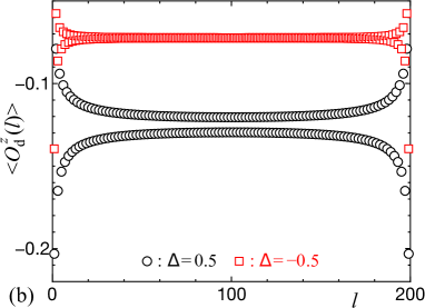
Figure 1: Expectation values of the dimer operators (a) $\langle\mathcal{O}_{\rm d}^{\pm}(l)\rangle$ and (b) $\langle\mathcal{O}_{\rm d}^{z}(l)\rangle$ in the ground state of the XXZ chain (1) for $\Delta=0.5,-0.5$, zero magnetic field $h=0$, and $L=200$.

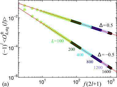
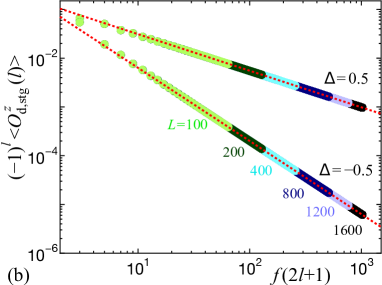
Figure 2: Staggered part of the expectation value of the dimer operators (a) $(-1)^{l}\langle\mathcal{O}_{\rm d,stg}^{\pm}(l)\rangle$ and (b) $(-1)^{l}\langle\mathcal{O}_{\rm d,stg}^{z}(l)\rangle$ in the ground state of the XXZ chain (1) for $\Delta=0.5,-0.5$ and zero magnetic field $h=0$. The data for $L=100,200,400,800,1200$, and $1600$ are plotted. The dashed lines represent the expected behavior, $c_{1}^{a}/[f(2l+1)]^{1/2\eta}$, with $c_{1}^{a}$ obtained by the procedure explained in the text and $\eta$ given by Eq. (3).

In order to estimate the coefficients $c_{1}^{a}$ ($a=\pm,z$) for the XXZ chain at zero field, we computed the ground-state expectation values of the dimer operators, $\langle\mathcal{O}_{\rm d}^{a}(l)\rangle$, for the systems up to $L=1600$ spins. Figure 1 shows the numerical results for $\Delta=0.5$ and $\Delta=-0.5$. (Here we plot the results obtained for a rather small system size $L=200$ for clarity.) The ground-state expectation values of the dimer operators exhibit sizable Friedel oscillations near open boundaries. The staggered part of the expectation values of the dimer operators, $\langle\mathcal{O}_{\rm d,stg}^{a}(l)\rangle$, can be obtained from $\langle\mathcal{O}_{\rm d}^{a}(l)\rangle$ by subtracting the non-oscillating contributions,

$$\langle\mathcal{O}_{\rm d,stg}^{a}(l)\rangle=\langle\mathcal{O}_{\rm d}^{a}(l)\rangle-c_{0}^{a}+\frac{\pi^{2}c_{2}^{a}}{12(L+1)^{2}}+\frac{\bar{c}_{2}^{a}}{[f(2l+1)]^{2}},$$ (28)

where the exact values given in Eqs. (11) and (25) are substituted for the coefficients $c_{0}^{a}$, $c_{2}^{a}$, and $\bar{c}_{2}^{a}$. The staggered part $\langle\mathcal{O}_{\rm d,stg}^{a}(l)\rangle$ obtained in this way is shown in Fig. 2. We see that data points of $(-1)^{l}\langle\mathcal{O}_{\rm d,stg}^{a}(l)\rangle$ computed for different system sizes collapse onto a single line in the log-log plot, which corresponds to the power-law behavior $(-1)^{l}\langle\mathcal{O}_{\rm d,stg}^{a}(l)\rangle=c_{1}^{a}/[f(2l+1)]^{1/2\eta}$. This demonstrates the validity of Eq. (23) and indicates that the higher-order terms neglected there are indeed very small.

The coefficients $c_{1}^{a}$ are obtained from $\langle\mathcal{O}_{\rm d,stg}^{a}(l)\rangle$ as follows. For an open spin chain of $L$ sites, we calculate

$$c_{1}^{a}(l,L)=(-1)^{l}\langle\mathcal{O}_{\rm d,stg}^{a}(l)\rangle[f(2l+1)]^{1/2\eta}$$ (29)

for each $l$ in the central region ($L/2-10\leq l\leq L/2+10$) and the spatial average of $c_{1}^{a}(l,L)$ over the central region is denoted by $c_{1}^{a}(L)$. We calculate $c_{1}^{a}(L)$ for several values of $L$ and obtain a set of data $\mathcal{C}_{1}^{a}=\{c_{1}^{a}(L)|L=100,200,\ldots,1600\}$. For three different subsets of $\mathcal{C}_{1}^{a}$ we fit $c_{1}^{a}(L)$ to the polynomial $c_{1}^{a}(L)=c_{1}^{a}(\infty)+\beta_{1}^{a}/L+\beta_{2}^{a}/L^{2}$; this defines the extrapolated value $c_{1}^{a}(\infty)$ for each subset of $\mathcal{C}_{1}^{a}$. We take the average of these $c_{1}^{a}(\infty)$ as the final estimate of $c_{1}^{a}$. The error is determined from the largest of the differences of the final estimate $c_{1}^{a}$ from the extrapolated values $c_{1}^{a}(\infty)$ for the subsets of $\mathcal{C}_{1}^{a}$ and from the estimates $c_{1}^{a}(l,L)$ for the central region of the largest system $L=1600$. In this way we have determined the coefficients $c_{1}^{a}$ for $\Delta\geq-0.6$, but we could not obtain accurate results for $\Delta\leq-0.7$, where the Friedel oscillations in $\langle\mathcal{O}_{\rm d}^{a}(l)\rangle$ decay so rapidly that the amplitude of oscillations away from the boundaries becomes almost comparable to the numerical accuracy of our DMRG data. The results for the amplitudes $B_{1}^{a}=(c_{1}^{a})^{2}/2$ of the leading staggered term of the dimer correlation functions are presented in Table 1 and Fig. 3.

Figure 3: Amplitudes $B_{1}^{a}=(c_{1}^{a})^{2}/2$ of the leading staggered term in the dimer correlation functions, Eq. (5), in the XXZ chain (1) at zero magnetic field $h=0$.

Table 1: Amplitudes $B_{1}^{a}=(c_{1}^{a})^{2}/2$ of the leading staggered term in the dimer correlation functions (5) in the XXZ chain (1) for $h=0$ as functions of the anisotropy parameter $\Delta$. The number in the parentheses for the value of $B_{1}^{a}$ denotes the error in the last digit. The error was estimated as described below Eq. (29).systematic_error

$\Delta$	$B_{1}^{\pm}$	$B_{1}^{z}$
0.9	0.00582(6)	0.00606(7)
0.8	0.00826	0.00898
0.7	0.01008(2)	0.01144(2)
0.6	0.01139(2)	0.01351(3)
0.5	0.01229(2)	0.01528(3)
0.4	0.01285(1)	0.01677(2)
0.3	0.01314(1)	0.01804(1)
0.2	0.01319(1)	0.01909(1)
0.1	0.01302(1)	0.01992(2)
0.0	0.01267(1)	0.02055(2)
$-0.1$	0.01216(1)	0.02095(2)
$-0.2$	0.01149(1)	0.02112(2)
$-0.3$	0.01068(1)	0.02103(2)
$-0.4$	0.00975(1)	0.02066(2)
$-0.5$	0.00872(1)	0.01999(3)
$-0.6$	0.00760(7)	0.0190(3)

II.3 Application

The high-precision data of the coefficients $c_{1}^{a}$ can be used for quantitative analysis of physical quantities related to the dimer operators, including spin-Peierls instability, dynamical structure factors of dimer correlations, and interchain dimer-dimer couplings in quasi-1D systems. As an example of such applications, we discuss the excitation gap in the XXZ chain with bond alternation in this section.

Let us consider the bond-alternating spin-1/2 XXZ chain, whose Hamiltonian is

$$\mathcal{H}_{\rm ba}=J\sum_{l=1}^{L-1}\left[1-(-1)^{l}\delta\right]\!(S^{x}_{l}S^{x}_{l+1}+S^{y}_{l}S^{y}_{l+1}+\Delta S^{z}_{l}S^{z}_{l+1}),$$ (30)

where $\delta$ is a positive parameter controlling the magnitude of the bond alternation. We assume the easy-plane anisotropy, $|\Delta|<1$. From Eq. (8), it is found that the low-energy effective Hamiltonian for Eq. (30) is given by

$$\widetilde{\mathcal{H}}_{\rm ba}=\widetilde{\mathcal{H}}_{0}-J\delta\!\left(2c_{1}^{\pm}+\Delta c_{1}^{z}\right)\!\int\!dx\cos[\sqrt{2\pi}\phi(x)]+\cdots,$$ (31)

where $\widetilde{\mathcal{H}}_{0}$ is the Gaussian model in Eq. (6). Since the nonlinear term $\cos[\sqrt{2\pi}\phi(x)]$ has a scaling dimension $1/(2\eta)$ at the Gaussian fixed point, it is a relevant perturbation and opens an excitation gap if $\eta>1/4$ (i.e., $\Delta>-1/\sqrt{2}$). In this case the excitation gap $E_{\rm g}(\delta)$ for small bond alternation $\delta\ll 1$ is given byZamolodchikov1995

$$\frac{E_{\rm g}(\delta)}{J}=A(\Delta)\!\left|\delta(2c_{1}^{\pm}+\Delta c_{1}^{z})\right|^{2\eta/(4\eta-1)}$$ (32)

with

$$A(\Delta)=\frac{2v}{\sqrt{\pi}J}\frac{\Gamma\bigl{(}\frac{1}{8\eta-2}\bigr{)}}{\Gamma\bigl{(}\frac{2\eta}{4\eta-1}\bigr{)}}\!\left[\frac{\pi J}{2v}\frac{\Gamma\bigl{(}1-\frac{1}{4\eta}\bigr{)}}{\Gamma\bigl{(}\frac{1}{4\eta}\bigr{)}}\right]^{2\eta/(4\eta-1)}.$$ (33)

Note that the parameter $\eta$ and the spin velocity $v$ are functions of $\Delta$ [see Eqs. (3) and (7)]. Thus, with the estimates of $c_{1}^{a}$ obtained in Sec. II.2, we can determine the excitation gap from Eqs. (32) and (33) without any free parameter.

To confirm this theory, we numerically calculated the excitation gap $E_{\rm g}(\delta)$ for $\Delta=0.5$ and $\delta=2^{-3},...,2^{-10}$ using the DMRG method. The gap $E_{\rm g}(\delta)$ was obtained as follows. We first calculated the excitation gap for finite open spin chains of various lengths up to $L=3200$, using the relation

$$E_{\rm g}(\delta,L)=E_{0}(\delta;L,1)-E_{0}(\delta;L,0),$$ (34)

where $E_{0}(\delta;L,S^{z}_{\rm tot})$ is the lowest energy in the subspace in which the total magnetization $\sum_{l}S^{z}_{l}=S^{z}_{\rm tot}$. We thus obtained a set of data $\mathcal{E}=\{E_{\rm g}(\delta,L)|L=100,200,\ldots,3200\}$. For three different subsets of $\mathcal{E}$ we fit $E_{\rm g}(\delta,L)$ to a second-order polynomial, $E_{\rm g}(\delta,L)=E_{\rm g}(\delta,\infty)+\beta_{1}/L+\beta_{2}/L^{2}$, to obtain the extrapolated value $E_{\rm g}(\delta,\infty)$ for each subset of $\mathcal{E}$. We took the average of $E_{\rm g}(\delta,\infty)$ for the subsets as the final estimate of $E_{\rm g}(\delta)$. The error in $E_{\rm g}(\delta)$, which is estimated from the difference between the final estimate $E_{\rm g}(\delta)$ and the extrapolation $E_{\rm g}(\delta,\infty)$ for the subsets of $\mathcal{E}$, is less than $3.9\times 10^{-5}J$.

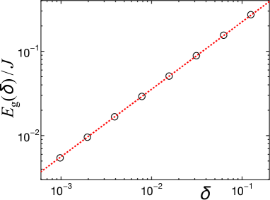
Figure 4: Excitation gap $E_{\rm g}(\delta)$ in the bond-alternating XXZ chain (30) at $\Delta=0.5$. The circles represent the gap $E_{\rm g}(\delta)$ obtained using the DMRG method and the extrapolation as described below Eq. (34). The dotted line shows the theoretical curve from Eqs. (32) and (33), in which the exact values of $\eta$ and $v$ [Eqs. (3) and (7)] and the coefficients $c_{1}^{\pm}$ and $c_{1}^{z}$ obtained in Sec. II.2 are substituted.

In Fig. 4, we show $E_{\mathrm{g}}(\delta)$, together with a plot of Eq. (32) calculated with $c_{1}^{a}$ obtained in the previous section. Clearly, the numerical and analytic results are in excellent agreement,diff_gap_d05 demonstrating the accuracy of the estimates of $c_{1}^{a}$ and the validity of the theory.

III SU(2) symmetric case

In this section we discuss the SU(2) symmetric case where $\Delta=1$ and $h=0$ in Eq. (1). In this case the marginally irrelevant operator in the low-energy effective theory brings about logarithmic corrections in various physical quantities.Giamarchi-text ; GogolinNT-text ; Affleck-text ; Lukyanov1998 ; VekuaS2016 ; Affleck1998 For example, the leading behavior of the dimer correlation function is

$$\langle\mathcal{O}_{\mathrm{d}}^{a}(l)\mathcal{O}_{\mathrm{d}}^{a}(l+r)\rangle-\langle\mathcal{O}_{\mathrm{d}}^{a}(l)\rangle\langle\mathcal{O}_{\mathrm{d}}^{a}(l+r)\rangle$$

$$~{}~{}~{}~{}~{}~{}~{}~{}=\widetilde{B}_{1}\frac{(-1)^{r}}{r\,(\ln r)^{3/2}}+\cdots,$$ (35)

for $r\gg 1$, where $\widetilde{B}_{1}$ is a constant common to $a=\pm,z$. This behavior can be understood within the scheme of the previous section as follows; in the SU(2) symmetric limit, the correlation amplitude $B_{1}=(c_{1})^{2}/2$ is renormalized and acquires logarithmic dependence on the length or energy scale of interest. Namely, $B_{1}\propto(\ln r)^{-3/2}$ and $c_{1}\propto(\ln r)^{-3/4}$. In the following, we reversely employ the analysis of Sec. II.3; that is, we deduce the amplitude $\widetilde{B}_{1}$ from the dependence of the excitation gap $E_{\mathrm{g}}$ on the bond alternation $\delta$.

Let us consider the Heisenberg spin chain with the bond alternation [Eq. (30) with $\Delta=1$]. The low-energy effective Hamiltonian is written in terms of the bosonic fields as

$$\widetilde{\mathcal{H}}_{\rm ba,SU(2)}= \,\widetilde{\mathcal{H}}_{0}-3c_{1}\delta J\int dx\cos[\sqrt{2\pi}\phi(x)]$$

$$+g\int dx\cos[\sqrt{8\pi}\phi(x)]+\cdots,$$ (36)

where $\widetilde{\mathcal{H}}_{0}$ is the Gaussian model in Eq. (6) and $c_{1}=c_{1}^{\pm}=c_{1}^{z}$. It is important to note that we have included the marginally irrelevant term, $g\int dx\cos[\sqrt{8\pi}\phi(x)]$, in the effective Hamiltonian. In the absence of the bond alternation ($\delta=0$), the coupling constant $g$ is renormalized to zero as $g\sim[\ln(J/E)]^{-1}$ with decreasing energy scale $E$. When the bond alternation is present, $\delta\neq 0$, the renormalization of the coupling constant $g$ is stopped at the energy scale of the excitation gap $E_{\rm g}$, where $g$ takes a finite value. Using the renormalization-group scheme from Ref. Lukyanov1998, , the relation between the gap $E_{\mathrm{g}}$ and the running coupling constant $g$ can be chosen as

$$\frac{E_{\rm g}}{J}=\sqrt{2\pi^{3}}\,e^{\gamma_{\rm E}}g^{-1/2}e^{-1/g},$$ (37)

where $\gamma_{\rm E}\simeq 0.5772...$ is the Euler constant.

We suppose that the gap formula of Eqs. (32) and (33) holds also in the SU(2) symmetric case and that logarithmic corrections manifest themselves through the renormalized coefficient $c_{1}$. Thus, we substitute $\eta=1$ and $v=\pi J/2$, which are the fixed-point values in the SU(2) case in the absence of the bond alternation, into Eqs. (32) and (33). Then we write

$$c_{1}=\frac{1}{(2\pi^{3})^{1/4}}\frac{g^{3/4}}{C(g)},$$ (38)

where

$$C(g)=(2\pi^{3})^{-1/4}g^{3/4}\frac{3\delta\Gamma\left(\frac{3}{4}\right)}{\Gamma\left(\frac{1}{4}\right)}\!\left[\frac{\Gamma\left(\frac{2}{3}\right)}{\sqrt{\pi}\,\Gamma\left(\frac{1}{6}\right)}\frac{E_{\rm g}}{J}\right]^{-3/2}.$$ (39)

We have defined $C(g)$ in such a way that the prefactor $g^{3/4}$ in Eq. (38) incorporates the scaling $c_{1}\propto g^{3/4}$ at $g\ll 1$. It is then natural to expect that $C(g)$ should be expanded in powers of $g$,

$$C(g)=C_{0}+C_{1}g+C_{2}g^{2}+\cdots$$ (40)

for $g\ll 1$.

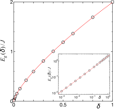
Figure 5: Excitation gap $E_{\rm g}(\delta)$ in the bond-alternating Heisenberg chain, Eq. (30) with $\Delta=1$. The circles represent the numerical data extrapolated to the thermodynamic limit $L\to\infty$, and the square is the exact value $E_{\rm g}(\delta=1)=2$. The red dotted line is the theoretical curve, Eqs. (37) and (41), with $C_{2}=1.80$. The inset shows the same figure in a log-log scale.

In order to estimate the constants $C_{0}$, $C_{1}$, and $C_{2}$ in Eq. (40), we calculated numerically the excitation gap $E_{\rm g}(\delta)$ in the bond-alternating chain (30) with $\Delta=1$ and $\delta=2^{-10},...,2^{-3},0.2,...,0.8$ using the DMRG method. Previous works have obtained the excitation gap $E_{\rm g}(\delta,L)$ for $L\lesssim 200$ spins.PapenbrockBDSS2003 ; KumarRSS2007 Here, we computed $E_{\rm g}(\delta,L)$ for the finite open chains up to $L\leq 3200$ ($L\leq 800$) spins with $2^{-10}\leq\delta\leq 2^{-3}$ ($0.2\leq\delta\leq 0.8$). We then extrapolated the data to $L\to\infty$ in the same manner as in Sec. II.3 and obtained the estimate of the gap $E_{\rm g}(\delta)$ in the thermodynamic limit. The error in $E_{\rm g}(\delta)$ is estimated to be less than $1.5\times 10^{-5}J$. The numerical results for $E_{\rm g}(\delta)$ are shown by open circles in Fig. 5.

Having determined $E_{\mathrm{g}}(\delta)$ numerically, we use Eq. (37) to obtain the renormalized coupling constant $g$ as a function of $\delta$. Then we substitute $E_{\mathrm{g}}(\delta)$ and $g(\delta)$ into the right-hand side of Eq. (39) to obtain $C(g)$ for each $\delta$ calculated. In Fig. 6, we plot the so-obtained $C(g)$ (open circles). As clearly shown in Fig. 6, when plotted as a function of $g^{2}$, $C(g)$ exhibits a linear behavior and approaches unity as $g^{2}\to 0$. Fitting $C(g)$ of the $n$-smallest $g$ ($n=4-8$) to Eq. (40) while assuming $C_{1}=0$ and neglecting the higher-order terms $\mathcal{O}(g^{3})$, we obtain $0.995\leq C_{0}\leq 0.998$. These results indicate that $C_{0}=1$ and $C_{1}=0$. Then fitting $C(g)$ while assuming $C_{0}=1$ and $C_{1}=0$ yields $C_{2}\simeq 1.80(3)$.

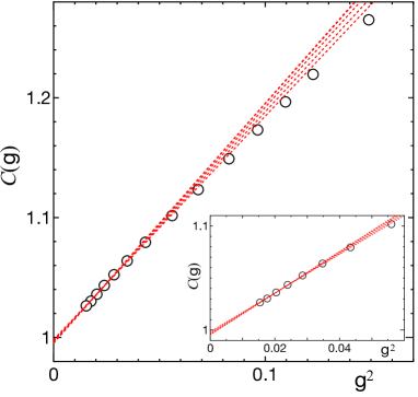
Figure 6: $C(g)$ as a function of $g^{2}$. The circles represent the numerical data. The red dotted lines show the fitting to $C(g)=C_{0}+C_{2}g^{2}$ of the data points at the $n$ smallest $g$ ($n=4,5,...,8$). The inset shows the same figure on an enlarged scale.

The results obtained above lead to the following expression for the excitation gap. From Eqs. (39) and (40), we can write the bond alternation $\delta$ in terms of $E_{\rm g}$ and $g$ as

$$\delta=\frac{2\Gamma\left(\frac{1}{4}\right)}{3\Gamma\left(\frac{3}{4}\right)}\!\left[\frac{\Gamma\left(\frac{2}{3}\right)}{\sqrt{2}\Gamma\left(\frac{1}{6}\right)}\frac{E_{\rm g}}{J}\right]^{3/2}g^{-3/4}\bigl{(}1+C_{2}g^{2}\bigr{)},$$ (41)

where we have substituted $C_{0}=1$ and $C_{1}=0$ in Eq. (40) and omitted the higher-order terms $\mathcal{O}(g^{3})$ in $C(g)$. Equations (37) and (41) give a parametric representation of $E_{\rm g}(\delta)$ in terms of $g$. In Fig. 5, we plot the gap $E_{\rm g}(\delta)$ calculated from Eqs. (37) and (41). Clearly, the theoretical curve reproduces the numerical data. We emphasize that the agreement between the theory and numerical data is excellent even at the large bond alternation, $\delta\to 1$, suggesting that the effect of the higher-order terms $\mathcal{O}(g^{3})$ in $C(g)$ on the excitation gap $E_{\rm g}(\delta)$ is negligible. Our theory with Eqs. (37) and (41) thereby provides accurate values of $E_{\rm g}(\delta)$ for the whole range of the bond alternation $0<\delta\leq 1$.

In addition, the above theory allows us to derive the long-distance behavior of the dimer correlation function in the uniform Heisenberg chain [Eq. (1) with $\Delta=1$] in zero field $h=0$. Substituting Eq. (38) with $C(g)=1$ into Eq. (5) with $B_{1}^{a}=(c_{1}^{a})^{2}/2$ and replacing $g$ by $(\ln r)^{-1}$, we obtain

$$\langle\mathcal{O}_{\rm d}^{a}(l)\mathcal{O}_{\rm d}^{a}(l+r)\rangle-\langle\mathcal{O}_{\rm d}^{a}(l)\rangle\langle\mathcal{O}_{\rm d}^{a}(l+r)\rangle$$

$$~{}~{}~{}~{}~{}~{}~{}~{}=\frac{1}{(2\pi)^{3/2}}\frac{(-1)^{r}}{r\,(\ln r)^{3/2}}+\cdots,$$ (42)

where $a=\pm,z$ (no summation is taken for the repeated index $a$). Note that the correlation functions of $\mathcal{O}_{\rm d}^{\pm}$ and $\mathcal{O}_{\rm d}^{z}$ are identical due to the SU(2) symmetry. We note that the amplitude $\widetilde{B}_{1}=(2\pi)^{-3/2}=0.0635...$ is in good agreement with the recent numerical estimate $0.067$ reported in Ref. VekuaS2016, .

IV XXZ chain with nonzero magnetization

IV.1 Theory

In this section, we study the XXZ chain (1) in the TLL phase with a partial spin polarization under finite external field $h_{\rm c}<h<h_{\rm s}$. Here, $h_{\rm c}$ is the lower critical field ($h_{\rm c}=0$ for $-1<\Delta\leq 1$ and $h_{\rm c}>0$ for $\Delta>1$), while $h_{\rm s}=J(1+\Delta)$ is the saturation field. The low-energy effective theory in this case is the Gaussian model (6) again. In the partially polarized state with $0<M<1/2$, the Fermi momentum $k_{\rm F}$ of the Jordan-Wigner fermions is shifted from the commensurate value $k_{\rm F}=\pi/2$ at $M=0$ to the incommensurate one $k_{\rm F}=\pi(\frac{1}{2}+M)$. The boson-field expression of the dimer operator (4) is then modified from Eq. (8) into

$$\mathcal{O}_{\rm d}^{a}(l)= \,c_{0}^{a}+c_{1}^{a}(-1)^{l}\cos[Qx_{l}+\sqrt{2\pi}\phi(x_{l})]$$

$$+c_{\phi}^{a}\left(\frac{d\phi(x_{l})}{dx}\right)^{2}+c_{\theta}^{a}\left(\frac{d\theta(x_{l})}{dx}\right)^{2}$$

$$+c_{g}^{a}\cos[2Qx_{l}+\sqrt{8\pi}\phi(x_{l})]+\cdots$$ (43)

for $a=\pm,z$. The wave number $Q$ of the leading oscillating term is $Q=2\pi M$ in the limit $L\to\infty$.

In the same manner as in Sec. II.1, we can calculate the ground-state expectation values of the dimer operators in Eq. (4) in finite chains with open boundaries. For the partially polarized state, we find it necessary to optimize the positions at which the Dirichlet boundary condition is imposed, in order to achieve a better fitting of the numerical data.Fath2003 ; HikiharaMFK2010 We thus employ the Dirichlet boundary conditions $\phi(x_{0})=\phi(L+1-x_{0})=0$, instead of Eq. (17). Accordingly, the one-point functions of the dimer operators become

$$\langle\mathcal{O}_{\rm d}^{a}(l)\rangle= \,c_{0}^{a}+\frac{c_{1}^{a}(-1)^{l}\cos[\tilde{Q}(l+1/2-x_{0})]}{[\tilde{f}(2l+1-2x_{0})]^{1/2\eta}}$$

$$-\frac{\pi^{2}c_{2}^{a}}{12(L+1-2x_{0})^{2}}-\frac{\bar{c}_{2}^{a}}{[\tilde{f}(2l+1-2x_{0})]^{2}}$$

$$+\frac{c_{g}^{a}\cos[2\tilde{Q}(l+1/2-x_{0})]}{[\tilde{f}(2l+1-2x_{0})]^{2/\eta}}+\cdots,$$ (44)

where $\tilde{Q}=2\pi ML/(L+1-2x_{0})$ and

$$\tilde{f}(x)=\frac{2(L+1-2x_{0})}{\pi}\sin\!\left(\frac{\pi|x|}{2(L+1-2x_{0})}\right).$$ (45)

The parameter $\eta$ can be determined exactly by solving the integral equations obtained from the Bethe ansatz.BogoliubovIK1986 ; QinFYOA1997 ; CabraHP1998 We have kept the last term ($\propto c_{g}^{a}$) in Eq. (44) since it becomes larger than the third and fourth terms for $\eta>1$, which realizes at $\Delta>1$ and not too large $M>0$.

The coefficients of the uniform parts, $c_{0}^{a}$, $c_{2}^{a}$, $\bar{c}_{2}^{a}$, and $c_{g}^{a}$, are related to the ground-state energy density $e_{0}$, the spin velocity $v$, the exponent $\eta$, and the coupling constant $g$ through equations similar to Eqs. (9), (13), and (15), while explicit closed formulas for $e_{0}$, $v$, $\eta$, and $g$ are not available for $0<M<1/2$. On the other hand, the exact values of the coefficients $c_{1}^{a}$ of the oscillating terms are not known except for the free-fermion case $\Delta=0$,

$$c_{1}^{\pm}(\Delta=0) =\frac{1}{2\pi},$$ (46a)

$$c_{1}^{z}(\Delta=0) =\frac{2}{\pi^{2}}[\cos(\pi M)+\pi M\sin(\pi M)].$$ (46b)

We will determine the coefficients $c_{1}^{a}$ in the following numerical analysis.

IV.2 Numerical results

Using the DMRG method, we calculated the expectation values of the dimer operators $\langle\mathcal{O}_{\rm d}^{a}(l)\rangle$ in the partially-polarized ground state of the XXZ chain (1) with $L=100,200$, and $400$ spins for fixed magnetization $M$. We then fit the data to the analytic form (44) by taking $c_{1}^{a}$, $\bar{c}_{2}^{a}$, $c_{g}^{a}$, $c_{u}^{a}:=c_{0}^{a}-\pi^{2}c_{2}^{a}/[12(L+1-2x_{0})^{2}]$, and $x_{0}$ as fitting parameters.optimized_x0 The exponent $\eta$ was obtained from the Bethe ansatz integral equations.

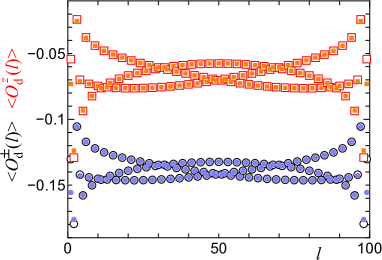
Figure 7: Expectation values of the dimer operators in the ground state of the XXZ chain (1) for $\Delta=0.5$, $M=0.16$, and $L=100$. The circles and squares correspond to $\langle\mathcal{O}_{\rm d}^{\pm}(l)\rangle$ and $\langle\mathcal{O}_{\rm d}^{z}(l)\rangle$, respectively. The open and solid symbols represent the DMRG data and the fitting results, respectively.

We show in Fig. 7 the DMRG data and the fitting results for $\Delta=0.5$ and $M=0.16$. (The data for the small system $L=100$ are shown for clarity.) The agreement between the DMRG data and the fits is excellent, which demonstrates the validity of Eq. (44) and justifies our scheme for estimating $c_{1}^{a}$.

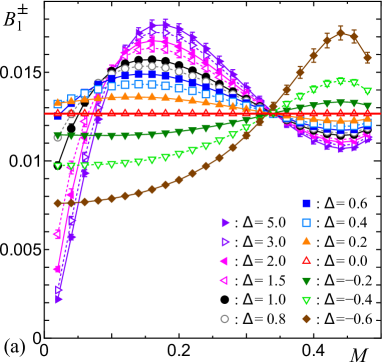
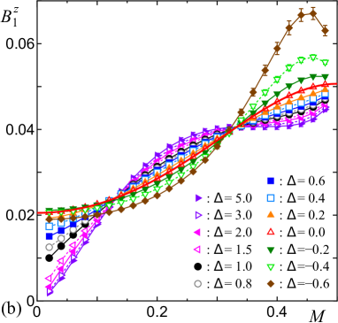
Figure 8: Amplitudes $B_{1}^{a}=(c_{1}^{a})^{2}/2$ of the leading oscillating term in the dimer correlation functions in Eq. (5) as functions of $M$ for various values of the anisotropy parameter $\Delta$: (a) $B_{1}^{\pm}$ and (b) $B_{1}^{z}$. The thick lines represent the exact results for $\Delta=0$, Eq. (46). The thin lines are guides for the eye.

For each system size $L$, we fit the numerical data of $\langle\mathcal{O}_{\rm d}^{a}(l)\rangle$ in three different ranges of $l$ to estimate the coefficients $c_{1}^{a}$ ($a=\pm,z$), which we denote $c_{1}^{a}(i,L)$ ($i=1,2,3$), and took their averages as the estimate $c_{1}^{a}(L)$ for the system size $L$. Then, we extrapolated the results for $L=100,200,$ and $400$ by fitting them to the polynomial form $c_{1}^{a}(L)=c_{1}^{a}(\infty)+\beta_{1}^{a}/L$ and took the extrapolated value $c_{1}^{a}(\infty)$ as the final estimate of $c_{1}^{a}$. The error was determined from the differences between the final estimate and the estimates $c_{1}^{a}(i,L)$ at $L=400$. Figure 8 shows the so-obtained values of the amplitudes $B_{1}^{a}=(c_{1}^{a})^{2}/2$ of the dimer correlation functions in Eq. (5). We note that the numerical estimates for the free-fermion case ($\Delta=0$) agree with the exact values in Eq. (46). Figure 8 also indicates that in the saturation limit $M\to 1/2$, the amplitudes converge at universal values, $B_{1}^{\pm}=1/(8\pi^{2})$ and $B_{1}^{z}=1/(2\pi^{2})$. This behavior is easily understood as the $\Delta S^{z}_{l}S^{z}_{l+1}$ interactions between magnons are not effective in the limit of dilute magnon density, $M\to 1/2$. The numerical data of the amplitudes $B_{1}^{a}$ are presented in the Supplemental Material.supplement

Another interesting feature found in Fig. 8 is that the curves of $B_{1}^{a}$ for different values of $\Delta$ seem to intersect at an intermediate value of magnetization, $M\simeq 0.33-0.34$. Interestingly enough, the amplitude $A_{1}^{z}$ of the longitudinal spin-spin correlation function $\langle S^{z}_{l}S^{z}_{l+r}\rangle$ [Eq. (LABEL:eq:SzSzcor)] is also foundHikiharaF2004 to exhibit a similar behavior of intersection of $\Delta$-dependent curves at $M\simeq 0.365$ [see Fig. 2(c) in Ref. HikiharaF2004, ]. At present, we do not know exactly whether and why these correlation amplitudes really become independent of $\Delta$ at some intermediate $M$. Furthermore, it is not clear whether or not the values of $M$ at which $B_{1}^{a}$ and $A_{1}^{z}$ become independent of $\Delta$ are the same. These questions are open for future studies.

V Conclusion

We have studied the dimer correlation functions in the ground state of the spin-1/2 XXZ chain in the critical Tomonaga-Luttinger-liquid regime. We have determined with high accuracy the amplitudes of the leading oscillating terms of the dimer correlation functions in the XXZ chain for both zero and finite magnetic fields, using the bosonization and DMRG methods. We have also investigated the dimer correlations and the spin-Peierls instability in the SU(2) symmetric chain (i.e., the antiferromagnetic Heisenberg model in zero field), in which the marginally-irrelevant operator in the low-energy effective Hamiltonian yields logarithmic corrections. We have derived the asymptotic formula for the excitation gap in the SU(2) symmetric chain with bond alternation and numerically determined the coefficients of the first few terms in the formula expanded in powers of the coupling constant. From the formula of the gap, we have obtained the asymptotic power-law behavior of the dimer correlation function with a multiplicative logarithmic correction, Eq. (42).

The dimer correlation amplitudes obtained in this work can be used for quantitative study of physical properties related to the dimer operators, such as the spin-Peierls instability, dynamical structure factors of dimer operators measured in resonant inelastic x-ray scattering experiments, the effects of weak interchain dimer-dimer interactions in quasi-1D systems, etc.

- (1) T. Giamarchi, Quantum Physics in One Dimension (Oxford University Press, New York,2004).
- (2) A. O. Gogolin, A. A. Nersesyan, and A. M. Tsvelik, Bosonization and Strongly Correlated Systems (Cambridge University Press, 1998).
- (3) I. Affleck, in Fields, Strings and Critical Phenomena (Les Houches 1988, Session 49), edited by E. Brézin and J. Zinn-Justin, (North-Holland, Amsterdam, 1990), p. 563.
- (4) A. Luther and I. Peschel, Phys. Rev. B 12, 3908 (1975).
- (5) S. Lukyanov and A. Zamolodchikov, Nucl. Phys. B 493, 571 (1997).
- (6) S. Lukyanov, Nucl. Phys. B 522, 533 (1998).
- (7) S. Lukyanov, Phys. Rev. B 59, 11163 (1999).
- (8) S. Lukyanov and V. Terras, Nucl. Phys. B 654, 323 (2003).
- (9) T. Hikihara and A. Furusaki, Phys. Rev. B 58, R583 (1998).
- (10) T. Hikihara and A. Furusaki, Phys. Rev. B 63, 134438 (2001).
- (11) T. Hikihara and A. Furusaki, Phys. Rev. B 69, 064427 (2004).
- (12) A. Shashi, M. Panfil, J.-S. Caux, and A. Imambekov, Phys. Rev. B 85, 155136 (2012).
- (13) J.-S. Caux, H. Konno, M. Sorrell, and R. Weston, J. Stat. Mech. P01007 (2012).
- (14) M. C. Cross and D. S. Fisher, Phys. Rev. B 19, 402 (1979).
- (15) S. Takayoshi and M. Sato, Phys. Rev. B 82, 214420 (2010).
- (16) H. Suzuura, H. Yasuhara, A. Furusaki, N. Nagaosa, and Y. Tokura, Phys. Rev. Lett. 76, 2579 (1996).
- (17) L. J. P. Ament, M. van Veenendaal, T. P. Devereaux, J. P. Hill, and J. van den Brink, Rev. Mod. Phys. 83, 705 (2011).
- (18) T. Nagao and J. Igarashi, Phys. Rev. B 75, 214414 (2007).
- (19) A. Klauser, J. Mossel, J.-S. Caux, and J. van den Brink, Phys. Rev. Lett. 106, 157205 (2011).
- (20) A. Klauser, J. Mossel, and J.-S. Caux, J. Stat. Mech. P03012 (2012).
- (21) T. Vekua and G. Sun, Phys. Rev. B 94, 014417 (2016).
- (22) J. des Cloizeaux and J. J. Pearson, Phys. Rev. 128, 2131 (1962).
- (23) N. M. Bogoliubov, A. G. Izergin, and V. E. Korepin, Nucl. Phys. B 275, 687 (1986).
- (24) C. N. Yang and C. P. Yang, Phys. Rev. 150, 321 (1966).
- (25) C. N. Yang and C. P. Yang, Phys. Rev. 150, 327 (1966).
- (26) R. J. Baxter, Ann. Phys. 70, 323 (1972).
- (27) A. Furusaki and T. Hikihara, Phys. Rev. B 69, 094429 (2004); 70, 189902(E) (2004).
- (28) S. Furukawa, M. Sato, and A. Furusaki, Phys. Rev. B 81, 094430 (2010).
- (29) S. Eggert and I. Affleck, Phys. Rev. B 46, 10866 (1992).
- (30) We note that the leading irrelevant operator is not included in the effective Hamiltonian (6) used in our analysis for . This may induce systematic errors for close to unity, in addition to the estimated numerical errors shown in the Table I. We expect that the extrapolation of to performed in our analysis should lessen potential systematic errors.
- (31) AL. B. Zamolodchikov, Int. J. Mod. Phys. A 10, 1125 (1995).
- (32) The relative difference between the DMRG data (circles) and the analytic results (dotted line) in Fig. 4 is about 1.2% at , 1.7% at , and smaller for intermediate values of . The difference at is on the same order as the numerical error in the DMRG data of .
- (33) I. Affleck, J. Phys. A: Math. Gen. 31, 4573 (1998).
- (34) T. Papenbrock, T. Barnes, D. J. Dean, M. V. Stoitsov, and M. R. Strayer, Phys. Rev. B 68, 024416 (2003).
- (35) M. Kumar, S. Ramasesha, D. Sen, and Z. G. Soos, Phys. Rev. B 75, 052404 (2007).
- (36) G. Fáth, Phys. Rev. B 68, 134445 (2003).
- (37) T. Hikihara, T. Momoi, A. Furusaki, and H. Kawamura, Phys. Rev. B 81, 224433 (2010).
- (38) S. Qin, M. Fabrizio, L. Yu, M. Oshikawa, and I. Affleck, Phys. Rev. B 56, 9766 (1997).
- (39) D. C. Cabra, A. Honecker, and P. Pujol, Phys. Rev. B 58, 6241 (1998).
- (40) The values of obtained from the fitting were typically small, , while took large negative values for strong Ising anisotropy (large ) and small , e.g., () for , , and ().
- (41) See Supplemental Material for the data for .