Irreversible mixing by unstable periodic orbits in buoyancy dominated stratified turbulence

Abstract

We consider turbulence driven by a large-scale horizontal shear in Kolmogorov flow (i.e. with sinusoidal body forcing) and a background linear stable stratification with buoyancy frequency $N_{B}^{2}$ imposed in the third, vertical direction in a fluid with kinematic viscosity $\nu$. This flow is known to be organised into layers by nonlinear unstable steady states, which incline the background shear in the vertical and can be demonstrated to be the finite-amplitude saturation of a sequence of instabilities, originally from the laminar state. Here, we investigate the next order of motions in this system, i.e. the time-dependent mechanisms by which the density field is irreversibly mixed. This investigation is achieved using ‘recurrent flow analysis’. We identify (unstable) periodic orbits, which are embedded in the turbulent attractor, and use these orbits as proxies for the chaotic flow. We find that the time average of an appropriate measure of the ‘mixing efficiency’ of the flow $\mathscr{E}=\chi/(\chi+\mathcal{D})$ ($\mathcal{D}$ is the volume-averaged kinetic energy dissipation rate and $\chi$ is the volume-averaged density variance dissipation rate) varies non-monotonically with the time-averaged buoyancy Reynolds numbers $\overline{Re}_{B}=\overline{\mathcal{D}}/(\nu N_{B}^{2})$, and is bounded above by $1/6$, consistently with the classical model of Osborn (1980). There are qualitatively different physical properties between the unstable orbits that have lower irreversible mixing efficiency at low $\overline{Re}_{B}\sim O(1)$ and those with nearly optimal $\mathscr{E}\lesssim 1/6$ at intermediate $\overline{Re}_{B}\sim 10$. The weaker orbits, inevitably embedded in more strongly stratified flow, are characterised by straining or ‘scouring’ motions, while the more efficient orbits have clear overturning dynamics in more weakly stratified, and apparently shear-unstable flow.

1 Introduction

A fundamental outstanding problem in stratified turbulence relates to the mixing of the stratifying agent, e.g. heat or salinity. Moreover such flows typically exhibit strong anisotropy with vertical motions being suppressed due to gravitational forces, and layerwise motions commonly being observed. The route by which the flow field rearranges the density field into well-defined mixed regions or ‘layers’ separated by sharp gradients or ‘interfaces’ as well as the layer/interface structure’s robustness are subjects of continuing research. A widely utilised characterisation of mixing comes in the form of some appropriate measure of the ‘mixing efficiency’, often defined as the ratio of irreversible potential energy increase relative to the irreversible kinetic energy loss (Peltier & Caulfield, 2003). One reason for this interest in mixing efficiency stems from the effort to devise accurate parameterisations of diapycnal diffusivity for use in ocean models, and there is growing evidence that such parameterisations should take into account variation of the efficiency with control parameters (Salehipour et al., 2016; Mashayek et al., 2017).

Here our approach to explore mixing in a turbulent stratified (shear-driven) flow is somewhat unconventional; rather than a statistical examination of increasingly large simulations or high-fidelity experimental/field data, we consider flows from the perspective of a high dimensional dynamical system and look for representative unstable solutions embedded within the stratified turbulence. Such an approach has seen great success in clarifying the behaviour of transitional wall-bounded shear flows (Kawahara & Kida, 2001; Cvitanović & Gibson, 2010; Kawahara et al., 2012) as well as the sustaining mechanisms exhibited by stationary turbulence (van Veen et al., 2006; Chandler & Kerswell, 2013; Lucas & Kerswell, 2017). Recently Lucas et al. (2017), (henceforth LCK17) have shown how such an approach can advance our understanding of layer formation by locating nonlinear layered steady states about which the turbulence organises. Given this success, we are motivated to investigate whether the next order of motions can be identified, those time-dependent simple invariant manifolds, i.e. periodic orbits, which capture some salient signature of the processes by which buoyancy is mixed. In particular, we are interested in how ‘efficient’ (defined in a precise fashion below) such mixing is, and how such processes vary with control parameters.

To address these issues, the paper is organised as follows. Section 2 contains the formulation and discussion of the methods employed, while section 3 presents a set of preliminary and motivational direct numerical simulations (DNS) with a discussion of their mixing properties. Section 4 shows results from the recurrent flow analysis together with a discussion of the processes exhibited by the periodic orbits discovered, and finally section 5 presents our conclusions.

2 Formulation

We begin by considering the following version of the non-dimensionalised, monochromatic body-forced, incompressible, Boussinesq equations

$$\frac{\partial\bm{u}}{\partial t} +\bm{u}\cdot\nabla\bm{u}+\nabla p=\frac{1}{Re}\Delta\bm{u}+\sin(ny)\mathbf{\hat{x}}-B\rho\mathbf{\hat{z}},$$ (1)

$$\frac{\partial\rho}{\partial t} +\bm{u}\cdot\nabla\rho=w+\frac{1}{RePr}\Delta\rho,\qquad\qquad\nabla\cdot\bm{u}=0$$ (2)

where we define the (external) Reynolds number $Re$, the bulk stratification parameter $B$ and the Prandtl number $Pr$ as

$$Re:=\frac{\sqrt{\lambda}}{\nu}\left(\frac{L_{y}}{2\pi}\right)^{3/2},\quad B:=\frac{g\beta L_{y}^{2}}{\rho_{0}\lambda 4\pi^{2}},\qquad Pr=\frac{\nu}{\kappa}.$$ (3)

Here, $\bm{u}(x,y,z,t)=u\mathbf{\hat{x}}+v\mathbf{\hat{y}}+w\mathbf{\hat{z}}$ is the three-dimensional velocity field, $p$ is the pressure and the density is decomposed into $\rho_{tot}=\rho_{0}+\rho_{B}(z)+\rho(\bm{x},t)$, i.e as the sum of a Boussinesq reference density, a constant linear background stratification and a fully varying disturbance density. We have non-dimensionalised using the characteristic length scale $L_{y}/2\pi$, characteristic time scale $\sqrt{L_{y}/2\pi\lambda}$ and density gradient scale $\beta={\rm d}\rho^{*}_{B}/{\rm d}z.$ (see LCK17 for details). Furthermore, $n$ is the forcing wavenumber, $\lambda$ is the forcing amplitude, $\nu$ is the kinematic viscosity, $\kappa$ is the molecular diffusivity. We impose periodic boundary conditions in all directions and solve over the cuboid $[0,2\pi/\alpha]\times[0,2\pi]^{2}$ where $\alpha=L_{y}/L_{x}$ defines the horizontal aspect ratio of the domain. Vorticity $\bm{\omega}=\nabla\times\bm{u}$ is used as the prognostic variable and DNS are performed using the fully dealiased (two-thirds rule) pseudospectral method with mixed fourth order Runge-Kutta and Crank-Nicolson timestepping implemented in CUDA to run on GPU cards. We initialise the velocity field’s Fourier components with uniform amplitudes and randomised phases in the range $2.5\leq|\bm{k}|\leq 9.5$ such that the total enstrophy $\langle|\bm{\omega}|^{2}\rangle_{V}=1$ and $\rho^{\prime}=0$ initially. Throughout, $\langle(\cdot)\rangle_{V}:=\alpha\int\!\!\int\!\!\int(\cdot)\,dxdydz/(2\pi)^{3}$ denotes a volume average, $\langle(\cdot)\rangle_{h}:=\alpha\int\!\!\int(\cdot)\,dxdy/(2\pi)^{2}$ denotes a horizontal average and $\langle(\cdot)\rangle_{v}:=\int\!(\cdot)\,dz/(2\pi)$ denotes a vertical average.

We define the diagnostics involved in the energetic budgets as

$$\mathcal{K} =\frac{1}{2}\langle|\bm{u}|^{2}\rangle_{V},\quad\mathcal{P}=\frac{B}{2}\langle\rho^{2}\rangle_{V},\quad\mathcal{I}=\langle\bm{u}\cdot\bm{f}\rangle_{V}=\langle u\sin(ny)\rangle_{V},$$ (4)

$$\mathcal{B} =\langle\bm{u}\cdot B\rho\mathbf{\hat{z}}\rangle_{V}=B\langle w\rho\rangle_{V},\quad\mathcal{D}=\frac{1}{Re}\langle|\nabla\bm{u}|^{2}\rangle_{V},\quad\chi=\frac{B}{PrRe}\langle|\nabla\rho|^{2}\rangle_{V},$$ (5)

where $\frac{{\rm d}\mathcal{K}}{{\rm d}t}=\mathcal{I}-\mathcal{B}-\mathcal{D},\quad\frac{{\rm d}\mathcal{P}}{{\rm d}t}=\mathcal{B}-{\chi}$ and $\mathcal{K}$ is the total kinetic energy density, $\mathcal{P}$ the density variance, $\mathcal{I}$ is the energy input by the forcing, $\mathcal{B}$ is the buoyancy flux, $\mathcal{D}$ is the viscous dissipation rate, and $\chi$ the density variance dissipation rate. We fix $\alpha=0.5$ to avoid subcritical transition, $Pr=1$ for numerical efficiency and $n=1$, i.e. the flow is forced with $\sin(y)\mathbf{\hat{x}},$ to mimic closely other large scale shear profiles previously studied (e.g. stratified Taylor-Couette flow (Woods et al., 2010) and vertically sheared Kolmogorov flow (Garaud et al., 2015)) and denote time averages with overbars, i.e. $\overline{(\cdot)}=[\int_{0}^{T}(\cdot){\rm d}t]/T$ where $T$ is normally the full simulation time.

3 Irreversible mixing in the direct numerical simulations

We begin by characterising the mixing in this system by conducting a set of simulations across a range of $Re$ and $B.$ The pertinent single point diagnostics are presented in table 1. In particular we examine the irreversible mixing efficiency which we, following Salehipour & Peltier (2015) and Maffioli et al. (2016), define in terms of the dissipation rates:

$$\mathscr{E}(t)=\frac{\chi}{\chi+\mathcal{D}}.$$ (6)

The dependence of $\mathscr{E}$ on typical flow parameters is a crucial ongoing problem in stratified turbulence, and a source of some controversy. As discussed by Mater & Venayagamoorthy (2014), the flow of a turbulent, shear-driven stratified fluid has several competing time scales, and it is natural to attempt to parameterise $\mathscr{E}$ in terms of parameters quantifying the relative importance of these time scales. Using shear-instability simulations and comparison with observations, Salehipour et al. (2016) developed a parameterisation using two parameters: an appropriately defined ‘buoyancy Reynolds number’, effectively a ratio of the time scale of the stratification to the time scale of the turbulence; and an appropriately defined Richardson number, effectively a ratio of the square of the time scale of the vertical shear (assumed to be the dominant driver of the mixing) to the time scale of the stratification. In order to determine how the mixing efficiency varies with these dimensionless numbers in this flow, we define the buoyancy Reynolds number $Re_{B}(t)$ and the (local) gradient Richardson number $Ri_{G}(\bm{x},t)$ as (with the usual caveat that comparing different studies is difficult if the key parameters are defined differently)

$$Re_{B}(t) =\frac{\mathcal{D}Re}{B},\qquad Ri_{G}(\bm{x},t)=\frac{-B\frac{\partial\rho_{tot}}{\partial z}}{\left(\frac{\partial u_{h}}{\partial z}\right)^{2}},$$ (7)

where $(\partial u_{h}/\partial z)^{2}=(\partial u/\partial z)^{2}+(\partial v/\partial z)^{2}.$ $Ri_{G}$ is a pointwise quantity which characterises the relative stability of the flow to overturning shear instabilities, and developing an appropriate overall average for this quantity to characterise a particular flow should be performed with care, not least because locations of low vertical shear significantly skew the distributions of $Ri_{G}.$ The appropriate averaging used here is thus

$${Ri}_{B}(t)=\left\langle\frac{\left\langle-B\frac{\partial\rho_{tot}}{\partial z}\right\rangle_{h}}{\left\langle\left(\frac{\partial u_{h}}{\partial z}\right)^{2}\right\rangle_{h}}\right\rangle_{z}.$$ (8)

There are two important points to appreciate about these definitions. First, we have chosen to define $Ri_{B}$ with the total gradients of density while $Re_{B}$ only depends explicitly on the background $N_{B}.$ Second, although in principle these are independent nondimensional parameters, it remains to be established that they are in this flow, as there exist situations where they are strongly correlated (see e.g. Zhou et al. (2017)).

In figure 1(a) and (b) we plot the time-averaged mixing efficiency $\overline{\mathscr{E}}$ against the time-averaged parameters $\overline{Ri}_{B}$ and $\overline{Re}_{B}$. We observe non-monotonic dependence of $\overline{\mathscr{E}}$ on both parameters, in at least qualitative agreement with the experimental analysis of Linden (1979) and numerical simulations of Shih et al. (2005). Indeed, $\mathscr{E}$ appears to saturate near the critical value of $1/6$, (marked with a horizontal line) equivalent to the upper bound on the turbulent flux coefficient $\Gamma\simeq\mathscr{E}/(1-\mathscr{E})\leq 0.2$ proposed by Osborn (1980) and then decreases for $\overline{Re}_{B}\gtrsim 30,$ with a dependence not entirely unlike the $\overline{\mathscr{E}}\propto\overline{Re}_{B}^{-1/2}$ observed by Shih et al. (2005) in what they referred to as the ‘energetic’ regime (see Ivey et al. (2008) for a more detailed discussion).

However, although these similarities are intriguing, there are still significant differences. Firstly, we do not observe a ‘transitional’ plateau of approximately constant mixing efficiency at intermediate $\overline{Re}_{B}$. Indeed, the qualitative structure of the mixing efficiency curve is more reminiscent of the Padé approximant proposed by Mashayek et al. (2017) using (vertical) shear-instability numerical data as well as observations, where $\Gamma\propto Re_{B}^{1/2}$ and $Re_{B}^{-1/2}$ for small and large $Re_{B}$ respectively. Second, and once again reminiscent of the approach proposed by Mashayek et al. (2017) to parameterise mixing in terms of $\overline{Re}_{B}$ alone, the two parameters $\overline{Ri}_{B}$ and $\overline{Re}_{B}$ are actually closely correlated, and our simulations actually trace out a (monotonic) curve in $\overline{Ri}_{B}-\overline{Re}_{B}$ space, as shown in figure 1(c), independently of the externally imposed parameters $B$ and $Re$. The low mixing efficiency observed at high $\overline{Ri}_{B}$ can thus be understood as being entirely associated with weaker turbulence (smaller $\overline{Re}_{B}$) and the maximum mixing efficiency occurs at a sweet spot of sufficiently vigorous turbulence at sufficiently high stratification, analogously to the results of Zhou et al. (2017). We stress that we are not claiming that this clear correlation between $\overline{Ri}_{B}$ and $\overline{Re}_{B}$ is generic, (see for example the discussion in Scotti & White (2016)) just that it occurs for this flow.

It is apparent that at small $\overline{Ri}_{B}$, $\overline{Ri}_{B}\propto\overline{Re}_{B}^{-1}$. This is unsurprising, as the turbulence and shear are largely unaffected by such weak stratification, and the variation of both parameters with $B$ completely dominates. As $\overline{Ri}_{B}$ increases beyond the value associated with the most efficient mixing however, the turbulence and shear do indeed become suppressed by the strengthening stratification, and the power law dependence steepens so $\overline{Ri}_{B}\propto\overline{Re}_{B}^{-3/2}$. There is undoubtedly also an increasing significance of viscosity, which becomes dominant for the largest values of $\overline{Ri}_{B}>1$, where $\overline{Re}_{B}$ drops below one, and the turbulence is essentially completely suppressed, with very inefficient mixing. However, it is always important to remember that both $\overline{Ri}_{B}$ and $\overline{Re}_{B}$ are global measures averaged in both space and time. Both $Ri_{B}$ and $Re_{B}$ are functions of time, and there could also be spatial variation of $Ri_{G}$ within the flow domain. Such variation proves to be a key part of the behaviour of the periodic orbits which we identify, and hence of the mixing occuring in these flows.

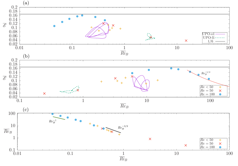
Figure 1: The variation of average mixing efficiency $\overline{\mathscr{E}}$ with: (a) average bulk Richardson number $\overline{Ri}_{B}$ and (b) average buoyancy Reynolds number $\overline{Re}_{B}$. The horizontal line is $\overline{\mathscr{E}}=1/6$, consistent with the upper bound of Osborn (1980). The closed loops mark the projections onto the time-dependent $(Ri_{B},\mathscr{E})$ and $(Re_{B},\mathscr{E})$ planes of the two unstable relative periodic orbits UPO-o1 (solid line) and UPO-l1 (dashed line) discussed in section 4. (c) shows the variation of $\overline{Re}_{B}$ with $\overline{Ri}_{B}$. Different symbols mark different values of $Re$. The red curve in (b) corresponds to $\overline{\mathscr{E}}=\overline{Re}_{B}^{-1/2}$, the large $Re_{B}$ behaviour suggested by Shih et al. (2005).

#	$Re$	$B$	$\overline{Ri}_{B}$	$\eta k_{\mathrm{max}}$	$\overline{\mathscr{E}}$	$\overline{Re}_{B}$	$l_{o}$	$Re_{\lambda}$
A1	20	1	0.325	2.7	0.0859	9.8	0.695	31.3
A2	30	1	0.235	2.0	0.1026	14.9	0.698	51.2
A3	30	5	0.525	1.8	0.0892	4.04	0.244	25.5
A4	40	5	0.489	1.5	0.114	4.64	0.226	52.1
A5	40	7.5	0.58	1.5	0.099	3.45	0.177	31.6
A6	40	10	0.835	1.6	0.096	1.94	0.124	23.6
B1	50	5	0.398	1.3	0.121	5.89	0.228	44.7
B2	50	10	0.608	1.3	0.112	3.21	0.141	44.1
B3	50	50	3.18	1.2	0.054	0.83	0.048	31.3
B4	50	100	14.95	1.4	0.038	0.25	0.022	45.9
C1	100	0.5	0.046	1.6	0.109	94.82	1.15	98.5
C2	100	0.75	0.065	1.6	0.129	65.19	0.86	92.5
C3	100	1.0	0.089	1.6	0.144	48.03	0.69	94.1
C4	100	1.5	0.126	1.6	0.156	31.41	0.50	91.2
C5	100	2.0	0.156	1.6	0.160	24.3	0.41	88.6
C6	100	5.0	0.278	1.5	0.153	10.8	0.22	76.2
C7	100	10.0	0.423	1.5	0.137	5.91	0.14	62.9

Table 1: Imposed parameters and diagnostic outputs for the three groups of simulations. The nondimensional Kolmogorov microscale is given by $\eta=Re^{-3/4}\overline{\mathcal{D}}^{-1/4}$ and is scaled by the maximum wavenumber allowable $k_{\mathrm{max}}=N/3$. Groups A and B have resolution $128\times 64^{2}$ and group C has $256\times 128^{2}$ to retain spectral convergence. The nondimensional Ozmidov length scale $l_{O}={\overline{\mathcal{D}}}^{1/2}/{B^{\frac{3}{4}}}$, the average buoyancy Reynolds number $\overline{Re}_{B}=\overline{\mathcal{D}}Re/B,$ the average bulk Richardson number $\overline{Ri}_{B}$ and the Taylor microscale Reynolds number $Re_{\lambda}=\mathcal{K}_{\mathrm{turb}}\sqrt{{10Re}/{\overline{\mathcal{D}}}}$ are also listed. Here we define $\mathcal{K}_{turb}=(1/2)\langle(\bm{u}-\overline{\bm{u}})^{2}\rangle_{V}$ and overbars are always time averages over the full $T=1000$ window.

4 Recurrent flow analysis

In order to determine what processes underpin the turbulence in our simulations, we use ‘recurrent flow analysis’. The general approach is as follows. First a simulation is conducted during which near recurrences are located in the chaotic trajectory. This is achieved by storing a historical record of state vectors and periodically checking the history against the current state vector. When an appropriately ‘near repeat’ is identified, it is stored for a later convergence attempt with a Newton-GMRES-hookstep algorithm. For more details on this approach see Chandler & Kerswell (2013); Lucas & Kerswell (2015). Here, we are interested in finding representative unstable periodic orbits (UPOs) with qualitatively different mixing properties in a broad range of flows, rather than identifying a large number of UPOs for a specific set of parameters. Therefore, we have identified five orbits in two broad classes: one class of two orbits found in the relatively weakly stratified simulation A1 with $Re=20$ and $B=1$, and the other class of three orbits in the more strongly stratified simulation B3 with $Re=50$ and $B=50$. The first class has $\overline{Re}_{B}\sim O(10)$, and we label it as class ‘o’, for ‘overturning’, while the second class has $\overline{Re}_{B}\sim O(1)$, and we label it as class ‘l’ for layered. We plot projections onto the time-dependent $(Ri_{B},\mathscr{E})$ and $(Re_{B},\mathscr{E})$ planes of the trajectories of characteristic relative periodic orbits UPO-o1 (solid line) and UPO-l1 (dashed line) on figures 1(a) and (b), demonstrating that these two classes do indeed have qualitatively different mixing properties, and also that these time-dependent properties are consistent with the time-averaged properties of the ‘full’ DNS.

No.	DNS	$Re$	$B$	$T_{p}$	$s_{x}$	$s_{z}$	$m_{y}$	$\Lambda^{-1}$	$N_{\lambda}$	$\overline{Re}_{B}$	$\max(\mathscr{E})$	$\overline{Ri}_{B}$	$\overline{\mathscr{E}}$
UPO-o1	A1	20	1	21.28	5.98	0.35	0	1.65	25	8.5	0.13	0.333	0.078
UPO-o2	A1	20	1	7.51	7.81	-0.06	0	2.30	27	8.9	0.097	0.265	0.067
UPO-l1	B3	50	50	8.75	0.016	0	0	0.211	7	0.62	0.07	3.17	0.052
UPO-l2	B3	50	50	8.74	0	0	0	0.207	6	0.63	0.058	3.13	0.048
UPO-l3	B3	50	50	9.21	0	0.007	0	0.116	6	0.57	0.051	4.64	0.045

Table 2: Table cataloguing the unstable recurrent flows showing the DNS from which they come (table 1), period $T_{p}$, relative shifts in $x$ and $z$ directions- $s_{x}$, $s_{z}$ discrete shift/reflect in $y$ $m_{y},$ inverse stability coefficient ($\Lambda^{-1}$, see Chandler & Kerswell (2013)), the number of unstable directions $N_{\lambda}$, $\overline{Re}_{B},$ maximum and time averaged mixing efficiency $\mathscr{E}$ and time averaged bulk Richardson number $\overline{Ri}_{B}$.

Table 2 lists properties of the converged orbits, including period, relative shifts due to the continuous symmetries in $x$ and $z,$ stability and some diagnostic averages. By comparison with the averages of the DNS in table 1, it is clear the UPOs are reproducing the bulk time-averages quite well. The projection of the trajectories onto the $(Re_{B},\mathcal{E})$ plane of the five converged orbits are plotted in figure 2, with greyscale colours representing the probability density function (p.d.f.) of the turbulent DNS. Notice that the darker colours represent regions where the turbulent trajectory spends more time, and lighter colours represent less frequent excursions to that part of phase space. For simulation B3, the ‘l’ class of converged UPOs sit across the darkest region of the p.d.f. where the turbulence spends most of its time but miss the higher efficiency, intermittent turbulent bursts that the DNS exhibits. Missing extreme events is a known failing of the recurrent flow analysis in some circumstances and is a topic of ongoing research, see Lucas & Kerswell (2015). However, for the ‘o’ class in simulation A1, the orbit UPO-o1 (in particular) appears to span the turbulent attractor well in this projection, missing only some very rare excursions to high $Re_{B}.$ As shown in table 2, the ‘o’ class orbits are considerably more unstable than the orbits in ‘l’ class.

In order to compare how the timescales of the UPOs relate to those exhibited by the turbulence, we plot in figure 3 the power spectra of the kinetic energy for the two DNS signals from which the UPOs have been extracted (i.e. A1 and B3). Vertical lines show that the the periods of the orbits are approximately coincident with observed frequencies. For simulation A1 the largest non-zero peak in the frequency spectrum occurs at approximately half the fundamental frequency observed in the UPOs, i.e. $f\approx 2\pi/15=0.42$ with the fundamental period around $7.5$, UPO-o1 having just under three such periods. For simulation B3 the periods of the orbits are on the edge of the main distribution of frequencies near $f=0.6.$ This is reasonable evidence that the timescales of the UPOs are representative of the typical timescales of the turbulence. We can also consider the buoyancy frequency and its influence on these cases. For simulation A1 where $B=1$, the background buoyancy frequency $N_{B}=\sqrt{(}B)=1$ so the timescale or ‘buoyancy period’ is $T_{N}=2\pi$ which is not far from the “fundamental period” we have established from the UPOs and spectrum. For B3, the buoyancy period $T_{N}=2\pi/\sqrt{(}50)\approx 0.9$ which is much faster than the timescales found in the spectrum. We find some signature of this frequency later in this section. Henceforth, we will focus attention on UPO-o1 and UPO-l1 since, having larger amplitude, they represent better proxies for the turbulence, although the dynamics within each class is broadly similar.

Figure 2: Projection onto the ($Re_{B},\mathscr{E}$) plane of the UPOs and the p.d.f. of the direct numerical simulations rendered in greyscale, with darker shades denoting that the turbulent trajectory spends more time there for: (a) class ‘o’ UPOs from simulation A1; and (b) class ‘l’ UPOs from simulation B3.

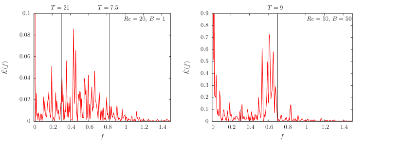
Figure 3: Power spectra for the kinetic energy $\hat{\mathcal{K}}(f)=\int_{T}\mathcal{K}(t)\mathrm{e}^{\mathrm{i}ft}{\rm d}t$ for the DNS signals from simulation A1 (left) and simulation B3 (right) with vertical lines showing approximately the periods of the UPOs extracted.

Figure 4: Time evolution of $Ri_{B}$ and $\mathscr{E}$ for: (a) UPO-o1; and (b) UPO-l1. Notice the correlation between $Ri_{B}$ and $\mathscr{E}$ for (a) and not for (b). The times highlighted in figures 5 and 6 are marked with stars.

Further evidence that the two classes are qualitatively different is shown in figure 4, where we plot the time dependence of $Ri_{B}$ and $\mathscr{E}$ for UPO-o1 and UPO-l1. The dynamics of UPO-o1 show relatively low $Ri_{B}$, strongly correlated to the mixing efficiency $\mathscr{E}$. There are three distinct sub-periods, each of which shows the bulk $Ri_{B}$ decrease to small values (indeed below the canonical value of $1/4$ for the linear instability of a stratified (vertical) shear layer given by the Miles-Howard theorem and frequently invoked as a diagnostic for overturning), followed by a maximum in mixing efficiency as the flow overturns. Such overturnings are visualised in figure 5, where snapshots of total density $\rho_{tot}$ and streamwise velocity $u$ are chosen before and after the final minimum of $Ri_{B}$ and near the subsequent maximum of $Ri_{B}$ following the peak $\mathscr{E}$ as marked on figure 4(a). (An animation of the time evolution of these fields is available as supplementary material.) The density field shows very distinct Kelvin-Helmholtz-like billows forming at $t=16.5$ where $\mathscr{E}$ and $Ri_{B}$ are beginning their growth phase, justifying the labelling of this UPO as being in class ‘o’. Of course, a bulk measure of the Richardson number does not capture the stability properties of the flow, and so in figure 5 we also plot the p.d.f. of $Ri_{G}(\bf{x})$ over the spatial domain at the same times, with a vertical line indicating $Ri_{G}=1/4$. These distributions show a striking increase of the proportion of the domain with $Ri_{G}<1/4$ prior to the overturning mixing event. This proportion then decreases with time, but does not vanish completely. Even in the periods of maximum bulk $Ri_{B}$ some regions of the domain remain with $Ri_{G}<1/4$. Apparently, it is necessary for an appreciable proportion of the domain to have a local gradient Richardson number $Ri_{G}<1/4$ before overturning is observed.

By contrast, as is apparent in figure 4(b), UPO-l1 has much larger overall $Ri_{B}$, seemingly uncorrelated to the behaviour of the markedly lower mixing efficiency $\mathscr{E}$. This is also apparent in the snapshots shown in figure 6 at the characteristic times marked on figure 4(b) (and the associated animations available as supplementary materials). No overturns occur, and the cycle of mixing behaviour is associated with straining or scouring motions drawing the perturbation density $\rho$ into thin layers, justifying the labelling as class ‘l’. The instantaneous p.d.f.s of the gradient $Ri_{G}$ plotted in figure 6 now show that nowhere in the domain has $Ri_{G}<1/4,$ even near $t=5.5$ when mixing efficiency is maximised. At peak $\mathscr{E},$ $t\approx 5.5,$ the snapshot of $\rho$ shows increased layers and arguably larger $\partial\rho/\partial z.$

In order to characterise the straining/scouring motions exhibited by the ‘l’ class, we examine the properites of the strain tensor

$$S_{ij}=\frac{1}{2}\left(\frac{\partial u_{i}}{\partial x_{j}}+\frac{\partial u_{j}}{\partial x_{i}}\right).$$

This tensor has three real eigenvalues, which we denote by $\tilde{\alpha},\,\tilde{\beta},\,\tilde{\gamma},$ referred to as the principal strains, which sum to zero in an incompressible flow. In general $\tilde{\alpha}>0$ and is therefore the stretching strain, $\tilde{\gamma}<0$ and is the compressional strain and the intermediate strain $\tilde{\beta}$ will control the three dimensionality, i.e. $\tilde{\beta}<0$ represent compression in two directions and fluid elements drawn into filaments, $\tilde{\beta}>0$ compression in one direction and fluid elements are drawn into sheets and $\tilde{\beta}=0$ a purely two-dimensional straining field. Figure 7 shows time series of the volume-averaged strains for the two characteristic UPOs, UPO-o1 and UPO-l1. In the overturning case, UPO-o1 shows that $\langle\tilde{\beta}\rangle_{V}$ is well correlated to the mixing efficiency, being positive and maximum when $\mathscr{E}$ is largest. This is in good agreement with Smyth (1999) who examined these strains for a freely decaying Kelvin-Helmholtz unstable shear layer; $\langle\tilde{\beta}\rangle_{V}$ is positive and has a distinct maximum during the second phase of the overturn where the flow becomes more isotropic (isotropic turbulence is observed to have the strains approximately in the ratio 3:1:-4 (Smyth, 1999; Ashurst et al., 1987)) and approaches zero in the quiescent periods as the flow relaxes back to the parallel shear mean flow. For the layered case, UPO-l1 is distinctly more anisotropic; the overall absolute values for $\langle\tilde{\beta}\rangle_{V}$ are an order of magnitude smaller and are actually negative for much of the cycle. At the point where the mixing efficiency is maximal ($t\approx 5.5$) $\langle\tilde{\beta}\rangle_{V}$ also has a maximum, but here this amounts to crossing the axes and $\langle\tilde{\alpha}\rangle_{V}\approx-\langle\tilde{\gamma}\rangle_{V}.$ Our interpretation is then that the flow approaches two-dimensionality where the mixing is largest and increased vertical gradients of $\rho$ are formed by the change in sign of $\langle\tilde{\beta}\rangle_{V}.$ This is in stark contrast to the overturning case where mixing has a more isotropic straining signature with large $\langle\tilde{\beta}\rangle_{V}.$ As a secondary observation, the higher frequency oscillations of $\langle\tilde{\beta}\rangle_{V}$ for UPO-l1 are of the order of $N=\sqrt{B}$ the buoyancy frequency, i.e. the buoyancy period here is $T_{N}=2\pi/\sqrt{50}\approx 0.9.$ This suggests that internal waves are also playing a role in this dynamical cycle.

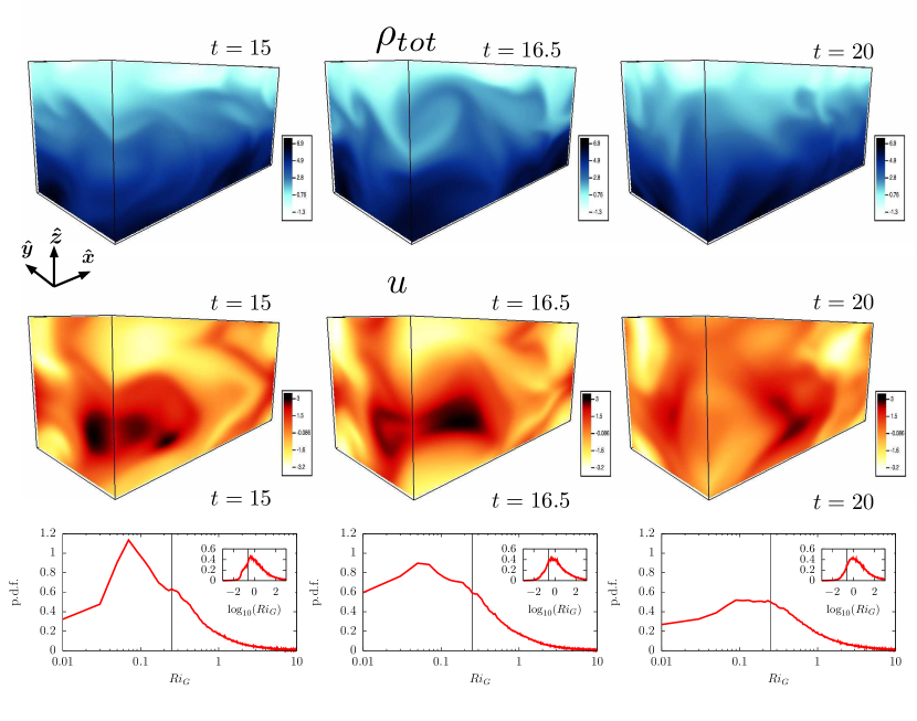
Figure 5: Three dimensional rendering of: (top) $\rho_{tot}=\rho-z$; (middle) $u$; and (bottom) p.d.f.s of $Ri_{G}$ in the entire computational domain at $t=15,\,16.5$ and $20$) (left to right) for UPO-o1. The p.d.f.s are computed with linear intervals of $Ri_{G},$ while the inset shows the result when distributing the intervals on a log scale. Vertical lines mark $Ri_{G}=1/4$.

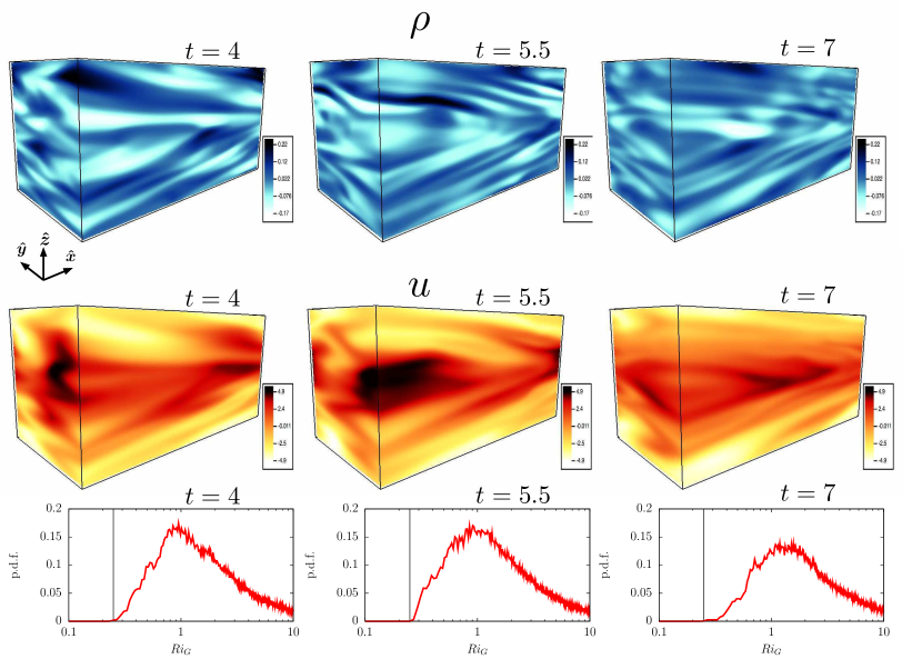
Figure 6: Three dimensional rendering of: (top) $\rho_{tot}=\rho-z$; (middle) $u$; and (bottom) p.d.f.s of $Ri_{G}$ in the entire computational domain at $t=4,\,5.5$ and $7$) (left to right) for UPO-l1. The p.d.f.s are computed with linear intervals of $Ri_{G},$ while the inset shows the result when distributing the intervals on a log scale. Vertical lines mark $Ri_{G}=1/4$.

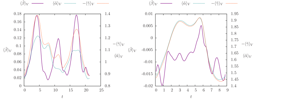
Figure 7: Time series of the volume averaged principal strains for UPO-o1 (left) and UPO-l1 (right). For the overturning case, peaks of $\mathscr{E}$ are coincident with large positive intermediate strain $\langle\tilde{\beta}\rangle_{V},$ nearer to the values of isotropic turbulence, where as the more layered case (right) is very anisotropic with small $\langle\tilde{\beta}\rangle_{V}$, approximately zero when $\mathscr{E}$ is largest.

5 Discussion and Conclusions

In this paper we have successfully applied recurrent flow analysis to stratified flows for the first time. As expected, success is restricted to relatively weak turbulence at modest Reynolds numbers. Nevertheless, the approach has still provided detailed insight into the sustaining mechanisms and mixing processes at work in these flows. In particular we have established that mixing can occur from two distinct mechanisms; overturning and scouring, consistently with the classification presented by Woods et al. (2010). Scouring is observed when stratification is strong and overturns when the stratification is weak enough to allow small gradient Richardson numbers. By examining the cycles in space and time we have demonstrated that the spatial distribution of local gradient $Ri_{G}$ is markedly skewed before high overturning mixing, but remains bounded from below by $1/4$ when scouring mixing dominates.

From this analysis it is clear that characterising mixing by appropriate measures of Richardson number is important from both a statistical and dynamical point of view, although we have also shown that weak mixing can be controlled by processes uncorrelated to $Ri_{G}$. Crucially, weaker average mixing may not be simply controlled by spatiotemporally intermittent shear instability, but by other scouring, straining processes, which may require other predictive diagnostics. Furthermore, since the bulk measures of Richardson number and buoyancy Reynolds number are functionally related, the results of our motivational DNS for horizontally forced, sustained turbulence suggest that an $(\overline{Ri}_{B},\overline{Re}_{B})$ parameterisation of mixing should be treated with caution, particularly since it proved difficult to access a strongly stratified, yet strongly turbulent regime, analogously to the situation arising in stratified plane Couette flow (Zhou et al., 2017).

One open question is the interplay between scouring and overturning. Clearly overturning shear instability will overwhelm any background straining or scouring motions, however it remains a challenge of rationalising spatiotemporal chaos to predict the switching between these processes. For instance simulation B3 shows that intermittent bursts can raise the local (in time) mixing efficiency, despite the majority of the mixing in this case being controlled by the straining and scouring layered motions characteristic of class ‘l’. Examination of a segment of the trajectory reaching large $\mathscr{E}$ in this case suggests straining and shear instability, saturating at various finite amplitudes, combine to populate the distribution of figure 1(b). Furthermore, as already widely discussed, research into exact coherent structures embedded in turbulent flows faces a serious challenge in the extension of methods to handle higher Reynolds numbers and spatially localised dynamics. It remains unclear whether such UPOs can be identified in ‘energetic’ stratified turbulence with $\overline{Re}_{B}\gtrsim O(100)$, yet it is of particular interest to understand whether the observed reduction of mixing efficiency at such high $\overline{Re}_{B}$ is associated with a qualitative change in mixing properties.

Acknowledgements. We extend our thanks, for many helpful and enlightening discussions, to Paul Linden, John Taylor, Stuart Dalziel and the rest of the ‘MUST’ team in Cambridge and Bristol. We also thank the three anonymous referees whose constructive comments have significantly improved the clarity of the manuscript. The source code used in this work is provided at https://bitbucket.org/dan_lucas/psgpu and the associated data including initialisation files and converged states can be found at www.repository.cam.ac.uk This work is supported by EPSRC Programme Grant EP/K034529/1 entitled ‘Mathematical Underpinnings of Stratified Turbulence’. The majority of the research presented here was conducted when DL was a postdoctoral researcher in DAMTP as part of the MUST programme grant.

References

- Ashurst et al. (1987) Ashurst, Wm. T., Kerstein, A. R., Kerr, R. M. & Gibson, C. H. 1987 Alignment of vorticity and scalar gradient with strain rate in simulated navier–stokes turbulence. Phys. Fluids 30 (8), 2343–2353.
- Chandler & Kerswell (2013) Chandler, G. J. & Kerswell, R. R. 2013 Invariant recurrent solutions embedded in a turbulent two-dimensional Kolmogorov flow. J. Fluid Mech. 722, 554–595.
- Cvitanović & Gibson (2010) Cvitanović, P. & Gibson, J. F. 2010 Geometry of the turbulence in wall-bounded shear flows: periodic orbits. Physica Scripta 142, 4007.
- Garaud et al. (2015) Garaud, Pascale, Gallet, Basile & Bischoff, Tobias 2015 The stability of stratified spatially periodic shear flows at low Péclet number. Physics of Fluids 27 (8), 084104–22.
- Ivey et al. (2008) Ivey, G. N., Winters, K. B. & Koseff, J. R. 2008 Density stratification, turbulence, but how much mixing? In Annu. Rev. Fluid Mech., , vol. 40, pp. 169–184.
- Kawahara & Kida (2001) Kawahara, G. & Kida, S. 2001 Periodic motion embedded in plane Couette turbulence: regeneration cycle and burst. J. Fluid Mech. 449, 291.
- Kawahara et al. (2012) Kawahara, G., Uhlmann, M. & van Veen, L. 2012 The significance of simple invariant solutions in turbulent flows. Annu. Rev. Fluid Mech. 44 (1), 203–225.
- Linden (1979) Linden, P. F. 1979 Mixing in stratified fluids. Geophys. Astrophys. Fluid Dyn. 13 (1), 3–23.
- Lucas et al. (2017) Lucas, D., Caulfield, C. P. & Kerswell, R. R. 2017 Layer formation in horizontally forced stratified turbulence: connecting exact coherent structures to linear instabilities , arXiv: 1701.05406v1.
- Lucas & Kerswell (2015) Lucas, D. & Kerswell, R. R. 2015 Recurrent flow analysis in spatiotemporally chaotic 2-dimensional Kolmogorov flow. Phys. Fluids 27 (4), 045106–27.
- Lucas & Kerswell (2017) Lucas, D. & Kerswell, R. R. 2017 Sustaining processes from recurrent flows in body-forced turbulence. Journal of Fluid Mechanics 817, R3–11.
- Maffioli et al. (2016) Maffioli, A., Brethouwer, G. & Lindborg, E. 2016 Mixing efficiency in stratified turbulence. J. Fluid Mech. 794, R3–12.
- Mashayek et al. (2017) Mashayek, A., Salehipour, H., Bouffard, D., Caulfield, C. P., Ferrari, R., Nikurashin, M., Peltier, W. R. & Smyth, W. D. 2017 Efficiency of turbulent mixing in the abyssal ocean circulation. Geophys. Res. Lett. 10.1002/2016GL072452.
- Mater & Venayagamoorthy (2014) Mater, B. D. & Venayagamoorthy, S. K. 2014 The quest for an unambiguous parameterization of mixing efficiency in stably stratified geophysical flows. Geophys. Res. Lett. 41 (13), 4646–4653.
- Osborn (1980) Osborn, T. R. 1980 Estimates of the Local Rate of Vertical Diffusion from Dissipation Measurements. Journal of Physical Oceanography 10 (1), 83–89.
- Peltier & Caulfield (2003) Peltier, W. R. & Caulfield, C. P. 2003 Mixing efficiency in stratified shear flows. Annu. Rev. Fluid Mech. 35, 135–167.
- Salehipour & Peltier (2015) Salehipour, H. & Peltier, W. R. 2015 Diapycnal diffusivity, turbulent Prandtl number and mixing efficiency in Boussinesq stratified turbulence. J. Fluid Mech. 775, 464–500.
- Salehipour et al. (2016) Salehipour, H., Peltier, W. R., Whalen, C. B. & MacKinnon, J. A. 2016 A new characterization of the turbulent diapycnal diffusivities of mass and momentum in the ocean. Geophys. Res. Lett. 43.
- Scotti & White (2016) Scotti, A. & White, B. 2016 The mixing efficiency of stratified turbulent boundary layers. J. Phys. Oceanogr. 46 (10), 3181–3191.
- Shih et al. (2005) Shih, L. H., Koseff, J. R., Ivey, G. N. & Ferziger, J. H. 2005 Parameterization of turbulent fluxes and scales using homogeneous sheared stably stratified turbulence simulations. J. Fluid Mech. 525, 193–214.
- Smyth (1999) Smyth, W. D. 1999 Dissipation-range geometry and scalar spectra in sheared stratified turbulence. J. Fluid Mech. 401, 209–242.
- van Veen et al. (2006) van Veen, L., Kida, S. & Kawahara, G. 2006 Periodic motion representing isotropic turbulence. Fluid Dyn. Res. 38 (1), 19–46.
- Woods et al. (2010) Woods, A. W., Caulfield, C. P., Landel, J. R. & A., Kuesters 2010 Non-invasive turbulent mixing across a density interface in a turbulent taylor-couette flow. J. Fluid Mech. 663, 347–357.
- Zhou et al. (2017) Zhou, Q., Taylor, J. R. & Caulfield, C. P. 2017 Self-similar mixing in stratified plane Couette flow for varying Prandtl number. J. Fluid Mech. 820, 86–120.