Effects of nonmagnetic disorder on the energy of Yu-Shiba-Rusinov states

Abstract

We study the sensitivity of Yu-Shiba-Rusinov states, bound states that form around magnetic scatterers in superconductors, to the presence of nonmagnetic disorder in both two and three dimensional systems. We formulate a scattering approach to this problem and reduce the effects of disorder to two contributions: disorder-induced normal reflection and a random phase of the amplitude for Andreev reflection. We find that both of these are small even for moderate amounts of disorder. In the dirty limit in which the disorder-induced mean free path is smaller than the superconducting coherence length, the variance of the energy of the Yu-Shiba-Rusinov state remains small in the ratio of the Fermi wavelength and the mean free path. This effect is more pronounced in three dimensions, where only impurities within a few Fermi wavelengths of the magnetic scatterer contribute. In two dimensions the energy variance is larger by a logarithmic factor because impurities contribute up to a distance of the order of the superconducting coherence length.

I Introduction

Adding magnetic impurities to an $s$-wave superconductor induces bound states, whose excitation energy falls within the superconducting gap. This prediction goes back to works of Yu, Shiba, and Rusinov (YSR) in the 1960s Yu (1965); Shiba (1968); Rusinov (1968). In the meantime, numerous aspects of YSR states have been considered theoretically Rusinov (1969); Zittartz et al. (1972); Hirschfeld et al. (1988); Balatsky et al. (2006); Morr and Y. (2006); Moca et al. (2008); Žitko et al. (2011); Yao et al. (2014); Hoffman et al. (2015); Kim et al. (2015); Meng et al. (2015); Žitko (2016) and YSR states are now routinely observed by scanning tunneling spectroscopy on superconductors Yazdani et al. (1997); Ji et al. (2008, 2010); Franke et al. (2011); Ménard et al. (2015); Ruby et al. (2015a); Hatter et al. (2015); Ruby et al. (2016); Choi et al. (2016); Kezilebieke et al. (2017); Heinrich et al. (2017).

Interest in YSR states was recently renewed for several reasons. One reason is that experimental progress admits measurements of subgap spectra with much higher resolution than previously possible. This has triggered experimental and theoretical work exploring the basic properties of YSR states in more detail. It was recently found that reducing the dimensionality of the superconducting host from three to two dimensions greatly increases the observed spatial extent of the YSR states, which is a consequence of the different power laws with which the YSR wavefunctions decay away from the impurity Ménard et al. (2015); Kezilebieke et al. (2017). Other recent work traced the origin of multiple YSR states to the crystal splitting of higher angular momentum channels Ruby et al. (2015a, 2016); Ji et al. (2008); Hatter et al. (2015); Choi et al. (2016).

Another reason is that chains of magnetic adatoms on superconductors have been proposed as a realization of a topological superconducting phase which harbors Majorana bound states at the ends of the chain, motivating several recent experimental studies of such systems Nadj-Perge et al. (2014); Ruby et al. (2015b); Pawlak et al. (2016); Feldman et al. (2017); Ruby et al. (2017). Majorana bound states are quasiparticles which are their own antiparticles and potential building blocks of a future topological quantum computer Kitaev (2003); Nayak et al. (2008). One way to think about this topological superconducting phase is in terms of an effective tight-binding model of hybridized YSR states Nadj-Perge et al. (2013); Pientka et al. (2013); Klinovaja et al. (2013); Braunecker and Simon (2013); Kim et al. (2014); Schecter et al. (2016).

It is an important question to which degree YSR bound states are sensitive to potential (nonmagnetic) impurities in the superconductor. In the context of individual magnetic impurities, strong sensitivity to potential impurities would make the YSR energies sample specific, reflecting the details of the impurity configuration in the vicinity of the magnetic atom. Similarly, topological superconductivity is known to be sensitive to disorder. Sensitivity of the YSR state to potential scatterers in the superconductor could thus be detrimental to the formation of a topological superconducting phase.

In this work, we characterize the sensitivity of YSR states in two and three dimensions to potential scatterers. We find that the YSR states are robust to disorder, even when the mean free path is shorter than the coherence length of the superconductor. The major condition for this robustness is that the disorder induced mean free path is large compared to the Fermi wavelength which is usually satisfied in conventional superconductors. Thus, our findings relax previous claims Hui et al. (2015) that ultraclean superconductors are required for disorder to introduce only a small perturbation. These earlier results do not include a discussion of the Fermi wavelength, which we find to be a crucial parameter when considering the robustness of the YSR energy. We refer to appendix A for a more detailed discussion of the origin of the discrepancy with Ref. Hui et al. (2015).

This paper is structured as follows. In Sec. II we introduce the model Hamiltonian on which our analysis is based. In Sec. III, we review the YSR wavefunctions in the absence of disorder and present a perturbative analysis of the effect of disorder on the YSR energies. Section IV introduces a scattering approach, which in an approximate analytical approach, allows us to reduce the effects of disorder on the YSR energy to two contributions which can be discussed qualitatively based on symmetry arguments and a random walk model. In addition, we also employ the scattering approach for a numerical calculation beyond perturbation theory and compare it to the results obtained by perturbation theory. Finally, we conclude in Sec. V.

II Model

The system we consider is described by the Bogoliubov-de Gennes Hamiltonian

$$H=\begin{pmatrix}H_{0}+V_{\uparrow}({\mathbf{r}})+U({\mathbf{r}})&\Delta\\ \Delta&-H_{0}-V_{\downarrow}({\mathbf{r}})-U({\mathbf{r}})\end{pmatrix},$$ (1)

where $H_{0}=p^{2}/2m-\hbar^{2}k_{\rm F}^{2}/2m$, with $m$ the (effective) mass and $k_{\rm F}$ the Fermi wavenumber, $\Delta$ the superconducting order parameter, which we choose to be real, $V_{\sigma}({\mathbf{r}})$ the impurity potential, and $U({\mathbf{r}})$ the disorder potential.

Following Refs. Yu, 1965; Shiba, 1968; Rusinov, 1968 we take the impurity to be a classical spin of magnitude $S$, located at the origin ${\mathbf{r}}=0$. Choosing the spin quantization axis along the impurity spin direction, the spin-dependent impurity potential has the form

$$V_{\sigma}({\mathbf{r}})=(V_{0}-JS\sigma)\delta_{\lambda}({\mathbf{r}}).$$ (2)

Here, $\delta_{\lambda}({\mathbf{r}})$ represents a short-ranged function with unit integral and range $\lambda\sim 1/k_{\rm F}$, $J$ is the exchange coupling strength, and $V_{0}$ is the strength of the potential scattering by the impurity.

For the disorder potential $U({\mathbf{r}})$, we take a Gaussian white noise model, for which $U({\mathbf{r}})$ has zero mean and variance

$$\left\langle U(\mathbf{r})U(\mathbf{r}^{\prime})\right\rangle=\frac{\hbar v_{\rm F}}{2\pi\nu_{0}\ell}\delta_{\lambda}\left(\mathbf{r}-\mathbf{r}^{\prime}\right),$$ (3)

where $\ell$ is the elastic mean free path, $v_{\rm F}=\hbar k_{\rm F}/m$ the Fermi velocity, and $\nu_{0}$ the density of states per spin direction. [In two dimensions ($d=2$) and three dimensions ($d=3$), one has $\nu_{0}=k_{\rm F}/2\pi\hbar v_{\rm F}$ and $\nu_{0}=k_{\rm F}^{2}/2\pi^{2}\hbar v_{\rm F}$, respectively.] For simplicity, we choose the same short-distance cutoff $\lambda$ for the disorder potential $U({\mathbf{r}})$ and for the impurity potential $V_{\sigma}({\mathbf{r}})$.

The characteristic length scales of the system are illustrated in Fig. 1. The superconductor is characterized by the clean-limit superconducting coherence length $\xi_{0}=\hbar v_{\rm F}/\Delta$. For weak-coupling superconductors, one has $k_{\rm F}\xi_{0}\gg 1$. Also, in superconductors that are good metals in the normal state, one has $k_{\rm F}\ell\gg 1$. We will assume that both inequalities are obeyed in the considerations that follow, but we will not make any assumptions concerning the relative magnitude of the mean free path $\ell$ and the coherence length $\xi_{0}$. Superconductors with $\ell\gg\xi_{0}$ are in the clean limit; superconductors with $\ell\ll\xi_{0}$ are in the dirty limit.

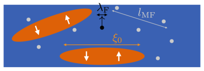
Figure 1: Sketch of the model used in this work and the relevant length scales. A magnetic impurity with a size comparable to the Fermi wavelength $\lambda_{F}$ is placed inside a superconductor. The coherence length $\xi_{0}$ corresponds to the size of Cooper pairs (orange) that form the superconducting ground state in the absence of disorder. Adding nonmagnetic disorder (gray circles) introduces a mean free path $\ell$.

III Perturbative approach

In the presence of the impurity potential $V$, the Bogoliubov-de Gennes equation

$$H\ket{\psi}=\varepsilon\ket{\psi},$$ (4)

with $H$ given by Eq. (1), has a bound-state solution with energy $|\varepsilon|<\Delta$. In this section, we review Rusinov’s original calculation of the bound-state energy $\varepsilon_{0}$ for a clean superconductor Rusinov (1968). We then use this as a starting point to calculate the shift $\delta\varepsilon=\varepsilon-\varepsilon_{0}$ to first order in the disorder potential $U$.

We start with the general radially symmetric solution of the Bogoliubov-de Gennes equation (4) for $r>\lambda$, where $\lambda$ is the range of the potential $V_{\sigma}({\mathbf{r}})$. For $k_{\rm F}\xi_{0}\gg 1$, this reads

$$\ket{\psi({\mathbf{r}})}=\frac{1}{\sqrt{\xi_{\varepsilon}}}\sum_{\pm}a_{\pm}\Phi_{\pm}(r)e^{-r/\xi_{\varepsilon}}\ket{\pm},$$ (5)

where $a_{\pm}$ are complex coefficients,

$$\xi_{\varepsilon}=\frac{\hbar v_{\rm F}}{\sqrt{\Delta^{2}-\varepsilon^{2}}}$$ (6)

is the energy-dependent coherence length, $\Phi_{\pm}(r)$ solves the radial Schrödinger equation at $\varepsilon=0$ in the absence of superconductivity and takes different forms in two and three dimensions,

$$\Phi_{\pm}(r)=\left\{\begin{array}[]{ll}\sqrt{\frac{k_{\rm F}}{4}}H_{0}^{\pm}(k_{\rm F}r)&d=2,\\ \sqrt{\frac{k_{\rm F}^{2}}{4\pi}}h_{0}^{\pm}(k_{\rm F}r)&d=3,\end{array}\right.$$ (7)

with $H^{\pm}$ and $h^{\pm}$ the Hankel and spherical Hankel functions, respectively, and $\ket{\pm}$ are two-component spinors,

$$\ket{\pm}=\frac{1}{\sqrt{2}}\begin{pmatrix}1\\ e^{\mp i\eta(\varepsilon)}\end{pmatrix},$$ (8)

with the Andreev phase

$$\eta(\varepsilon)=\arccos(\varepsilon/\Delta).$$ (9)

To determine the coefficients $a_{\pm}$ we use the boundary condition at $r=\lambda$ imposed by the magnetic impurity. Following Rusinov’s original derivation Rusinov (1968), we formulate this boundary condition in terms of scattering phase shifts $\phi_{\sigma}$ for electrons with spin $\sigma$. We may neglect the effect of superconductivity on the phase shifts $\phi_{\sigma}$ since $\lambda\ll\xi_{0}$. The scattering phases $\phi_{\sigma}$ can be related to the impurity potential (2) by Rusinov (1968); Clogston (1962); foo

$$\tan\phi_{\sigma}=-\pi\nu_{0}(V_{0}-\sigma JS).$$ (10)

We note that in the general solution (5) the upper component multiplied by $a_{+}$ ($a_{-}$) describes a radial wave for an electron with spin up moving away from (towards) the origin. Hence,

$$a_{+}=e^{2i\phi_{\uparrow}}a_{-}.$$ (11)

Similarly, the lower component multiplied by $a_{+}$ ($a_{-}$) describes a radial wave moving towards (away from) the origin for a hole in the spin-down band. Taking into account the phase factors $e^{\pm i\eta(\varepsilon)}$ in the lower component of the spinor (8), we find the relation

$$a_{-}e^{i\eta(\varepsilon)}=e^{-2i\phi_{\downarrow}}a_{+}e^{-i\eta(\varepsilon)}.$$ (12)

Combining these two equations we find the YSR-state energy

$$\varepsilon_{0}=\pm\Delta\cos(\phi_{\uparrow}-\phi_{\downarrow})$$ (13)

for a magnetic impurity in an (otherwise) clean superconductor. The solution (5) is properly normalized if $|a_{+}|=|a_{-}|=1$ (up to corrections that are small in the limit $k_{\rm F}\xi_{0}$, $\xi_{0}/\lambda\gg 1$). Note that $|\varepsilon_{0}|<\Delta$ if and only if $\phi_{\uparrow}\neq\phi_{\downarrow})$, i.e., if the impurity is magnetic.

We now calculate the change $\delta\varepsilon$ of the energy of the YSR state to first order in the disorder potential $U({\mathbf{r}})$. We assume that $U({\mathbf{r}})=0$ for $r<\lambda$, i.e., the disorder potential does not overlap with the potential of the magnetic impurity. To first order in $U({\mathbf{r}})$ the change $\delta\varepsilon$ is

$$\delta\varepsilon=\int\mathrm{d}\mathbf{r}\bra{\psi({\mathbf{r}})}U(\mathbf{r})\tau_{z}\ket{\psi({\mathbf{r}})},$$ (14)

where $\tau_{z}$ is the Pauli matrix in particle-hole space and the spinor wavefunction $\ket{\psi({\mathbf{r}})}$ is given by the general solution (5), with the coefficients $a_{\pm}$ satisfying the relations (11) and (12). Using the relation $\Phi_{+}(k_{\rm F}r)=[\Phi_{-}(k_{\rm F}r)]^{*}$ this can be simplified as

$$\delta\varepsilon= \sin\eta(\varepsilon_{0})\int\mathrm{d}{\mathbf{r}}U({\mathbf{r}})e^{-2r/\xi_{\varepsilon_{0}}}$$

$$\,\mbox{}\times\mathrm{Im}\,e^{-i\eta(\varepsilon_{0})+2i\phi_{\uparrow}}[\Phi_{+}(r)]^{2}.$$ (15)

Using the correlator (3), we obtain the variance

$$\langle\delta\varepsilon^{2}\rangle= \,\frac{2\hbar v_{\rm F}}{\pi\nu_{0}\ell\xi_{\epsilon_{0}}^{2}}\sin^{2}\eta(\varepsilon_{0})$$ (16)

$$\,\mbox{}\times\int d{\mathbf{r}}\left\{\mathrm{Im}\,e^{-i\eta(\varepsilon_{0})+2i\phi_{\uparrow}}[\Phi_{+}(r)]^{2}\right\}^{2}e^{-4r/\xi_{\varepsilon_{0}}}.$$

In two dimensions the main contribution to the integral (16) comes from $r\sim\xi_{\varepsilon_{0}}$. The integral is convergent at the lower limit $r\downarrow 0$, so that the short-distance cutoff $\lambda$ can be taken to zero. We then find

$$\langle\delta\varepsilon^{2}\rangle=\frac{\Delta^{2}(\xi_{0}/\xi_{\varepsilon_{0}})^{4}}{\pi k_{\rm F}\ell}\log(k_{\rm F}\xi_{\varepsilon_{0}}).$$ (17)

In three dimensions the integral (16) is dominated by short distances $r\sim\lambda\sim k_{\rm F}^{-1}$ and the short-distance cutoff $\lambda$ is needed to ensure convergence. In this case we find

$$\langle\delta\varepsilon^{2}\rangle\sim\frac{\Delta^{2}(\xi_{0}/\xi_{\varepsilon_{0}})^{4}}{k_{\rm F}\ell},$$ (18)

where a numerical prefactor depends on the precise way in which the short-distance regularization is implemented. Note that in three dimensions and with $\varepsilon_{0}$ well inside the gap such that $\xi_{0}/\xi_{\varepsilon_{0}}\sim 1$, the variance $\langle\delta\varepsilon^{2}\rangle$ does not depend on $k_{\rm F}\xi_{\varepsilon_{0}}$.

In two dimensions the root-mean-square fluctuations are parametrically smaller than the superconducting gap $\Delta$ if the condition $k_{\rm F}\ell\gg\log(k_{\rm F}\xi_{0})$ is met. This condition only weakly depends on the superconducting coherence length $\xi_{0}$. In three dimensions the condition is $k_{\rm F}\ell\gg 1$, which is independent of $\xi_{0}$. The latter condition $k_{\rm F}\ell\gg 1$ is typically met in superconductors that are good metals in the normal state, such as Pb or Al.

IV Scattering approach

In this section, we present a numerical calculation of the YSR-state energies that takes higher-order contributions in the disorder potential $U({\mathbf{r}})$ into account. The calculation makes use of a relation between the YSR-state energy $\varepsilon$ and the scattering matrix $S(\varepsilon)$ of the superconductor for radial waves moving towards and from the origin ${\mathbf{r}}=0$. We first describe this relation and the calculation of $S(\varepsilon)$ separately, and then proceed with a calculation of the variance $\langle\delta\varepsilon^{2}\rangle$.

IV.1 Relation between YSR-state energy and scattering amplitudes

To define the scattering matrix $S$ we introduce a narrow shell $r_{0}<r<r_{0}+\delta r$ around the impurity in which the superconducting order parameter $\Delta$ as well as the potentials $V$ and $U$ are set to zero. (At the end of the calculation, we will send the shell width $\delta r\to 0$.) We choose $r_{0}\sim\lambda\lesssim 1/k_{\rm F}$. The solution of the Bogoliubov-de Gennes equation may be assumed to be radially symmetric, so that it can be expanded as

$$\ket{\psi({\mathbf{r}})}=\sum_{\pm}\left[a_{{\rm e},\pm}\ket{\Phi_{{\rm e},\pm}({\mathbf{r}})}+a_{{\rm h},\pm}\ket{\Phi_{{\rm h},\pm}({\mathbf{r}})}\right],$$ (19)

where $\ket{\Phi_{{\rm e},\pm}}$ and $\ket{\Phi_{{\rm e},\pm}}$ represent flux-normalized electron-like (e) and hole-like (h) waves propagating radially outward ($+$) or inward ($-$). In two dimensions one has

$$\ket{\Phi_{{\rm e},\pm}({\mathbf{r}})} =\sqrt{\frac{k_{\rm F}}{4v_{{\rm F}}}}H_{0}^{\pm}(k_{\rm F}r)\begin{pmatrix}1\\ 0\end{pmatrix},$$

$$\ket{\Phi_{{\rm h},\pm}({\mathbf{r}})} =\sqrt{\frac{k_{\rm F}}{4v_{{\rm F}}}}H_{0}^{\mp}(k_{\rm F}r)\begin{pmatrix}0\\ 1\end{pmatrix},$$ (20)

whereas in three dimensions

$$\ket{\Phi_{{\rm e},\pm}({\mathbf{r}})} =\sqrt{\frac{k_{\rm F}^{2}}{4\pi v_{{\rm F}}}}h_{0}^{\pm}(k_{\rm F}r)\begin{pmatrix}1\\ 0\end{pmatrix},$$

$$\ket{\Phi_{{\rm h},\pm}({\mathbf{r}})} =\sqrt{\frac{k_{\rm F}^{2}}{4\pi v_{{\rm F}}}}h_{0}^{\mp}(k_{\rm F}r)\begin{pmatrix}0\\ 1\end{pmatrix}.$$ (21)

The solution of the Bogoliubov-de Gennes equation for $r>r_{0}+\delta r$ yields two linear relations for the four amplitudes $a_{{\rm e},\pm}$ and $a_{{\rm h},\pm}$, which have the general form

$$\begin{pmatrix}a_{{\rm e},-}\\ a_{{\rm h},-}\end{pmatrix}=S(\varepsilon)\begin{pmatrix}a_{{\rm e},+}\\ a_{{\rm h},+}\end{pmatrix},\ \ S=\begin{pmatrix}r_{\text{ee}}&r_{\text{eh}}\\ r_{\text{he}}&r_{\text{hh}}\end{pmatrix}.$$ (22)

The matrix $S$ is the scattering matrix of the superconductor for radial waves around the origin ${\mathbf{r}}=0$. The coefficients $r_{\rm ee}$ and $r_{\rm hh}$ are the amplitudes for normal reflection of electrons and holes, respectively, whereas $r_{\rm he}$ and $r_{\rm eh}$ describe Andreev reflection of electrons into holes and vice versa. Time-reversal symmetry and particle-hole symmetry enforce the constraints

$$S(\varepsilon)=S^{\rm T}(\varepsilon)=\tau_{y}S(-\varepsilon)^{*}\tau_{y},$$ (23)

where $\tau_{y}$ is a Pauli matrix in particle-hole space.

In the absence of the disorder potential $U({\mathbf{r}})$, one has $r_{\rm ee}=r_{\rm hh}=0$, and $r_{\rm eh}=r_{\rm he}=e^{-i\eta(\varepsilon)}$, with $\eta(\varepsilon)$ defined in Eq. (9). This reproduces Eq. (5). In the presence of the disorder potential $U({\mathbf{r}})$, all four coefficients are in general nonzero. As we will show below, the difference with the clean case is small when $k_{\rm F}\ell\gg 1$, so that we may write

$$S(\varepsilon)=e^{-i\eta(\varepsilon)}\tau_{x}\left(\openone-i\delta A(\varepsilon)\right),$$ (24)

where $\delta A(\varepsilon)$ is small. The conditions that $S(\varepsilon)$ be unitary, symmetric, and particle-hole symmetric imply

$$\delta A(\varepsilon)=\delta A(\varepsilon)^{\dagger}=\tau_{x}\delta A(\varepsilon)^{\rm T}\tau_{x}=-\tau_{z}\delta A(-\varepsilon)\tau_{z}.$$ (25)

We therefore parameterize

$$\delta A(\varepsilon)=\begin{pmatrix}\delta\eta(\varepsilon)&\delta r(\varepsilon)\\ \delta r(\varepsilon)^{*}&\delta\eta(\varepsilon)\end{pmatrix},$$ (26)

where $\delta r(\varepsilon)$ is a complex, symmetric function of energy $\varepsilon$, which represents disorder-induced normal reflection, whereas $\delta\eta(\varepsilon)$ is a real, antisymmetric function of $\varepsilon$, which represents a disorder-induced shift of the Andreev reflection phase $\eta(\varepsilon)$.

As discussed above, the solution of the Bogoliubov-de Gennes equation for $r<r_{0}$ yields two additional relations between the amplitudes $a_{{\rm e},\pm}$ and $a_{{\rm h},\pm}$,

$$a_{{\rm e},+}=e^{2i\phi_{\uparrow}}a_{{\rm e},-},\ \ a_{{\rm h},-}=e^{-2i\phi_{\downarrow}}a_{{\rm h},+}.$$ (27)

Note that in Eq. (27), we assumed that the size of the magnetic impurity is small compared to the coherence length, corresponding to $k_{\rm F}\xi_{0}\gg 1$. By taking this limit we can neglect scattering from electrons to holes at the position of the impurity.

A nontrivial solution of Eqs. (22) and (27) exists if

$$\det\left[\begin{pmatrix}e^{2i\phi_{\uparrow}}&0\\ 0&e^{-2i\phi_{\downarrow}}\end{pmatrix}S(\varepsilon)-\begin{pmatrix}1&0\\ 0&1\end{pmatrix}\right]=0.$$ (28)

This gives

$$\varepsilon= \varepsilon_{0}+\delta\varepsilon,$$

$$\delta\varepsilon= \frac{\xi_{0}\Delta}{\xi_{\varepsilon_{0}}}\left[\delta\eta(\varepsilon_{0})+\mbox{Re}\,e^{-i(\phi_{\uparrow}+\phi_{\downarrow})}\delta r(\varepsilon_{0})\right],$$ (29)

to lowest order in $\delta A$. This equation is central to our analysis, since it allows us to calculate the energy shift $\delta\varepsilon$ from the scattering matrix $S$.

IV.2 Qualitative discussion

Next, we employ a semiclassical picture to qualitatively discuss why both $\delta\eta$ and $\delta r$ are expected to be small. Within this semiclassical picture, Andreev reflection is retroreflection, i.e., after Andreev reflection a hole retraces the path of the incident electron (or vice versa). Because the phases of electron and hole wavefunctions are correlated, see, e.g., Eq. (5), no net phase is accumulated, with the exception of the Andreev phase $\eta(\varepsilon)$. If $k_{\rm F}\ell\gg 1$ this semiclassical picture remains valid in the presence of a disorder potential $U({\mathbf{r}})$. This explains why $\delta\eta$, corresponding to a shift of the Andreev phase, is small if $k_{\rm F}\ell\gg 1$.

In fact, since $\delta\eta(\varepsilon)$ is an antisymmetric function of $\varepsilon$, one must have $\delta\eta(0)=0$, so that there is no contribution to the YSR-state energy shift from the phase shift $\delta\eta$ for YSR states with energy near the center of the superconducting gap. Instead, for small YSR-state energies, the residual disorder-induced fluctuations are dominated by the normal reflection amplitude $\delta r$. An estimate of the size of the YSR-energy fluctuations can be obtained by estimating $\delta r$ as the amplitude that a particle returns to the origin ${\mathbf{r}}=0$ (up to a distance $1/k_{\rm F}$) within a time $\xi_{\varepsilon}/v_{\rm F}$. In the two-dimensional case we then find for the dirty superconductor limit $\xi_{0}\gg\ell$

$$|\delta r(\varepsilon)|^{2}\sim \,\int_{\lambda/v_{\rm F}}^{\ell/v_{\rm F}}dt\frac{1}{k_{\rm F}\ell t}+\int_{\ell/v_{\rm F}}^{\xi_{\varepsilon}/v_{\rm F}}dt\frac{2}{k_{\rm F}\ell t}$$

$$\sim \,\frac{1}{k_{\rm F}\ell}\log(k_{\rm F}\xi_{\varepsilon}^{2}/\ell).$$ (30)

The first integral covers ballistic propagation times $t\lesssim\tau$ and the second diffusive times $t\gtrsim\tau$, where $\tau=\ell/v_{\rm F}$ is the elastic mean free time. The integrands give the return probabilities per unit time, which, in the diffusive regime, is multiplied by a factor two due to coherent backscattering. In the second line the short-distance cutoff $\lambda$ was replaced by $1/k_{\rm F}$. In the ultraclean limit $\xi_{0}\ll\ell$ the second term in Eq. (30) is absent and the upper integration limit in the first is $\xi_{\varepsilon}$, which gives

$$|\delta r(\varepsilon)|^{2}\sim\frac{1}{k_{\rm F}\ell}\log(k_{\rm F}\xi_{\varepsilon})$$ (31)

In three dimensions, the return probability is dominated by the ballistic regime $t\lesssim\tau$ and one finds

$$|\delta r(\varepsilon)|^{2}\sim\int_{\lambda/v_{\rm F}}^{\tau}dt\frac{1}{k_{\rm F}^{2}\ell v_{\rm F}t^{2}}\sim\frac{1}{k_{\rm F}\ell}.$$ (32)

In three dimensions, the estimate is consistent with the smallness of the first-order perturbation theory results of Sec. III. In two dimensions and in the dirty limit, multiple scattering changes the argument of the logarithm in Eq. (30) by a factor $\xi_{\epsilon}/\ell$ compared to the perturbative result (17).

IV.3 Numerical calculation of the scattering matrix

Our strategy for an efficient numerical calculation can be outlined as follows. First, we slice the superconductor into thin circular ($d=2$) or spherical ($d=3$) pieces, as illustrated in Fig. (2), and calculate the scattering matrix for each piece. Next, we add the pieces together by concatenating their scattering matrices to obtain the total scattering matrix $S(\varepsilon)$. Finally, using Eqs. (24) and (29) we can relate this scattering matrix to the energy of the YSR state.

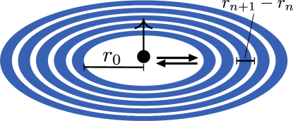
Figure 2: Sketch of the numerical method in two dimensions. The disordered superconductor is cut into thin circular slices (blue), with infinitesimally thin clean, metallic shells (white) in between. The scattering matrices of the slices are calculated in the narrow limit and combined into the full scattering matrix $S(\varepsilon)$, which describes the reflection of spherical symmetric waves (black) that are propagating from the magnetic impurity into the bulk.

Note that within this approach, we need to include non-zero angular momentum channels due to two reasons. First, disorder breaks rotational symmetry thus mixing different angular momentum modes. Second, the modes defined in Eq. (21) describe all propagation modes at radii $k_{\rm{F}}r\lesssim 1$. There, non-zero angular momentum modes are evanescent. This can be seen by considering the spherical representation of the momentum operator, which results in a repulsive potential that diverges $\sim 1/r^{2}$ at the origin for all modes but the zero angular momentum one. However, when going to larger radii non-zero angular momentum modes start to propagate and thus cannot be excluded.

Our approach starts, by formally inserting a sequence of $N+1$ infinitesimally thin ideal shells into the disordered superconductor at radii $r_{n}$, $n=0,1,\ldots,N$. Within these shells the superconducting order parameter $\Delta$ and the impurity potential $U({\mathbf{r}})$ are zero. The distance between the shells is $r_{n+1}-r_{n}\ll\ell$. In each shell the wavefunction can be expanded as [compare with Eq. (19)]

$$\ket{\psi({\mathbf{r}})}=\sum_{\nu}a^{(n)}_{\nu}\ket{\Phi_{\nu}({\mathbf{r}})},$$ (33)

where $\nu$ is a composite index representing particle/hole degrees of freedom (e or h), propagation direction (radially outward, $+$, or inward, $-$, and the angular momentum label $m$ (in two dimensions) or the angular momentum labels $l$, $m$ (in three dimensions).

The flux-normalized basis functions $\ket{\Phi_{\nu}}$ are

$$\ket{\Phi_{{\rm e},m\pm}({\mathbf{r}})} =\sqrt{\frac{k_{\rm F}}{4v_{{\rm F}}}}H_{m}^{\pm}(k_{\rm F}r)e^{im\varphi}\begin{pmatrix}1\\ 0\end{pmatrix},$$

$$\ket{\Phi_{{\rm h},m\pm}({\mathbf{r}})} =\sqrt{\frac{k_{\rm F}}{4v_{{\rm F}}}}H_{m}^{\mp}(k_{\rm F}r)e^{im\varphi}\begin{pmatrix}0\\ 1\end{pmatrix}$$ (34)

in two dimensions and

$$\ket{\Phi_{{\rm e},lm\pm}({\mathbf{r}})} =\sqrt{\frac{k_{\rm F}^{2}}{4\pi v_{{\rm F}}}}h_{l}^{\pm}(k_{\rm F}r)Y_{lm}(\theta,\varphi)\begin{pmatrix}1\\ 0\end{pmatrix},$$

$$\ket{\Phi_{{\rm h},lm\pm}({\mathbf{r}})} =\sqrt{\frac{k_{\rm F}^{2}}{4\pi v_{{\rm F}}}}h_{l}^{\mp}(k_{\rm F}r)Y_{lm}(\theta,\varphi)\begin{pmatrix}0\\ 1\end{pmatrix}$$ (35)

in three dimensions, where the $Y_{lm}(\theta,\phi)$ are spherical harmonics and the $H_{m}$ ($h^{\pm}_{l}$) are (spherical) Hankel functions. The solution of the Bogoliubov-de Gennes equation for $r_{n}<r<r_{n+1}$ gives a linear relationship between the coefficients $a^{(n)}$ and $a^{(n+1)}$, which has the form (vector notation is implied for all indices not listed explicitly)

$$\begin{pmatrix}a^{(n)}_{-}\\ a^{(n+1)}_{+}\end{pmatrix}={\cal S}^{(n)}(\varepsilon)\begin{pmatrix}a^{(n+1)}_{-}\\ a^{(n)}_{+}\end{pmatrix}$$ (36)

where ${\cal S}^{(n)}(\varepsilon)$ is the scattering matrix between the shells at $r_{n}$ and $r_{n+1}$.

If $r_{n+1}-r_{n}$ is much smaller than the mean free path $\ell$, the scattering matrix ${\cal S}^{(n)}(\varepsilon)$ can be calculated using the Born approximation,

$${\cal S}^{(n)}=[\openone-i{\cal T}^{(n)}/2][\openone+i{\cal T}^{(n)}/2]^{-1},$$ (37)

with

$${\cal T}^{(n)}_{\nu^{\prime}\nu}=\int_{r_{n}<r<r_{n+1}}d{\mathbf{r}}\bra{\psi_{\nu^{\prime}}({\mathbf{r}})}H^{\prime}_{\varepsilon}\ket{\psi_{\nu}({\mathbf{r}})},$$ (38)

with $H^{\prime}_{\varepsilon}=\Delta\tau_{x}+U({\mathbf{r}})\tau_{z}-\varepsilon$. We refer to the appendix for explicit expressions for the matrices ${\cal T}^{(n)}$.

To truncate the hierarchy of Eqs. (36) we set the disorder potential $U({\mathbf{r}})$ to zero for $r>r_{N}$, which gives the relation

$$a^{(N)}_{-}=e^{-i\eta(\varepsilon)}\tau_{x}a^{(N)}_{+}.$$ (39)

Further, for nonzero angular momentum indices $m$ or $l$ the Hankel functions $H_{m}$ and $h_{l}$ diverge for $k_{\rm F}r\lesssim\pi|m|/2$, $k_{\rm F}r\lesssim\pi l/2$, respectively. In that case regularity of $\ket{\psi({\mathbf{r}})}$ imposes that the corresponding coefficients $a_{+}^{(n)}$ and $a_{-}^{(n)}$ must be equal. In particular, we have

$$a_{{\rm e},+(l)m}^{(0)}=a_{{\rm e},-(l)m}^{(0)},\ \ a_{{\rm h},+(l)m}^{(0)}=a_{{\rm h},-(l)m}^{(0)}$$ (40)

for all $m\neq 0$ ($d=2$) or $l>0$ ($d=3$). Similarly, this observation allows us to truncate the sum over modes $l$ and $m$ to the number of propagating angular momentum modes at the largest distance required for the calculation of $S(\varepsilon)$, which is $r\sim\xi_{\varepsilon}$.

Combining Eqs. (36), (39), and (40) we can eliminate all amplitudes $a^{(n)}$ with $n\geq 1$ and calculate the scattering matrix $S(\varepsilon)$ describing the (Andreev) reflection of radially outgoing waves at the origin. The procedure becomes numerically exact in the limit $r_{n+1}-r_{n}\to 0$, $r_{N}\to\infty$. In practice, to achieve convergence it is sufficient that $r_{n+1}-r_{n}\lesssim\ell$ and if $r_{N}\sim\xi_{\varepsilon}$ because of the exponential decay of the wavefunction in the superconductor. In the numerical simulations, the short-distance cutoff is fixed to $r_{0}=0$ in two and $r_{0}=1/k_{\rm F}$ in three dimensions.

Figure 3 shows examples of the convergence behaviors in two and three dimensions. In two dimensions the numerical scattering matrix calculation converges slowly, in agreement with results from perturbation theory which predicts a logarithmic convergence at a length scale of the order of the coherence length. In contrast, our numerical results for three dimensional systems converge after a few Fermi wavelengths $2\pi/k_{\rm F}$ and also agree well with our results derived by perturbation theory.

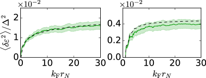
Figure 3: YSR energy shift (solid lines) versus disorder cutoff length $r_{N}$ in two dimensions (left panel) and three dimensions (right panel), obtained from the numerical scattering approach. We choose $\xi/\ell=10$ with $k_{\rm F}\ell=100$. When including the cutoff $r_{N}$, our perturbative approach (dashed lines) fits well with the numerical results. The shaded region shows the numerical standard error.

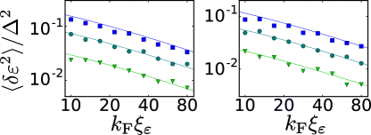
Figure 4: YSR energy variance versus $k_{\rm F}\xi_{\varepsilon}$ in two dimensions. The data points are for $\xi_{\varepsilon}/\ell=0.5$ (triangles), $1$ (circles) and $2$ (squares). The scattering phase shifts $\phi_{\uparrow}=-\phi_{\downarrow}$ are chosen such that YSR energy in the absence of disorder is $\varepsilon/\Delta=0$ (left) and $\varepsilon/\Delta=0.37$ (right). The solid lines show the lowest-order perturbation theory result from Eq. (17). Error bars are of the size of the markers.

In Fig. 4 we show the variance of the YSR energy for two dimensions. The numerical results confirm that the fluctuations become small in the limit of large $k_{\rm F}\ell$, while keeping $\ell/\xi_{\varepsilon}$ constant, quantitatively consistent with the result of lowest-order perturbation theory in the disorder potential $U({\mathbf{r}})$. Logarithmic corrections to the perturbative results are expected to occur deep in the dirty limit, see Eq. (30).

For comparison with the numerical results in three dimensions, we have repeated the perturbative calculation of Sec. III with the disorder potential set to zero for $r<r_{0}=1/k_{\rm F}$. In this case we find

$$\langle\delta\varepsilon^{2}\rangle=\frac{\Delta^{2}(\xi_{0}/\xi_{\varepsilon_{0}})^{4}}{k_{\rm F}\ell}$$ (41)

$$\times\left(c_{0}+\frac{c_{1}-2\log(k_{\rm F}\xi_{\varepsilon})}{k_{\rm F}\xi_{\varepsilon}}-\frac{c_{3}+c_{4}\cos\eta}{k_{\rm F}^{2}\xi_{\varepsilon}^{2}}+\cdots\right)$$

to second order in $1/k_{\rm F}\xi_{\varepsilon}$. The coefficients read $c_{0}\approx 0.45$, $c_{1}\approx 2.59$, $c_{3}\approx 5.87$ and $c_{4}\approx 2.71$. To leading order this simplifies to the asymptotic form in Eq. (18). The agreement of the higher order result (41) with the numerics is excellent for all values of $k_{\rm F}\xi_{\varepsilon}$ considered; the leading order agrees for large values of $k_{\rm F}\xi_{\varepsilon}$ only, see Fig. 5. Additional data for parameters deeper in the dirty limit and at fixed $k_{\rm F}$ and $\xi_{0}$ are provided in appendix B.

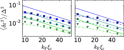
Figure 5: YSR energy variance in three dimensions, as a function of $k_{\rm F}\xi_{\varepsilon}$ at fixed ratios $\xi_{\varepsilon}/\ell$. The parameters are the same as in Fig. 4. The dashed and solid curves give the perturbative result (41) and its leading term, respectively.

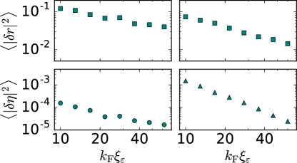
Figure 6: Comparison of the two contributions $\delta r$ and $\delta\eta$ to the superconductor scattering matrix $S(\varepsilon)$, in two (left) and three (right) dimensions. See Eq. (26). We choose a ratio $\xi_{0}/\ell=1$ and energy $\varepsilon/\Delta=0.15$. The contribution from normal reflection dominates in two as well as in three dimensions.

Our approach also allows us to separate contributions to the YSR energy variance arising from fluctuations of the Andreev phase and normal reflection, see Eq. (29). The two contributions to $\langle\delta\varepsilon^{2}\rangle$ are shown in Fig. 6 for $\varepsilon/\Delta=0.15$. The figure shows that the main contribution to $\langle\delta\varepsilon^{2}\rangle$ comes from normal reflection. This is consistent with the fact that fluctuations of the Andreev phase $\eta(\varepsilon)$ have an additional smallness because $\delta\eta(\varepsilon)$ is an antisymmetric function of energy.

V Conclusion

In this work we have analyzed the variance of the YSR energy due to nonmagnetic disorder in both two and three dimensions. Mapping this problem to a scattering ansatz for electrons and holes close to the magnetic impurity allowed us to reduce the effects of nonmagnetic disorder to two separate contributions.

First, the Andreev phase, which is picked up when an electron is Andreev reflected as a hole or vise versa, starts fluctuating as a function of disorder configuration. Using time reversal and particle hole symmetry, we have argued that this contribution is expected to be negligible in the limit $k_{\text{F}}\ell,\,k_{F}\xi_{\varepsilon}\gg 1$. Numerical calculations confirmed this prediction.

Second, disorder can flip the momentum and lead to a finite normal reflection amplitude for electrons or holes propagating from the impurity into the superconductor. We find that the normal reflection probability is small if $k_{\rm F}\ell\gg\log\left[k_{\rm F}\xi_{\varepsilon}\max(1,\xi_{\epsilon}/\ell)\right]$ and $k_{\rm F}\ell\gg 1$ in two and three dimensions, respectively. Importantly YSR states can be robust to disorder even in the limit of a dirty superconductor.

Finally, we found that in three dimensions only disorder within a few Fermi wavelengths of the magnetic impurity contributes to the YSR energy variance. This is in contrast to two dimensions, where disorder from distances up to the coherence length contributes.

Our results relax earlier claims Hui et al. (2015), which suggested that at $\ell$ of the order of $\xi_{0}$ the width of YSR energy distribution becomes of the order of the superconducting gap. Our findings show that $\lambda_{\rm F}$ is a crucial parameter to be included into the discussion and that this typically leads to a negligible influence of disorder.

Our findings also have implications for one dimensional topological superconductors, that are formed by dilute classical adatom chains. These systems can be described by effective tight-binding models Pientka et al. (2015). (Note, however, that current experiments may well be in a rather different limit in which the hybridization of the adatom d levels plays an important role Nadj-Perge et al. (2014); Ruby et al. (2015b); Feldman et al. (2017); Pawlak et al. (2016); Ruby et al. (2017).) The on-site energies in these models are immune to disorder, if the conditions are met that we derived in this work for the single Shiba states. This leaves the discussion of the tunneling and pairing strengths. If the distance $d$ between the impurities is small compared to $\ell$, we expect the influence of disorder on the nearest neighbor hopping and pairing terms to be suppressed by a factor $d/\ell\sim 1/k_{\rm F}\ell$. However, previous studies have shown Pientka et al. (2013, 2014), that in a clean system with $k_{\rm F}\xi_{0}\gg k_{\rm F}d\gg 1$, tunneling is following a long-range, $1/r$ power law. Thus, strictly speaking, more than nearest-neighbor terms have to be included. If the length of the chain is smaller than the mean-free path, the same arguments as for the nearest-neighbor elements apply. For longer chains, further work is required to investigate the influence of disorder on long range tunneling and pairing elements.

APPENDIX A RELATION TO REF. Hui et al. (2015)

In this section, we discuss the related Ref. Hui et al. (2015), which reports a much stronger susceptibility of the YSR energy to disorder than we do. We attribute the difference to the two approximations made in Ref. Hui et al. (2015).

Without disorder, the magnetic impurity contributes a delta function $\delta(\omega-\varepsilon_{0})$ to the density of states. Including and averaging over disorder, this contribution is broadened. In Ref. Hui et al. (2015), the width of the peak in the density of states is used as a measure of the disorder-induced variance $\langle\delta\varepsilon^{2}\rangle$ of the YSR energy.

Reference Hui et al. (2015) calculates the Green function $G(\omega)$ in the presence of the magnetic impurity and non-magnetic disorder in the superconductor and obtains the impurity density of states from the relation

$$\rho(\omega)=-\frac{1}{\pi}{\rm Tr}{\rm Im}\langle G(\omega)\rangle,$$ (42)

where the brackets $\langle\cdots\rangle$ refer to the disorder average. The disorder average $\left\langle G(\omega)\right\rangle$ is then performed with two approximations. First, Ref. Hui et al. (2015) uses the self-consistent Born approximation (SCBA), which yields a self-consistent equation for $\left\langle G(\omega)\right\rangle$,

$$\left\langle G(\omega)\right\rangle=\left\{\left[G^{(0)}(\omega)\right]^{-1}-\Sigma(\omega)\right\}^{-1},$$ (43)

where $G^{(0)}(\omega)$ is the Green function without the non-magnetic disorder (but with the magnetic impurity) and

$$\Sigma_{\bf k,k^{\prime}}(\omega)=\frac{v_{\rm F}}{2\pi\nu_{0}\ell V}\sum_{\bf p}\tau_{z}\left\langle G_{\bf p+k,p+k^{\prime}}(\omega)\right\rangle\tau_{z}$$ (44)

is the SCBA self energy (other symbols are defined in Sec. II).

The second approximation in Ref. Hui et al. (2015) is based on the following argument. The main contribution of the summation in the self energy is from momenta $\bf p+k$ and $\bf p+k^{\prime}$ at the Fermi-level. Hence, approximately, one can restrict the summation over $\bf p$ to the manifold defined by ${|\bf p+k|=|p+k^{\prime}|}=k_{\rm F}$. If ${\mathbf{k}}\neq{\mathbf{k}}^{\prime}$, these are two independent equations and hence the manifold has two dimensions less than the dimension of ${\bf p}$. If however ${\mathbf{k}}={\mathbf{k}}^{\prime}$, there is only one constraint and the dimension of the manifold is only one less than the dimension of ${\bf p}$. From this, the authors of Ref. Hui et al. (2015) concluded that the self energy can be approximated to be diagonal and that it reads

$$\Sigma_{{\mathbf{k}},{\mathbf{k}}^{\prime}}\approx\frac{v_{\rm F}}{2\pi\nu_{0}\ell V}\delta_{{\mathbf{k}},{\mathbf{k}}^{\prime}}\sum_{\bf p,q}\tau_{z}\langle G_{\bf p,q}\rangle\tau_{z}.$$ (45)

To facilitate the comparison with our own results, we first reformulate these in Green function language. In the limit $k_{\rm F}\ell\gg k_{\rm F}\xi_{0}\gg 1$ the YSR state is separated from other states by a finite gap. Hence, only the lowest order contributions in disorder are expected to contribute to a shift in the YSR energy and to a good (controlled) approximation, we can rewrite the low-energy part of Hamiltonian (5) as

$$H=(\varepsilon_{0}+U_{0,0})\ket{0}\bra{0}.$$ (46)

Here, $\ket{0}$ is the YSR-state derived in the main text, with its wave-function given by Eq. (5). The disorder matrix-element $U_{0,0}=\bra{0}U({\mathbf{r}})\tau_{z}\ket{0}$ has a Gaussian distribution with zero average and a variance $\langle U_{0,0}^{2}\rangle=\langle\delta\varepsilon^{2}\rangle$, where the latter was derived in Eqs. (17) and (18) in the main text. Note that, due to particle-hole symmetry being present in the physical problem, there is also a YSR state at $-\varepsilon_{0}$. However, this second state lives in a disjunct sector of the Hilbert space and hence it is sufficient to consider only one of the two states when calculating the spectrum.

The Green function is easily obtained and, within the YSR-state subspace, reads

$$G(\omega)=\frac{1}{\omega-\varepsilon_{0}-U_{0,0}+i\eta}$$ (47)

with $\eta\downarrow 0$. The average density of states reads

$$\rho(\omega)=\frac{1}{\sqrt{2\pi\langle\delta\varepsilon\rangle^{2}}}e^{-(\omega-\varepsilon_{0})^{2}/2\langle\delta\varepsilon\rangle^{2}},$$ (48)

in exact quantitative agreement with the perturbation theory of Sec. III.

We now investigate the effect of the first approximation in Hui et al. (2015). For the low-energy Hamiltonian (46) the expression for the SCBA self energy reads

$$\Sigma(\omega)=\langle\delta\varepsilon^{2}\rangle\left\langle G(\omega)\right\rangle.$$ (49)

Solving Eqs. (43) and (49) one finds

$$\rho(\omega)=\begin{cases}\frac{\sqrt{4\langle\delta\varepsilon^{2}\rangle-(\omega-\varepsilon_{0})^{2}}}{2\pi\langle\delta\varepsilon^{2}\rangle}&\text{for }(\omega-\varepsilon_{0})^{2}<4\langle\delta\varepsilon^{2}\rangle,\\ 0&\text{else.}\end{cases}$$ (50)

This result disagrees qualitatively from the exact result (48), although the order-of-magnitude of the width of the density of states peak is still correct.

The second approximation relies on the assumption that $\Sigma(\omega)$ and $\left\langle G(\omega)\right\rangle$ are diagonal in momentum space. The latter assumption is clearly questionable, since the presence of the magnetic impurity causes the Green function to be non-diagonal in momentum space. In contrast, replacing the single sum in Eq. (44) by the double sum in Eq. (45) assumes a diagonal Green function. Taking the double sum greatly increases the impurity contribution to the diagonal part of $\Sigma(\omega)$, whereas the approximation (45) ignores any impurity-induced off-diagonal contribution to $\Sigma(\omega)$. With this second approximation, the momentum sums can be replaced by energy integrations. In this step, the dependence on $k_{\rm F}\ell$ as well as system dimensionality drops out, leaving a dependence on the ratio $\ell/\xi_{0}$ only, a feature that clearly contradicts the direct perturbative solution (48) in the weak-disorder limit $\xi_{0}\ll\ell$.

To conclude, while both approximation made in Ref. Hui et al. (2015) are uncontrolled, we believe it is the second approximation that is responsible for the stark qualitative difference between that reference and the present results.

APPENDIX B ENERGY VARIANCE AS A FUNCTION OF MEAN-FREE PATH

In this section we supplement the numerical results of the main text by data in the dirty limit, $\ell\lesssim\xi_{0}$, and for a fixed $\xi_{0}$ and $k_{\rm F}$ while varying $\ell$. The data is shown in Fig. B.1, with the perturbative results taken from Eqs. (17) and (41). The energy variance is well approximated by the lowest order perturbation theory in disorder. Deviations occur in two dimensions, when $k_{\rm F}\ell$ gets close to one.

Additionally, as shown in Fig. 3, in order for us to reach convergence in two dimensions we had to let the disorder cutoff flow to a distance far exceeding the Fermi wave length. Here, we supplement the main text plot by a fully converged plot in the dirty limit, shown in Fig. B.2. We note especially, that convergence requires distances of the order of multiple mean-free paths and thus the final value is expected to contain contributions from multiple scattering.

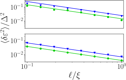
Figure B.1: Energy variance over mean-free path at fixed $k_{\rm F}$ and $\xi_{0}$. The markers show the numerical results in two dimensions (top) and three dimensions (bottom), with $k_{\rm F}\xi_{0}=50$ (blue triangles) and $k_{\rm F}\xi_{0}=100$ (green circles). The lines correspond to the perturbative results derived in the main text. The scattering phase shifts $\phi_{\uparrow}=-\phi_{\downarrow}$ of the magnetic impurity are chosen such that, in the absence of disorder, a YSR state forms at $\varepsilon/\Delta=0$.

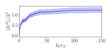
Figure B.2: Convergence of the energy variance with disorder cutoff $r_{N}$ in the dirty limit and in two dimensions. The parameters are $k_{\rm F}\xi_{0}=300$ and $\xi_{0}/\ell=10$, with the same magnetic impurity parameters as in Fig. B.1.

APPENDIX C TRANSFER MATRIX FOR A SINGLE SLICE

In this section we present explicit expressions for the transfer matrix of a thin, disordered and superconducting slice. Using Eq. (37) this enables one to calculate the corresponding scattering matrix of the thin slice.

C.1 Two dimensions

First we consider a two dimensional, circular slice. In this case, we define the radial part of the propagating waves in Eq. (34) as

$$\ket{{\cal R}_{\text{e}m\pm}(r)}=\sqrt{\frac{k_{\rm F}}{4v_{\rm F}}}H_{m}^{(\pm)}(k_{\rm F}r)\begin{pmatrix}1\\ 0\end{pmatrix},$$ (51)

for electrons and

$$\ket{{\cal R}_{\text{h}m\pm}(r)}=\sqrt{\frac{k_{\rm F}}{4v_{\rm F}}}H_{m}^{(\mp)}(k_{\rm F}r)\begin{pmatrix}0\\ 1\end{pmatrix},$$ (52)

for holes.

Within first order Born approximation, for a slice of width $\rm{d}r$, at an energy $\varepsilon$ and at a radius $r_{n}$ from the origin, we obtain the transfer matrix

$${\cal T}^{(n)}_{\nu^{\prime}\nu}=\bra{{\cal R}_{\nu^{\prime}}(r_{n})}\\ \mathrm{d}\hat{T}^{(n)}\delta_{m^{\prime},m}+\mathrm{d}\hat{\Gamma}_{m^{\prime},\,m}^{(n)}\ket{{\cal R}_{\nu}(r_{n})},$$ (53)

with the same multi-index $\nu$ as in the main text. The term diagonal in angular momentum reads

$$\mathrm{d}\hat{T}^{(n)}=(\Delta\tau_{x}-\epsilon)2\pi r_{n}{\rm d}r.$$ (54)

For the disorder element we get

$$\mathrm{d}\hat{\Gamma}_{m^{\prime},\,m}^{(n)}=\sqrt{\gamma 2\pi r_{n}\mathrm{d}r}X_{m^{\prime}-m}^{(n)}\tau_{z}.$$ (55)

The random part is absorbed into

$$X_{m^{\prime}-m}^{(n)}=\begin{cases}Y_{0}^{(n)}&\text{for }\text{m=m'}\\ \frac{Y_{|m^{\prime}-m|}^{(n)}+i\mathrm{sign}(m^{\prime}-m)Z_{|m^{\prime}-m|}^{(n)}}{\sqrt{2}}&\text{else}\end{cases}$$ (56)

corresponding to the Fourier transform of white noise. Here $Y_{m}^{(n)}$ and $Z_{m}^{(n)}$ are independent, normally distributed random variables with zero mean and variance one. Note that not all elements of $X^{(n)}$ are independent since $X_{m^{\prime}-m}=X_{m-m^{\prime}}^{*}$.

C.2 Three dimensions

Next we calculate the transfer matrix of a thin, spherical slice in three dimensions. In this case, the radial modes are defined as

$$\ket{{\cal R}_{\text{e}m\pm}(r)}=\sqrt{\frac{k_{\rm F}^{2}}{4\pi v_{\rm F}}}h_{l}^{(\pm)}(k_{\rm F}r)\begin{pmatrix}1\\ 0\end{pmatrix}$$ (57)

for electrons and

$$\ket{{\cal R}_{\text{h}m\pm}(r)}=\sqrt{\frac{k_{\rm F}^{2}}{4\pi v_{\rm F}}}h_{l}^{(\mp)}(k_{\rm F}r)\begin{pmatrix}0\\ 1\end{pmatrix}$$ (58)

for holes, with a total angular momentum quantum number $l$.

Within first order Born approximation and for a spherical slice of width ${\rm d}r$ at a radius $r_{n}$, the transfer matrix reads

$${\cal T}^{(n)}_{\nu^{\prime}\nu}=\bra{{\cal R}_{\nu^{\prime}}(r_{n})}\\ \mathrm{d}\hat{T}^{(n)}\delta_{l^{\prime}l}\delta_{m^{\prime}m}+\mathrm{d}\hat{\Gamma}_{l^{\prime}m^{\prime}lm}^{(n)}\ket{{\cal R}_{\nu}(r_{n})}$$ (59)

similar to Eq. (53).

The term diagonal in the angular momentum quantum numbers reads

$${\rm d}\hat{T}^{(n)}=(\Delta\tau_{x}-\varepsilon)4\pi r_{n}^{2}{\rm d}r$$ (60)

and the disorder element is

$$\mathrm{d}\hat{\Gamma}_{l^{\prime}m^{\prime}lm}^{(n)}=\tau_{z}\sqrt{\gamma 4\pi r_{n}^{2}{\rm d}r}\Xi_{l^{\prime}m^{\prime}lm}.$$ (61)

The random variable $\Xi_{l^{\prime}m^{\prime}lm}$ takes a more complicated form in three than in two dimensions, due to the involvement of the product of two spherical harmonics in the calculation of the matrix elements in Eq. (38). These products can be expressed as a sum over single spherical harmonics for which explicit expressions are known Varshalovich et al. (1988). For these single spherical harmonics we can calculate the overlap with the Gaussian disorder potential. Following this strategy we obtain

$$\Xi_{l^{\prime}m^{\prime}lm}=\sum_{L=0}^{\infty}c^{L,\,\Delta m}_{l^{\prime}m^{\prime}lm}X_{L,\,\Delta m}$$ (62)

where the coefficients for the transformation between a single and the product of two spherical harmonics are

$$c^{L,\,\Delta m}_{l^{\prime}m^{\prime}lm}= (-1)^{m}\sqrt{\frac{(2l^{\prime}+1)(2l+1)}{4\pi(2L+1)}}$$ (63)

$$\times C_{l^{\prime},\,0,\,l,\,0}^{L,\,0}C_{l^{\prime},\,m^{\prime},\,l,\,m}^{L,\,\Delta m}.$$ (64)

Here

$$C_{l^{\prime},\,m^{\prime},\,l,\,m}^{L,\,\Delta m}=\braket{l^{\prime},\,m^{\prime},\,l,\,m}{L,\,\Delta m}$$ (65)

are the Clebsch Gordan coefficients Varshalovich et al. (1988). Additionally, the overlap of the single spherical harmonics with the angular part of the Gaussian disorder potential yields the random numbers Lang and Schwab (2015)

$$X_{L,\,\Delta m}^{(n)}=\begin{cases}\frac{Y_{L,\,\Delta m}^{(n)}+iZ_{L,\,\Delta m}^{(n)}}{\sqrt{2}}&\text{for }\Delta m>0\\ Y_{L,\,0}^{(n)}&\text{for }\Delta m=0\\ (-1)^{\Delta m}X_{L,\,-\Delta m}^{(n)}&\text{for }\Delta m<0\end{cases}$$ (66)

Here, similar to the two dimensional case, $Y_{L,\,\Delta m}$ and $Z_{L,\,\Delta m}$ are independent, normally distributed random variables with zero mean and variance one.

References

- Yu (1965) L. Yu, Acta Phys. Sin. 21, 75 (1965).
- Shiba (1968) H. Shiba, Prog. Theor. Phys. 40, 435 (1968).
- Rusinov (1968) A. I. Rusinov, Zh. Eksp. Teor. Fiz. Pisma Red. 9, 146 (1968), [JETP Lett. 9, 85 (1969)].
- Rusinov (1969) A. I. Rusinov, Zh. Eksp. Teor. Fiz. Pisma Red. 56, 2047 (1969), [JETP Lett. 29, 1101 (1969)].
- Zittartz et al. (1972) J. Zittartz, A. Bringer, and E. Müller-Hartmann, Solid State Commun. 10, 513 (1972).
- Hirschfeld et al. (1988) P. J. Hirschfeld, P. Wölfle, and D. Einzel, Phys. Rev. B 37, 83 (1988).
- Balatsky et al. (2006) A. V. Balatsky, I. Vekhter, and J.-X. Zhu, Rev. Mod. Phys. 78, 373 (2006).
- Morr and Y. (2006) D. K. Morr and J. Y., Phys. Rev. B 73, 224511 (2006).
- Moca et al. (2008) C. P. Moca, E. Demler, B. Jankó, and G. Zaránd, Phys. Rev. B 77, 174516 (2008).
- Žitko et al. (2011) R. Žitko, O. Bodensiek, and T. Pruschke, Phys. Rev. B 83, 054512 (2011).
- Yao et al. (2014) N. Yao, L. Glazman, E. Demler, M. Lukin, and J. Sau, Phys. Rev. Lett. 113, 087202 (2014).
- Hoffman et al. (2015) S. Hoffman, J. Klinovaja, T. Meng, and D. Loss, Phys. Rev. B 92, 125422 (2015).
- Kim et al. (2015) Y. Kim, J. Zhang, E. Rossi, and R. M. Lutchyn, Phys. Rev. Lett. 114, 236804 (2015).
- Meng et al. (2015) T. Meng, J. Klinovaja, S. Hoffman, P. Simon, and D. Loss, Phys. Rev. B 92, 064503 (2015).
- Žitko (2016) R. Žitko, Phys. Rev. B 93, 195125 (2016).
- Yazdani et al. (1997) A. Yazdani, B. A. Jones, C. P. Lutz, M. F. Crommie, and D. M. Eigler, Science 275, 1767 (1997).
- Ji et al. (2008) S.-H. Ji, T. Zhang, Y.-S. Fu, X. Chen, X.-C. Ma, J. Li, W.-H. Duan, J.-F. Jia, and Q.-K. Xue, Phys. Rev. Let. 100, 226801 (2008).
- Ji et al. (2010) S.-H. Ji, T. Zhang, Y.-S. Fu, X. Chen, J.-F. Jia, Q.-K. Xue, and X.-C. Ma, Appl. Phys. Let. 96, 073113 (2010).
- Franke et al. (2011) K. J. Franke, G. Schulze, and J. I. Pascual, Science 332, 940 (2011).
- Ménard et al. (2015) G. C. Ménard, S. Guissart, C. Brun, S. Pons, V. S. Stolyarov, F. Debontridder, M. V. Leclerc, E. Janod, L. Cario, D. Roditchev, P. Simon, and T. Cren, Nat. Phys. 11, 1013 (2015).
- Ruby et al. (2015a) M. Ruby, F. Pientka, Y. Peng, F. von Oppen, B. W. Heinrich, and K. J. Franke, Phys. Rev. Lett. 115, 087001 (2015a).
- Hatter et al. (2015) N. Hatter, B. W. Heinrich, M. Ruby, J. I. Pascual, and K. J. Franke, Nat. Commun. 6, 8988 (2015).
- Ruby et al. (2016) M. Ruby, Y. Peng, F. von Oppen, B. W. Heinrich, and K. J. Franke, Phys. Rev. Lett. 117, 186801 (2016).
- Choi et al. (2016) D.-J. Choi, C. Rubio-Verdú, J. de Bruijckere, M. Moreno Ugeda, N. Lorente, and J. I. Pascual, arXiv:1608.03752 (2016).
- Kezilebieke et al. (2017) S. Kezilebieke, M. Dvorak, T. Ojanen, and P. Liljeroth, arXiv:1701.03288 (2017).
- Heinrich et al. (2017) B. W. Heinrich, J. I. Pascual, and K. J. Franke, arXiv:1705.03672 (2017).
- Nadj-Perge et al. (2014) S. Nadj-Perge, I. K. Drozdov, J. Li, H. Chen, S. Jeon, J. Seo, A. H. MacDonald, B. A. Bernevig, and A. Yazdani, Science 346, 602 (2014).
- Ruby et al. (2015b) M. Ruby, F. Pientka, Y. Peng, F. von Oppen, B. W. Heinrich, and K. J. Franke, Phys. Rev. Lett. 115, 197204 (2015b).
- Pawlak et al. (2016) R. Pawlak, M. Kisiel, J. Klinovaja, T. Meier, S. Kawai, T. Glatzel, D. Loss, and E. Meyer, Npj Quantum Information 2, 16035 (2016).
- Feldman et al. (2017) B. E. Feldman, M. T. Randeria, J. Li, S. Jeon, Y. Xie, Z. Wang, I. K. Drozdov, B. Andrei Bernevig, and A. Yazdani, Nat. Phys. 13, 286 (2017).
- Ruby et al. (2017) M. Ruby, B. W. Heinrich, Y. Peng, F. von Oppen, and K. J. Franke, arXiv:1704.05756 (2017).
- Kitaev (2003) A. Kitaev, Annals of Physics 303, 2 (2003).
- Nayak et al. (2008) C. Nayak, S. H. Simon, A. Stern, M. Freedman, and S. Das Sarma, Rev. Mod. Phys. 80, 1083 (2008).
- Nadj-Perge et al. (2013) S. Nadj-Perge, I. K. Drozdov, B. A. Bernevig, and A. Yazdani, Phys. Rev. B 88, 020407 (2013).
- Pientka et al. (2013) F. Pientka, L. I. Glazman, and F. von Oppen, Phys. Rev. B 88, 155420 (2013).
- Klinovaja et al. (2013) J. Klinovaja, P. Stano, A. Yazdani, and D. Loss, Phys. Rev. Lett. 111, 186805 (2013).
- Braunecker and Simon (2013) B. Braunecker and P. Simon, Phys. Rev. Lett. 111, 147202 (2013).
- Kim et al. (2014) Y. Kim, M. Cheng, B. Bauer, R. M. Lutchyn, and S. Das Sarma, Phys. Rev. B 90, 060401 (2014).
- Schecter et al. (2016) M. Schecter, K. Flensberg, M. H. Christensen, B. M. Andersen, and J. Paaske, Phys. Rev. B 93, 140503 (2016).
- Hui et al. (2015) H.-Y. Hui, J. D. Sau, and S. D. Sarma, Phys. Rev. B 92, 174512 (2015).
- Clogston (1962) A. M. Clogston, Phys. Rev. 125, 439 (1962).
- (42) Eq. (10) assumes that the range of the impurity potential satisfies the inequality . If , a correction to Eq. (10) in the form of a Cauchy principal value integral has to be included into Eq. (10), see Ref. Clogston, 1962. Since we express our results in terms of the phase shifts , these corrections are not important for our considerations.
- Pientka et al. (2015) F. Pientka, Y. Peng, L. Glazman, and F. von Oppen, Physica Scripta 2015, 014008 (2015).
- Pientka et al. (2014) F. Pientka, L. I. Glazman, and F. von Oppen, Phys. Rev. B 89, 180505 (2014).
- Varshalovich et al. (1988) D. A. Varshalovich, A. N. Moskalev, and V. K. Khersonskii, Quantum theory of angular momentum (World scientific, 1988).
- Lang and Schwab (2015) A. Lang and C. Schwab, Ann. Appl. Probab. 25, 3047 (2015).