Topological lattice using multi-frequency radiation

Abstract

We describe a novel technique for creating an artificial magnetic field for ultra-cold atoms using a periodically pulsed pair of counter propagating Raman lasers that drive transitions between a pair of internal atomic spin states: a multi-frequency coupling term. In conjunction with a magnetic field gradient, this dynamically generates a rectangular lattice with a non-staggered magnetic flux. For a wide range of parameters, the resulting Bloch bands have non-trivial topology, reminiscent of Landau levels, as quantified by their Chern numbers.

1 Introduction

Ultracold atoms find wide applications in realising condensed matter phenomena [1, 2, 3, 4]. Since ultracold atom systems are ensembles of electrically neutral atoms, various methods have been used to simulate Lorentz-type forces, with an eye for realizing physics such as the quantum Hall effect (QHE). Lorentz forces are present in spatially rotating systems [5, 6, 7, 8, 9, 10, 11] and appear in light-induced geometric potentials [12, 13]. The magnetic fluxes achieved with these methods are not sufficiently large for realizing the integer or fractional QHE. In optical lattices, larger magnetic fluxes can be created by shaking the lattice potential [14, 15, 16, 17], combining static optical lattices along with laser-assisted spin or pseudo spin coupling [18, 19, 20, 12, 21, 22, 13, 23, 24]; current realizations of these techniques are beset with micro motion and interaction induced heating effects. Here we propose a new method that simultaneously creates large artificial magnetic fields and a lattice that may overcome these limitations.

Our technique relies on a pulsed atom-light coupling between internal atomic states along with a state-dependent gradient potential that together create a two-dimensional (2D) periodic potential with an intrinsic artificial magnetic field. With no pre-existing lattice potential, there are no a priori resonant conditions that would otherwise constrain the modulation frequency to avoid transitions between original Bloch bands [25]. For a wide range of parameters, the ground and excited bands of our lattice are topological, with nonzero Chern number. Moreover, like Landau levels the lowest several bands can all have unit Chern number.

The manuscript is organized as follows. Firstly, we describe a representative experimental implementation of our technique directly suitable for alkali atoms. Secondly, because the pulsed atom-light coupling is time-periodic, we use Floquet methods to solve this problem. Specifically, we employ a stroboscopic technique to obtain an effective Hamiltonian. Thirdly, using the resulting band structure we obtain a phase diagram which includes a region of Landau level-like bands each with unit Chern number.

2 Pulsed lattice

Figure 1 depicts a representative experimental realization of the proposed method. A system of ultracold atoms is subjected to a magnetic field with a strength $B(X)=B_{0}+B^{\prime}X$. This induces a position-dependent splitting $g_{F}\mu_{{\rm B}}B$ between the spin up and down states; $g_{F}$ is the Land $g$-factor and $\mu_{{\rm B}}$ is the Bohr magneton. Additionally, the atoms are illuminated by a pair of Raman lasers counter propagating along ${\bf e}_{y}$, i.e. perpendicular to the detuning gradient. The first beam (up-going in Fig. 1(a)) is at frequency $\omega^{+}=\omega_{0}$, while the second (down-going in Fig. 1(a)) contains frequency components $\omega_{n}^{-}=\omega_{0}+(-1)^{n}(\delta\omega+n\omega)$; the difference frequency between these beams contains frequency combs centered at $\pm\delta\omega$ with comb teeth spaced by $2\omega$, as shown in Fig. 1(b). In our proposal, the Raman lasers are tuned to be in nominal two-photon resonance with the Zeeman splitting from the large offset field $B_{0}$ such that $g_{F}\mu_{{\rm B}}B_{0}=\hbar\delta\omega_{0}$, making the frequency difference $\omega_{n=0}^{-}-\omega^{+}$ resonant at $X=0$, where $B=B_{0}$. Intuitively, each additional frequency component $\omega_{n}^{-}$ adds a resonance condition at the regularly spaced points $X_{n}=n\hbar\omega/g_{F}\mu_{{\rm B}}B^{\prime}$, however, transitions using even-$n$ side bands give a recoil kick opposite from those using odd-$n$ side bands (see Fig. 1(c)). Each of these coupling-locations locally realizes synthetic magnetic field experiment performed at the National Institute of Standards and Technology (NIST) [26], arrayed in a manner to give a rectified artificial magnetic field with a non-zero average that we will show is a novel flux lattice.

In practice only a finite number of lattice teeth are needed, owing to the finite spatial extent of a trapped atomic gas. In rough numbers the spatial extent of a quantum degenerate gas is about $20\mu m$, and if we select a very large gradient corresponding to a lattice spacing of $0.5\mu m$, this gives just 40 comb teeth. Note also that generating the frequency comb is a very straightforward procedure. In the laboratory one uses acoustic-optical modulators (AOMs) to frequency shift laser beams by a frequency defined by a laboratory radiofrequency (rf) source. Therefore creating a comb is a simple matter of first creating a frequency comb – simple with rf – and then feeding that signal into the AOM. This sort of frequency synthesis is being carried in a routine manner in the ultracold atom labs.

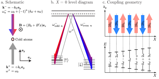
Figure 1: Floquet flux lattice. a. Experimental schematic depicting a cold cloud of atoms in a gradient magnetic field, illuminated by a pair of counter-propagating laser beams tuned near two-photon Raman resonance. The down-going beam includes sidebands both to the red and blue of the carrier ($\omega_{0}$) in resonance at different spatial positions along ${\bf e}_{x}$. b. Level diagram showing even and odd side-bands linking the $\left|\uparrow\right\rangle$ and $\left|\downarrow\right\rangle$ states with differing detuning from resonance at $X=0$. c. Spatially dependent coupling. Bottom: different frequency components are in two-photon resonance in different $X$ positions. Top: the recoil kick associated with the Raman transition is along $\pm\mathbf{e}_{y}$ and thus alternates spatially depending on whether the Raman transition is driven from the red or blue sideband of the down-going laser beam.

We formally describe our system by first making the rotating wave approximation (RWA) with respect to the large offset frequency $\omega_{0}$. This situation is modeled in terms of a spin-1/2 atom of mass $M$ and wave-vector $\bm{K}=-i\bm{\nabla}$ with a Hamiltonian

$$H(t)=H_{0}+V(t).$$ (1)

The first term is

$$H_{0}=\frac{\hbar^{2}\bm{K}^{2}}{2M}+\frac{\Delta(X)}{2}\sigma_{3},$$ (2)

where $\Delta(X)=\Delta^{\prime}X$ describes the detuning gradient along $\mathbf{e}_{x}$ axis, and $\sigma_{3}=|\!\uparrow\rangle\langle\uparrow\!|-|\!\downarrow\rangle\langle\downarrow\!|$ is a Pauli spin operator. In the RWA only near-resonant terms are retained, giving the Raman coupling described by

$$V(t)=V_{0}\sum_{n}\left[{\rm e}^{{\rm i}(K_{0}Y-2n\omega t)}+{\rm e}^{{\rm i}(-K_{0}Y-(2n+1)\omega t)}\right]|\!\downarrow\rangle\langle\uparrow\!|+{\rm H.\,c.}\,.$$ (3)

The first term describes coupling from the sidebands with even frequencies $2n\omega$, whereas the second term describes coupling from the sidebands with odd frequencies $\left(2n+1\right)\omega$. The recoil kick is aligned along $\pm\mathbf{e}_{y}$ with opposite sign for the even and odd frequency components. In writing Eq.(3) we assumed that the coupling amplitude $V_{0}$ and the associated recoil wave number $K_{0}$ are the same for all frequency components. The coupling Hamiltonian $V(t)$ and therefore the full Hamiltonian $H(t)$ are time-periodic with period $2\pi/\omega$, and we accordingly apply Floquet techniques.

3 Theoretical analysis

The outline of this Section is as follows. (1) We begin the analysis of the Hamiltonian given by Eq. (1) by moving to dimensionless units; (2) subsequently derive an approximate effective Hamiltonian from the single-period time evolution operator; (3) provide an intuitive description in terms of adiabatic potentials; and (4) finally solve the band structure, evaluate its topology and discuss possibilities of the experimental implementation.

3.1 Dimensionless units

For the remainder of the manuscript we will use dimensionless units. All energies will be expressed in units of $\hbar\omega$, derived from the Floquet frequency $\omega$; time will be expressed in units of inverse driving frequency $\omega^{-1}$, denoted by $\tau=\omega t$; spatial coordinates will be expressed in units of inverse recoil momentum $K_{0}^{-1}$, denoted by lowercase letters $(x,y)=K_{0}(X,Y)$. In these units, the Hamiltonian (1) takes the form

$$h(\tau)=\frac{H(\tau/\omega)}{\hbar\omega}=E_{\rm{r}}\bm{k}^{2}+\frac{1}{2}\bm{\Omega}(\tau)\cdot\bm{\sigma}\,,$$ (4)

where $E_{\rm{r}}=\hbar^{2}K_{0}^{2}/(2M\hbar\omega)$ is the dimensionless recoil energy associated with the recoil wavenumber $K_{0}$; $\bm{k}=\bm{K}/K_{0}$ is the dimensionless wavenumber. The dimensionless coupling

$$\bm{\Omega}(x,y,\tau)=\left(2{\rm Re}\,u(y,\tau),\,2{\rm Im}\,u(y,\tau),\,\beta x\right)$$ (5)

includes a combination of position-dependent detuning and Raman coupling. Here $\beta=\Delta^{\prime}/(\hbar\omega k_{0})$ describes the linearly varying detuning in dimensionless units; the function $u(y,\tau)=v_{0}\sum_{n}\left\{\exp[{\rm i}(y-2n\tau)]+\exp[{\rm i}(-y-(2n+1)\tau)]\right\}$ is a dimensionless version of the sum in Eq. (3) with $v_{0}=V_{0}/(\hbar\omega)$.

In the time domain the coupling given by Eq. (5) is

$$\frac{1}{2}\bm{\Omega}(\tau)\cdot\bm{\sigma}=\frac{1}{2}\beta x\sigma_{3}+\sum_{l}v_{l}(y)\delta(\tau-\pi l),$$ (6)

with

$$v_{l}(y)=\pi v_{0}\left[{\rm e}^{{\rm i}y}+(-1)^{l}{\rm e}^{-{\rm i}y}\right]|\!\downarrow\rangle\langle\uparrow\!|+{\rm H.\,c.}\,.$$ (7)

In this way we have separated the spatial and temporal dependencies in the coupling (6).

3.2 Effective Hamiltonian

We continue our analysis by deriving an approximate Hamiltonian that describes the complete time evolution over a single period from $\tau=0-\epsilon$ to $\tau=2\pi-\epsilon$ with $\epsilon\to 0$. This evolution includes a kick $v_{0}$ at the beginning of the period $\tau_{+}=0$ and a second kick $v_{1}$ in the middle of the period $\tau_{-}=\pi$; between the kicks the evolution includes the kinetic and gradient energies. In the full time period, the complete evolution operator is a product of four terms:

$$U(2\pi,0)\equiv\lim_{\epsilon\to 0}U(2\pi-\epsilon,0-\epsilon)=U_{0}U_{\rm{kick}}^{(1)}U_{0}U_{\rm{kick}}^{(0)}.$$ (8)

Here

$$U_{0}=\exp\left\{-{\rm i}\pi\left[E_{\rm{r}}\bm{k}^{2}+\frac{1}{2}\sigma_{3}\beta x\right]\right\}$$ (9)

is the evolution operator over a half period, generated by kinetic energy and gradient. The operator

$$U_{\rm{kick}}^{(l)}=\exp\left[-{\rm i}v_{l}(y)\right].$$ (10)

describes a kick at $\tau=l\pi$.

We obtain an effective Hamiltonian by assuming that the Floquet frequency $\omega$ greatly exceeds the recoil frequency, $1\gg E_{\rm{r}}$, allowing us to ignore the commutators between the kinetic energy and functions of coordinates in eq.(8). We then rearrange terms in the full time evolution operator (8) and obtain (see Appendix A)

$$U_{\rm{eff}}=\exp\left\{-{\rm i}2\pi\left[E_{\rm{r}}\bm{k}^{2}+v_{\rm{eff}}\right]\right\},$$ (11)

where $v_{\rm{eff}}$ is an effective coupling defined by

$$\exp\left(-{\rm i}2\pi v_{\rm{eff}}\right)={\rm e}^{-{\rm i}\pi\sigma_{3}\beta x/2}U_{\rm{kick}}^{(1)}{\rm e}^{-{\rm i}\pi\sigma_{3}\beta x/2}U_{\rm{kick}}^{(0)}.$$ (12)

The function $v_{l}(y)$ entering the kick operators $U_{\rm{kick}}^{(l)}$ is spatially periodic along the $y$ direction with a period $2\pi$. This period can be halved to $\pi$ by virtue of a gauge transformation $U=\exp(-{\rm i}y\sigma_{3}/2)$. Subsequently, when exploring energy bands and their topological properties, this prevents problems arising from using a twice larger elementary cell. Following this transformation the evolution operator becomes

$$U_{\rm{eff}}=\exp\left\{-{\rm i}2\pi\left[E_{\rm{r}}\left(\bm{k}+\sigma_{3}\bm{e}_{y}/2\right)^{2}+v_{\rm{eff}}\right]\right\},$$ (13)

where $v_{l}(y)$ featured in the kick operators $U_{\rm{kick}}^{(l)}$ has now the spatial periodicity $\pi$ along the $y$ direction, i.e. it should be replace to

$$v_{l}(y)=\pi v_{0}\left[{\rm e}^{{\rm i}2y}+(-1)^{l}\right]|\!\downarrow\rangle\langle\uparrow\!|+{\rm H.\,c.}\,.$$ (14)

The algebra of Pauli matrices allows us to write the effective coupling $v_{\rm{eff}}(\bm{r})$ featured in the evolution equations (12)-(13) as:

$$v_{\rm{eff}}(\bm{r})=\frac{1}{2}\bm{\Omega}_{\rm{eff}}(\bm{r})\cdot\bm{\sigma},$$ (15)

where $\bm{\Omega}_{\rm{eff}}=\left(\Omega_{\rm{eff},1},\Omega_{\rm{eff},2},\Omega_{\rm{eff},3}\right)$ is a position-dependent effective Zeeman field which takes the analytic form

$$\exp\left(-{\rm i}2\pi v_{\rm{eff}}\right)=q_{0}-{\rm i}q_{1}\sigma_{1}-{\rm i}q_{2}\sigma_{2}-{\rm i}q_{3}\sigma_{3}.$$ (16)

Here $q_{0}$, $q_{1}$, $q_{2}$ and $q_{3}$ are real functions of the coordinates $(x,y)$, allowing to express the effective Zeeman field as

$$\bm{\Omega}_{\rm{eff}}=\pi^{-1}\frac{\bm{q}}{||\bm{q}||}\arccos q_{0},$$ (17)

where $\bm{q}$ is a shorthand of a three dimensional vector $(q_{1},q_{2,}q_{3})$. In general the equation (16) gives multiple solutions that correspond for different Floquet bands. Our choice (17) picks only to the two bands that lie in the energy window from $-1/2$ to $1/2$ covering a single Floquet period.

Comparing (12) and (16) and multiplying four matrix exponents give explicit expressions

$$q_{0} =\cos f_{1}\cos f_{2}\cos(\pi\beta x),$$ (18)

$$q_{1} =\sin f_{1}\cos f_{2}\cos(y+\pi\beta x)-\cos f_{1}\sin f_{2}\sin(y),$$ (19)

$$q_{2} =\sin f_{1}\cos f_{2}\sin(y+\pi\beta x)+\cos f_{1}\sin f_{2}\cos(y),$$ (20)

$$q_{3} =\cos f_{1}\cos f_{2}\sin(\pi\beta x)-\sin f_{1}\sin f_{2}$$ (21)

with

$$f_{1}(y) =2\pi v_{0}\cos(y),$$ (22)

$$f_{2}(y) =2\pi v_{0}\sin(y).$$ (23)

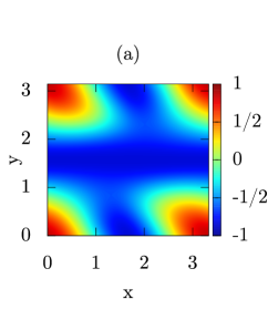
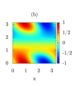
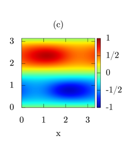
Figure 2: Coupling components (a) $\Omega_{\rm{eff},1}(\bm{r})$, (b) $\Omega_{\rm{eff},2}(\bm{r})$ and (c) $\Omega_{\rm{eff},3}(\bm{r})$ for $v_{0}=0.25$ and $\beta=0.6$ calculated using Eqs. (17)-(23). The corresponding eigenvalues of the coupling $v_{\pm}(\bm{r})=\pm\Omega_{\rm{eff}}/2$ are presented by the thick red solid lines in the fig. 3.

These explicit expressions show that the resulting effective Zeeman field (17) and the associated effective coupling (15) are periodic along both $\bm{e}_{x}$ and $\bm{e}_{y}$, with spatial periods $a_{x}=2/\beta$ and $a_{y}=\pi$ respectively. Therefore, although the original Hamiltonian containing the spin-dependent potential slope $\propto x\sigma_{3}$ is not periodic along the $x$ direction, the effective Floquet Hamiltonian is. The spatial dependence of the Zeeman field components $\Omega_{\rm{eff},1}$, $\Omega_{\rm{eff},2}$ and $\Omega_{\rm{eff},3}$ is presented in the fig. 2 for $\beta=0.6$ giving an approximately square unit cell. In fig. 2 we select $v_{0}=0.25$ where the absolute value of the Zeeman field $\Omega_{\rm{eff}}$ is almost uniform, as is apparent from the nearly flat adiabatic bands shown in fig. 3 below.

3.3 Adiabatic evolution and magnetic flux

Before moving further to an explicit numerical analysis of the band structure, we develop an intuitive understanding by performing an adiabatic analysis of motion governed by effective Hamiltonian

$$h_{\rm{eff}}(\bm{r})=E_{\rm{r}}\left(\bm{k}+\sigma_{3}\bm{e}_{y}/2\right)^{2}+\frac{1}{2}\bm{\Omega}_{\rm{eff}}\cdot\bm{\sigma}\,$$ (24)

featured in the evolution operator $U_{\rm{eff}}$, Eq. (11). The coupling field $\bm{\Omega}_{\rm{eff}}(\bm{r})$ is parametrized by the spherical angles $\theta(\bm{r})$ and $\phi(\bm{r})$ defined by

$$\cos\theta =\frac{\Omega_{\rm{eff},3}}{\Omega_{\rm{eff}}},$$ (25)

$$\tan\phi =\frac{\Omega_{\rm{eff},2}}{\Omega_{\rm{eff},1}}.$$ (26)

This gives the effective coupling [12]

$$\frac{1}{2}\bm{\Omega}_{\rm{eff}}\cdot\bm{\sigma}=\frac{1}{2}\Omega_{\rm{eff}}\left[\begin{array}[]{cc}\cos\theta&{\rm e}^{-{\rm i}\phi}\sin\theta\\ {\rm e}^{{\rm i}\phi}\sin\theta&-\cos\theta\end{array}\right]\,,$$ (27)

characterized by the position-dependent eigenstates

$$\left|+\right\rangle=\left(\begin{array}[]{c}\cos\left(\theta/2\right)\\ {\rm e}^{{\rm i}\phi}\sin\left(\theta/2\right)\end{array}\right)\,,\qquad\left|-\right\rangle=\left(\begin{array}[]{c}-{\rm e}^{-{\rm i}\phi}\sin\left(\theta/2\right)\\ \cos\left(\theta/2\right)\end{array}\right)\,.$$ (28)

The corresponding eigenvalues

$$v_{\pm}(\bm{r})=\pm\frac{1}{2}\Omega_{\rm{eff}},$$ (29)

are shown in Fig. 3 for various value of the Raman coupling $v_{0}$. As one can see in Fig. 3, for $v_{0}=0.25$ the resulting bands $v_{\pm}(\bm{r})$ (adiabatic potentials) are flat and have a considerable gap $\approx\omega/2$, a regime suitable for a description in terms of an adiabatic motion in selected bands [27].

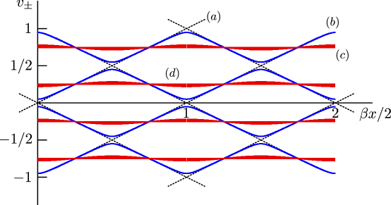
Figure 3: Adiabatic Floquet potentials given by Eq. (29) for $\beta=0.6$ us. (a) Thin black dotted lines denote the spin-dependent gradient slopes without including the Raman coupling ($v_{0}=0$); (b) thin blue solid lines denote effective adiabatic potentials for weak Raman coupling ($v_{0}=0.05$) (c) red solid lines denote nearly flat adiabatic potentials that are achieved for stronger Raman coupling ($v_{0}=0.25$). All the curves are projected into $x$ plane for various $y$ values. A weak $y$ dependence of the adiabatic potentials is seen to appear in the strong coupling case (c) making the superimposed red lines thicker.

As in Ref. [28], we consider the adiabatic motion of the atom in one of these flat adiabatic bands with the projection Shr dinger equation that includes a geometric vector potential

$$\bm{A}_{\pm}(\bm{r})=\pm\frac{1}{2}\left(\cos\theta-1\right)\nabla\phi\,.$$ (30)

This provides a synthetic magnetic flux density $\bm{B}_{\pm}(\bm{r})=\nabla\times\bm{A}_{\pm}(\bm{r})$. The geometric vector potential $\bm{A}_{\pm}(\bm{r})$ may contain Aharonov-Bohm type singularities, that give rise to a synthetic magnetic flux over an elementary cell

$$\alpha_{\pm}=-\sum\oint_{{\rm singul}}{\rm d}\bm{r}\cdot\bm{A}_{\pm}(\bm{r}).$$ (31)

The singularities appear at points where $\theta=\pi$, where the angle $\phi$ and its gradient $\nabla\phi$ are undefined and $\cos\theta=-1$. The term $\cos\theta-1$ in (30) is non zero and does not remove the undefined phase $\nabla\phi$. Our unit cell contains two such singularities located at $\bm{r}=(a_{x},3a_{y})/4$ and $\bm{r}=(3a_{x},a_{y})/4$, containing the same flux, so that they do not compensate each other, giving the synthetic magnetic flux $\pm 2\pi$ in each unit cell. Note that usually the optical lattices are sufficiently deep, and the $\pm 2\pi$ flux per elementary is topologically trivial. In that case the tight binding model can be applied, with the tunneling taking place only between the nearest-neighboring sites of the square plaquette. The $\pm 2\pi$ flux over the square plaquette can then be eliminated by a gauge transformation. Yet if the lattice is shallow enough, the tight binding model is not applicable and the above arguments do not work. In the present situation, the most interesting topological lattice appears for a flat adiabatic trapping potential shown by a solid red curve in Fig. 3. In such a situation there are no well defined lattice sites, and the $\pm 2\pi$ flux per elementary cell results in topologically non-trivial bands explored in the next Subsection.

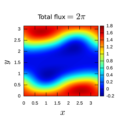
Figure 4: Geometric flux density $\bm{B}_{\pm}(\bm{r})=\nabla\times\bm{A}_{\pm}(\bm{r})$ computed for $v_{0}=0.25$ and $\beta=0.6$ using Eq. (30). The overall spatial structure of this flux density does not depend on the gradient $\beta$; rather it scales with the corresponding lattice constant $a_{x}=2/\beta$.

For a weak coupling (such as $v=0.05$) the geometric flux density $\bm{B}(\bm{r})\equiv\bm{B}_{\pm}(\bm{r})$ is concentrated around the intersection points of the gradient slopes shown in in Fig. 3 and has a very weak $y$ dependence. With increasing the coupling $v$, the flux extends beyond the intersection areas and acquires a $y$ dependence. Fig. 4 shows the geometric flux density $\bm{B}(\bm{r})\equiv\bm{B}_{+}(\bm{r})$ for the strong coupling ($v_{0}=0.25$) corresponding to the most flat adiabatic bands. In this regime the flux develops stripes in the $x$ direction and has a strong $y$ dependence. For the whole range of coupling strengths $0\leq v_{0}\leq 1/2$ the total synthetic magnetic flux per unit cell is $2\pi$ and is independent of the Floquet frequency $\omega$ and the gradient $\beta$.

Now let us discuss the effect of an extra spin-independent trapping potential. The present scheme requires a large spin-dependent energy gradient which would have a huge influence on the relative trapping for the two spin states without the Raman coupling or for a weak Raman coupling. In that case one would expect that the stable positions for any trapped sample of the two spin states would live at entirely distinct locations, possibly with no overlap. Yet we are interested mostly in a sufficiently strong Raman coupling where the two spin states get mixed, and the atomic motion takes place in almost flat adiabatic potentials shown in red in Fig. 3. Therefore the atoms are no longer affected by the steep spin-dependent potential slopes, and the spin-independent trapping potential would not cause separation of different spin states. Instead, the extra spin-independent parabolic trapping potential would simply make the flat adiabatic trapping potentials parabolic. Of course, one needs to be all the time in the regime where the Raman coupling is strong compared to the characteristic energy of the spin-dependent potential slope. That is why we propose to introduce the spin-dependent potential gradient only at the final stage of the adiabatic protocol discussed in Sect. 3.5.

3.4 Band structure and Chern numbers

We analyze the topological properties of this Floquet flux lattice by explicitly numerically computing the band structure and associated Chern number using the effective Hamiltonian (24) without making the adiabatic approximation introduced in Sec. 3.3. Again the gradient of the original magnetic field is such that we approximately get a square lattice, $\beta=0.6$. Furthermore, we choose the Floquet frequency to be ten times larger than the recoil energy, $E_{\rm{r}}=0.1$. Note that one can alter the length of the plaquette along the x direction (and thus the flux density) by changing $\beta$ representing the potential gradient along the $x$ axis.

First, let us consider the case where $v_{0}=0.25$ corresponding to the most flat adiabatic potential. In this situation the Chern numbers of the first five bands appear to be equal to the unity, as one can see in the left part of Fig. 5. Thus the Hall current should monotonically increase when filling these bands. This resembles the Quantum Hall effect involving the Landau levels. Second, we check what happens when we leave the regime $v_{0}=0.25$ where the adiabatic potential is flat, and consider lower and higher values of the coupling strength $v_{0}$. Near $v_{0}=0.175$ we find a topological phase transition where the lowest two energy bands touch and their Chern numbers change to $c_{1}=0$ and $c_{2}=2$, while the Chern numbers of the higher bands remain unchanged, illustrated in fig. 6. In a vicinity of $v_{0}=0.3$ there is another phase transition, where the second and third bands touch, leading to a new distribution of Chern numbers: $c_{1}=1$, $c_{2}=-1$, $c_{3}=3$, $c_{4}=1$. Interestingly the Chern numbers of the second and the third bands jump by two units during such a transition.

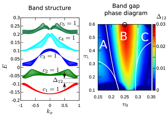
Figure 5: Left: band structure calculated using the effective Hamiltonian (24) for $v_{0}=0.25$, $\beta=0.6$ and $E_{\rm{r}}=0.1$. Right: The band gap $\Delta_{12}$ between the first and second bands for $E_{\rm{r}}=0.1$ and various values of $v_{0}$ and $\beta$.

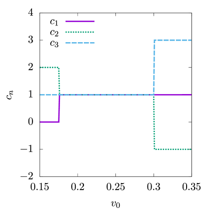
Figure 6: Dependence of Chern number for the bands calculated using the effective Hamiltonian (24) on the coupling strength $v_{0}$ for $\beta=0.6$ and $E_{\rm{r}}=0.1$. Here we present the Chern numbers $c_{1}$, $c_{2}$ and $c_{3}$ of the three lowest bands.

Finally, we explore the robustness of the topological bands. The right part of Fig. 5 shows the dependence of the band gap $\Delta_{12}$ between the first and second bands on the coupling strength $v_{0}$ and the potential gradient $\beta$. One can see that the band gap is maximum for $v_{0}=0.25$ when the adiabatic potential is the most flat. The gap increases by increasing the gradient $\beta$, simultaneously extending the range of the $v_{0}$ values where the band gap is nonzero. Therefore to observe the topological bands, one needs to take a proper value of the Raman coupling $v_{0}\approx 0.25$ and a sufficiently large gradient $\beta$, such as $\beta=0.6$.

We now make some numerical estimates to confirm that this scheme is reasonable. We consider an ensemble of ${}^{87}{\rm Rb}$ atoms, with $\left|{\uparrow}\right>=\left|f=2,m_{F}=2\right>$ and $\left|\downarrow\right>=\left|{f=1,m_{F}=1}\right>$; the relative magnetic moment of these hyperfine states is $\approx 2.1\ {\rm MHz}/{\rm G}$, where $1\ {\rm G}=10^{-4}\ {\rm T}$. For a reasonable magnetic field gradient of $300\ \mathrm{G}/\mathrm{cm}$, this leads to the $\Delta^{\prime}/\hbar\approx 2\pi\times 600\ \mathrm{MHz}/\mathrm{cm}=2\pi\times 60\ {\rm kHz}/\mu{\rm m}$ detuning gradient. For ${}^{87}{\rm Rb}$ with $\lambda=790\ {\rm nm}$ laser fields the recoil frequency is $\omega_{r}/2\pi=3.5\ \mathrm{kHz}$. Along with the driving frequency $\omega=10\omega_{r}$, this provides the dimensionless energy gradient $\beta=\Delta^{\prime}/(\hbar\omega k_{0})\approx 1.3$, allowing easy access to the topological bands displayed in Fig. 5.

3.5 Loading into dressed states

Adiabatic loading into this lattice can be achieved by extending the techniques already applied to loading in to Raman dressed states [29]. The loading technique begins with a Bose-Einstein condensate (BEC) in the lower energy $\downarrow$ state in a uniform magnetic field $B_{0}$. Subsequently one slowly ramps on a single off resonance RF coupling field and the adiabatically ramp the RF field to resonance (at frequency $\delta\omega$). This RF dressed state can be transformed into a resonant Raman dressed by ramping on the Raman lasers (with only the $\omega_{0}+\delta\omega$ frequency on the $k^{-}$ laser beam) while ramping off the RF field. The loading procedure then continues by slowly ramping on the remaining frequency components on the $k^{-}$ beam, and finally by ramping on the magnetic field gradient (essentially according in the lattice sites from infinity). This procedure leaves the BEC in the $q=0$ crystal momentum state in a single Floquet band.

4 Conclusions

Initial proposals [30, 31, 32] and experiments [26] with geometric gauge potentials were limited by the small spatial regions over which these existed. Here we described a proposal that overcomes these limitations using laser coupling reminiscent of a frequency comb: temporally pulsed Raman coupling. Typically, techniques relying on temporal modulation of Hamiltonian parameters to engineer lattice parameters suffer from micro-motion driven heating. Because our method is applied to atoms initially in free space, with no optical lattice present, there are no a priori resonant conditions that would otherwise constrains the modulation frequency to avoid transitions between original Bloch bands [25].

Still, no technique is without its limitations, and this proposal does not resolve the second standing problem of Raman coupling techniques: spontaneous emission process from the Raman lasers. Our new scheme extends the spatial zone where gauge fields are present by adding side-bands to Raman lasers, ultimately leading to a $\propto\sqrt{N}$ increase in the required laser power (where $N$ is the number of frequency tones), and therefore the spontaneous emission rate. As a practical consequence it is likely that this technique would not be able reach the low entropies required for many-body topological matter in alkali systems [13], but straightforward implementations with single-lasers on alkaline-earth clock transitions [33, 34] are expected to be practical.

Appendix: Stroboscopic evolution operator

The stroboscopic evolution operator (8) reads explicitly

$$U(2\pi,0)=U_{0}U_{\rm{kick}}^{(1)}U_{0}U_{\rm{kick}}^{(0)}=e^{-{\rm i}\pi\left[E_{\rm{r}}\bm{k}^{2}+\frac{1}{2}\sigma_{3}\beta x\right]}e^{-{\rm i}v_{1}(y)}e^{-{\rm i}\pi\left[E_{\rm{r}}\bm{k}^{2}+\frac{1}{2}\sigma_{3}\beta x\right]}e^{-{\rm i}v_{0}(y)}.$$ (32)

In the main we have approximated the evolution operator by Eq. (11). To estimate the validity of the latter equation, let us make use of the Baker-Campbell-Hausdorff (BCH) formula

$$e^{X}e^{Y}=e^{Z}\quad\mathrm{with}\quad Z=X+Y+\frac{1}{2}\left[X,Y\right]+\ldots$$ (33)

and consider this expansion up to the leading term $\frac{1}{2}\left[X,Y\right]$, essentially the second term in the Magnus expansion.

Neglecting the commutation between $E_{\rm{r}}\bm{k}^{2}$ and $\sigma_{3}\beta x$ , one can write

$$U_{0}=e^{-{\rm i}\pi\left[E_{\rm{r}}\bm{k}^{2}+\frac{1}{2}\sigma_{3}\beta x\right]}\approx e^{-{\rm i}\pi E_{\rm{r}}\bm{k}^{2}}e^{-i\frac{\pi}{2}\sigma_{3}\beta x}$$ (34)

The error in doing so is approximately $-i\frac{\pi}{4}E_{\rm{r}}\beta\sigma_{3}\left[x,\bm{k}^{2}\right]=\frac{\pi}{2}E_{\rm{r}}\beta k_{x}\sigma_{3}$. Since $E_{\rm{r}}\beta\ll 1$, this provides a small momentum shift along the $x$ direction. Furthermore, we shall neglect the commutation between $E_{\rm{r}}\bm{k}^{2}$ and $v_{l}(y)$. The error in doing so is approximately $-i\frac{\pi}{2}E_{\rm{r}}\sigma_{x,y}\left[y,\bm{k}^{2}\right]=\pi E_{\rm{r}}k_{y}\sigma_{3}$. Since the Floquet frequency $\omega$ greatly exceeds the recoil frequency $E_{\rm{r}}\ll 1$ and $\beta<1$, this also provides a small momentum shift along the $y$ direction.With these assumptions, one has

$$U(2\pi,0)=U_{0}U_{\rm{kick}}^{(1)}U_{0}U_{\rm{kick}}^{(0)}\approx e^{-{\rm i2}\pi E_{\rm{r}}\bm{k}^{2}}e^{-{\rm i}2\pi v_{\rm{eff}}}.$$

where

$$e^{-{\rm i}2\pi v_{\rm{eff}}}=e^{-{\rm i}\pi\sigma_{3}\beta x/2}e^{-{\rm i}v_{1}(y)}e^{-{\rm i}\pi\sigma_{3}\beta x/2}e^{-{\rm i}v_{0}(y)}\,.$$

Finally under the above assumptions one can merge the exponents in $U(2\pi,0)$, giving Eq.(11).

References

- [1] M. Greiner, O. Mandel, T. Esslinger, T.W. Hänsch, and I. Bloch. Quantum phase transition from a superfluid to a mott insulator in a gas of ultracold atoms. Nature, 415:39–44, 2002.
- [2] M. Lewenstein, A. Sanpera, V. Ahufinger, B. Damski, A. Sen (De), and U. Sen. Ultracold atomic gases in optical lattices: Mimicking condensed matter physics and beyond. Adv. Phys., 56:243–379, 2007.
- [3] I. Bloch, J. Dalibard, and W. Zwerger. Many-body physics with ultracold gases. Rev. Mod. Phys., 80:885–964, 2008.
- [4] M. Lewenstein, A. Sanpera, and V. Ahufinger. Ultracold atoms in optical lattices: Simulating quantum many-body systems. Oxford University Press, 2012.
- [5] M. R. Matthews, B. P. Anderson, P. C. Haljan, D. S. Hall, C. E. Wieman, and E. A. Cornell. Vortices in a Bose-Einstein condensate. Phys. Rev. Lett., 83:2498–2501, 1999.
- [6] K. W. Madison, F. Chevy, V. Bretin, and J. Dalibard. Stationary states of a rotating Bose-Einstein condensate: Routes to vortex nucleation. Phys. Rev. Lett., 86:4443–4446, 2001.
- [7] J R Abo-Shaeer, C Raman, J M Vogels, and W. Ketterle. Observation of vortex lattices in Bose-Einstein condensates. Science, 292:476–479, 2001.
- [8] N. R. Cooper. Rapidly rotating atomic gases. Adv. Phys., 57(6):539 – 616, 2008.
- [9] Alexander L. Fetter. Rotating trapped bose-einstein condensates. Reviews of Modern Physics, 81(2):647, 2009.
- [10] Nathan Gemelke, Edina Sarajlic, and Steven Chu. Rotating few-body atomic systems in the fractional quantum Hall regime. arXiv:1007.2677, 2010.
- [11] K. C. Wright, R. B. Blakestad, C. J. Lobb, W. D. Phillips, and G. K. Campbell. Driving phase slips in a superfluid atom circuit with a rotating weak link. Phys. Lett. Lett., 110:025302, 2012.
- [12] J. Dalibard, F. Gerbier, G. Juzeliūnas, and P. Öhberg. Colloquium: Artificial gauge potentials for neutral atoms. Rev. Mod. Phys., 83:1523–1543, 2011.
- [13] N. Goldman, G. Juzeliūnas, P. Öhberg, and I. B. Spielman. Light-induced gauge fields for ultracold atoms. Rep. Prog. Phys., 77:126401, 2014.
- [14] Julian Struck, Christoph Ölschläger, Malte Weinberg, Philipp Hauke, Juliette Simonet, André Eckardt, Maciej Lewenstein, Klaus Sengstock, and Patrick Windpassinger. Tunable gauge potential for neutral and spinless particles in driven optical lattices. Phys. Rev. Lett., 108(22):225304, 2012.
- [15] P. Windpassinger and K. Sengstock. Engineering novel optical lattices. Rep. Progr. Phys., 76:086401, 2013.
- [16] Gregor Jotzu, Michael Messer, Rémi Desbuquois, Martin Lebrat, Thomas Uehlinger, Daniel Greif, and Tilman Esslinger. Experimental realisation of the topological Haldane model with ultracold fermions. Nature, 515:237–240, 2014.
- [17] A. Eckardt. Colloquium: Atomic quantum gases in periodically driven optical lattices. Rev. Mod. Phys., 89:011004, 2017.
- [18] J. Javanainen and J. Ruostekoski. Optical detection of fractional particle number in an atomic Fermi-Dirac gas. Phys. Rev. Lett., 91:150404, 2003.
- [19] D. Jaksch and P. Zoller. Creation of effective magnetic fields in optical lattices: the Hofstadter butterfly for cold neutral atoms. New J. Phys., 5:56, 2003.
- [20] K. Osterloh, M. Baig, L. Santos, P. Zoller, and M. Lewenstein. Cold atoms in non-Abelian gauge potentials: From the Hofstadter “moth” to lattice gauge theory. Phys. Rev. Lett., 95:010403, 2005.
- [21] N Cooper. Optical flux lattices for ultracold atomic gases. Phys. Rev. Lett., 106(17), 2011.
- [22] M. Aidelsburger, M. Atala, M. Lohse, J. T. Barreiro, B. Paredes, and I. Bloch. Realization of the Hofstadter Hamiltonian with ultracold atoms in optical lattices. Phys. Rev. Lett., 111(18):185301, November 2013.
- [23] N. Goldman, J. C. Budich, and P. Zoller. Topological quantum matter with ultracold gases in optical lattices. Nat. Phys., 12:639–645, 2016.
- [24] H. Miyake, G. A. Siviloglou, C. J. Kennedy, W. C. Burton, and W. Ketterle. Realizing the Harper Hamiltonian with laser-assisted tunneling in optical lattices. Phys. Rev. Lett., 111:185302, 2013.
- [25] M. Weinberg, C. Ölschläger, C. Sträter, S. Prelle, A. Eckardt, K. Sengstock, and J. Simonet. Multiphoton interband excitations of quantum gases in driven optical lattices. Phys. Rev. A, 92:043621, 2016.
- [26] Y. J. Lin, R. L. Compton, K. Jimenez-Garcia, J. V. Porto, and I. B. Spielman. Synthetic magnetic fields for ultracold neutral atoms. Nature, 462:628–632, 2009.
- [27] W. Yi, A. J. Daley, Pupillo G., and Zoller P. State-dependent, addressable subwavelength lattices with cold atoms. New J. Phys., 10:073015, 2008.
- [28] G Juzeliūnas and I B Spielman. Flux lattices reformulated. New J. Phys., 14(12):123022, 2012.
- [29] Y.-J. Lin, R. L. Compton, A. R. Perry, W. D. Phillips, J. V. Porto, and I. B. Spielman. Bose-Einstein condensate in a uniform light-induced vector potential. Phys. Rev. Lett., 102:130401, 2009.
- [30] G. Juzeliūnas, J. Ruseckas, P. Öhberg, and M. Fleischhauer. Light-induced effective magnetic fields for ultracold atoms in planar geometries. Phys. Rev. A, 73:025602, 2006.
- [31] I. B. Spielman. Raman processes and effective gauge potentials. Phys. Rev. A, 79:063613, 2009.
- [32] Kenneth J. Günter, Marc Cheneau, Tarik Yefsah, Steffen P. Rath, and Jean Dalibard. Practical scheme for a light-induced gauge field in an atomic Bose gas. Phys. Rev. A, 79(1):011604, 2009.
- [33] L. F. Livi, G. Cappellini, M. Diem, L. Franchi, C. Clivati, M. Frittelli, F. Levi, D. Calonico, J. Catani, M. Inguscio, and L. Fallani. Synthetic dimensions and spin-orbit coupling with an optical clock transition. Phys. Rev. Lett., 117:220401, 2016.
- [34] S. Kolkowitz, S. L. Bromley, T. Bothwell, M. L. Wall, G. E. Marti, A. P. Koller, X. Zhang, A. M. Rey, and J. Ye. Spin–orbit-coupled fermions in an optical lattice clock. Nature, 542:66, 2017.