On an elastic model arising from volcanology: an analysis of the direct and inverse problem

Abstract

In this paper we investigate a mathematical model arising from volcanology describing surface deformation effects generated by a magma chamber embedded into Earth’s interior and exerting on it a uniform hydrostatic pressure. The modeling assumptions translate mathematically into a Neumann boundary value problem for the classical Lamé system in a half-space with an embedded pressurized cavity. We establish well-posedness of the problem in suitable weighted Sobolev spaces and analyse the inverse problem of determining the pressurized cavity from partial measurements of the displacement field proving uniqueness and stability estimates.

Keywords. Lamé system; pressurized cavity; Neumann problem; half-space; weighted Sobolev spaces; well-posedness; inverse problem; uniqueness; stability estimates.

2010 AMS subject classifications. 35R30 (35J57, 74B05, 86A60)  

How to cite this paper: This paper has been accepted in J. Differential Equations, 265 (2018), 6400–-6423, and the final publication is available at
https://doi.org/10.1016/j.jde.2018.07.031.

1 Introduction

In this paper we investigate a linear elastic model describing surface deformations in a volcanic area induced by a magma chamber embedded in Earth’s crust. From the mathematical point of view we introduce a simplified version of the model assuming the crust to be a half-space in a homogeneous and isotropic medium and the magma chamber to be a cavity subjected to a constant pressure on its boundary (for more details see, for example, [7, 8, 12, 17]). More precisely, given $\mathbb{C}$ a fourth-order isotropic and homogeneous elastic tensor, with Lamé parameters $\lambda$ and $\mu$, denoting by $\bm{u}$ the displacement vector and by $\mathbb{R}^{3}_{-}$ the half-space, we end up with the following linear elastostatic boundary value problem

$$\begin{cases}\textrm{div}(\mathbb{C}\widehat{\nabla}\bm{u})=\bm{0}&\textrm{in}\,\mathbb{R}^{3}_{-}\setminus\overline{C}\\ (\mathbb{C}\widehat{\nabla}\bm{u})\bm{n}=p\bm{n}&\textrm{on}\,\partial C\\ (\mathbb{C}\widehat{\nabla}\bm{u})\bm{e}_{3}=\bm{0}&\textrm{on}\,\mathbb{R}^{2}\\ \end{cases}$$ (1)

where $\widehat{\nabla}{\bm{u}}$ is the strain tensor, $C$ is the cavity, $p>0$ represents the pressure acting on the boundary of the cavity, $\bm{n}$ is the outer unit normal vector on $\partial C$ and $\bm{e}_{3}=(0,0,1)$.

The main purpose of this paper is to derive quantitative stability estimates for the inverse problem of identifying the pressurized cavity $C$ from one measurement of the displacement provided on a portion of the boundary of the half-space.

In order to address this issue, we first analyse the well-posedness of (1) under the assumption that $\partial C$ is Lipschitz. We highlight that for the well-posedness we can either impose explicitly some decay conditions at infinity for $\bm{u}$ and $\nabla\bm{u}$ (see, for example, [7]) or, more suitably for our purposes, set the analysis in some weighted Sobolev spaces where the decay conditions are expressed by means of weights. In particular, we will show the well-posedness in this weighted Sobolev space

$${H^{1}_{w}(\mathbb{R}^{3}_{-}\setminus\overline{C})}=\Big{\{}\bm{u}\in\mathcal{D}^{\prime}(\mathbb{R}^{3}_{-}\setminus\overline{C}),\frac{\bm{u}}{(1+|\bm{x}|^{2})^{1/2}}\in L^{2}(\mathbb{R}^{3}_{-}\setminus\overline{C}),\nabla\bm{u}\in L^{2}(\mathbb{R}^{3}_{-}\setminus\overline{C})\Big{\}},$$ (2)

where $\mathcal{D}^{\prime}(\mathbb{R}^{3}_{-}\setminus\overline{C})$ is the space of distributions in $\mathbb{R}^{3}_{-}\setminus\overline{C}$, with the norm given by

$$\|\bm{u}\|^{2}_{H^{1}_{w}(\mathbb{R}^{3}_{-}\setminus\overline{C})}=\biggl{(}\|(1+|\bm{x}|^{2})^{-1/2}\bm{u}\|^{2}_{L^{2}(\mathbb{R}^{3}_{-}\setminus\overline{C})}+\|\nabla\bm{u}\|^{2}_{L^{2}(\mathbb{R}^{3}_{-}\setminus\overline{C})}\biggr{)}.$$ (3)

Even if the analysis of the well-posedness of general elastic problems in the half-space via weighted Sobolev spaces is known, see [6], we would like to emphasize that in our framework we have two principal difficulties and novelties to treat: the first one concerns the fact that the problem is stated in an unbounded domain with unbounded boundary and with non homogeneous Neumann boundary conditions on the cavity. The second one is related to the derivation of quantitative stability estimates of the solution in $H^{1}_{w}(\mathbb{R}^{3}_{-}\setminus\overline{C})$. To this end, we need to derive a quantitative weighted Poincaré inequality and a Korn-type inequality in $\mathbb{R}^{3}_{-}\setminus\overline{C}$. As far as we know, these inequalities are known in a quantitative way only for bounded domains, see [4], and for conical domains, see [11].

Therefore, the first part of this paper is devoted to prove quantitative Poincaré and Korn inequalities in $\mathbb{R}^{3}_{-}\setminus\overline{C}$ using some a priori information on the cavity $C$. This allows us to derive the following estimate for the unique solution $\bm{u}$ of problem (1)

$$\|\bm{u}\|_{H^{1}_{w}(\mathbb{R}^{3}_{-}\setminus\overline{C})}\leq cp,$$

where the constant $c$ depends on the Lamé parameters, on the Lipschitz character of $\partial C$ and on the distance of $C$ from the boundary of the half-space. This estimate is fundamental for the direct problem and it is also necessary to establish stability estimates for the cavity in terms of the measurements.

To prove the stability result for the inverse problem we need stronger regularity on the cavity. We follow and adapt when needed the results contained in [15, 16]. From the point of view of the rate of convergence it is well known that, despite of smoothness assumptions on the cavity, only a weak rate of logaritmic type is expected. In our case we are able to prove a log-log type estimate and not the optimal logaritmic one proved for the scalar case (see [1]) due to the lack of a doubling inequality at the boundary for the solutions of the Lamé system.

The paper is organized as follows. In Section 2 we give the notation used in the rest of the paper and definition on the regularity of the domains. In Section 3, we set the analysis of the elastic problem in the weighted Sobolev space, proving first the constructive Poincaré and Korn inequalities and then giving the result of the well-posedness. Section 4 is devoted to the analysis of the inverse problem and the derivation of the uniqueness and stability results.

2 On Some Notation and Useful Definitions

In this section we set up notation and some definitions paying specific attention to the regularity of bounded domains.

In the sequel, we denote scalar quantities in italic type, e.g. $\lambda,\mu,\nu$, points and vectors in bold italic type, e.g. $\bm{x},\bm{y},\bm{z}$ and $\bm{u},\bm{v},\bm{w}$, matrices and second-order tensors in bold type, e.g. $\mathbf{A},\mathbf{B},\mathbf{C}$, and fourth-order tensors in blackboard bold type, e.g. $\mathbb{A},\mathbb{B},\mathbb{C}$.

The transpose of a second-order tensor $\mathbf{A}$ is denoted by $\mathbf{A}^{T}$ and its symmetric part by

$$\widehat{\mathbf{A}}=\tfrac{1}{2}\left(\mathbf{A}+\mathbf{A}^{T}\right).$$

To indicate the inner product between two vectors $\bm{u}$ and $\bm{v}$ we use $\bm{u}\cdot\bm{v}=\sum_{i}u_{i}v_{i}$ whereas for second-order tensors $\mathbf{A}:\mathbf{B}=\sum_{i,j}a_{ij}b_{ij}$. The tensor product of two vectors $\bm{u}$ and $\bm{v}$ is denoted by $\bm{u}\otimes\bm{v}=u_{i}v_{j}$. Similarly, $\mathbf{A}\otimes\mathbf{B}=A_{ij}B_{hk}$ represents the tensor product between matrices. With $|\mathbf{A}|$ we mean the norm induced by the inner product between second-order tensors, that is

$$|\mathbf{A}|=\sqrt{\mathbf{A}:\mathbf{A}}.$$

We denote the open half-space

$$\{\bm{x}=(x_{1},x_{2},x_{3})\in\mathbb{R}^{3}\,:\,x_{3}<0\}=\mathbb{R}^{3}_{-}$$

and we represent with $\mathbb{R}^{2}$ its boundary, that is the set $\{\bm{x}=(x_{1},x_{2},x_{3})\in\mathbb{R}^{3}\,:\,x_{3}=0\}$. The set $B^{-}_{r}(\bm{0})$ denotes the half ball of centre $\bm{0}$ and radius $r$, that is

$$B^{-}_{r}(\bm{0})=\{\bm{x}\in\mathbb{R}^{3}\,:\,x^{2}_{1}+x^{2}_{2}+x^{2}_{3}<r^{2},x_{3}<0\}.$$

With $B^{\prime}_{r}(\bm{0})$ we mean the circle of centre $\bm{0}$ and radius $r$, namely

$$B^{\prime}_{r}(\bm{0})=\{\bm{x}\in\mathbb{R}^{2}\,:\,x^{2}_{1}+x^{2}_{2}<r^{2}\}.$$

We denote with $d(A,B)$ the distance between the two sets $A$ and $B$, that is

$$d(A,B):=\inf\{|\bm{x}-\bm{y}|\,:\,\bm{x}\in A,\bm{y}\in B\}$$

and with $d_{\mathcal{H}}(A,B)$ their Hausdorff distance, namely

$$d_{\mathcal{H}}(A,B):=\max\{\sup\limits_{\bm{x}\in A}\inf\limits_{\bm{y}\in B}|\bm{x}-\bm{y}|,\sup\limits_{\bm{y}\in B}\inf\limits_{\bm{x}\in A}|\bm{x}-\bm{y}|\}.$$

The unit outer normal vector at the boundary of a regular domain is represented by $\bm{n}$.

2.1 Domain Regularity

In the following sections, the costants appearing in the inequalities will depend on some a priori information of the constitutive parameters of the linear elastic model and on the a priori geometric and regularity assumptions on the cavity. For this reason it is important to recall the definition of $C^{k,\alpha}$ regularity for a bounded domain.

Definition 2.1 ($C^{k,\alpha}$ regularity).

Let $\Omega$ be a bounded domain in $\mathbb{R}^{3}$. Given $k,\alpha$, with $k\in\mathbb{N}$ and $0<\alpha\leq 1$, we say that a portion $S$ of $\partial\Omega$ is of class $C^{k,\alpha}$ with constant $r_{0}$, $E_{0}$, if for any $\bm{P}\in S$, there exists a rigid transformation of coordinates under which we have $\bm{P}=\bm{0}$ and

$$\Omega\cap B_{r_{0}}(\bm{0})=\{\bm{x}\in B_{r_{0}}(\bm{0})\,:\,x_{3}>\psi(\bm{x}^{\prime})\},$$

where ${\psi}$ is a $C^{k,\alpha}$ function on $B^{\prime}_{r_{0}}(\bm{0})\subset\mathbb{R}^{2}$ such that

$${\psi}(\bm{0}) =0,$$

$$\nabla{\psi}(\bm{0}) =\mathbf{0},\qquad\text{for}\,k\geq 1$$

$$\|{\psi}\|_{C^{k,\alpha}(B_{r_{0}}(\bm{0}))} \leq E_{0}.$$

When $k=0,\alpha=1$, we also say that $S$ is of Lipschitz class with constants $r_{0}$, $E_{0}$.

3 The Direct Problem

In this section, we will analyse the well-posedness of the following linear elastostatic boundary value problem

$$\begin{cases}\textrm{div}(\mathbb{C}\widehat{\nabla}\bm{u})=\bm{0}&\textrm{in}\,\mathbb{R}^{3}_{-}\setminus\overline{C}\\ (\mathbb{C}\widehat{\nabla}\bm{u})\bm{n}=p\bm{n}&\textrm{on}\,\partial C\\ (\mathbb{C}\widehat{\nabla}\bm{u})\bm{e}_{3}=\bm{0}&\textrm{on}\,\mathbb{R}^{2}\\ \end{cases}$$ (4)

where $p>0$ represents the pressure, $C$ is the cavity, $\bm{n}$ is the outer unit normal vector on $\partial C$ and $\bm{e}_{3}=(0,0,1)$. $\mathbb{C}$ is the fourth-order isotropic and homogeneous elastic tensor given by

$$\mathbb{C}:=\lambda\mathbf{I}\otimes\mathbf{I}+2\mu\mathbb{I},$$

where $\lambda$ and $\mu$ are the two constants Lamé parameters, $\mathbf{I}$ is the identity matrix in $\mathbb{R}^{3}$ and $\mathbb{I}$ is the fourth-order identity tensor such that $\mathbb{I}\mathbf{A}=\widehat{\mathbf{A}}$, for any second-order tensor $\mathbf{A}$.

We first provide some physical information on the cavity $C$ and the elastic tensor $\mathbb{C}$.

3.1 Main assumptions and a priori information

For the study of the direct problem (4), we assume that the constant Lamé parameters satisfy the inequalities

$$3\lambda+2\mu>0\quad\textrm{and}\quad\mu>0,$$ (5)

that is the tensor $\mathbb{C}$ is strongly convex:

$$\mathbb{C}\widehat{\mathbf{A}}:\widehat{\mathbf{A}}\geq\xi_{0}|\widehat{\mathbf{A}}|^{2},$$ (6)

with $\xi_{0}=\min\{2\mu,2\mu+3\lambda\}$, see [9].

The cavity $C$ is supposed to be a bounded domain with Lipschitz regularity, that is

$$\partial C\,\textrm{is Lipschitz with constants}\,r_{0}\,\textrm{and}\,E_{0}.$$ (7)

Additionally, we impose some a priori information on the size of the cavity and its distance from the boundary of the half-space. In particular, denoting with $\text{diam}(A)$ the diameter of a set $A$, we require

$$B^{-}_{2D_{0}}(\bm{0}) \supset C,$$ (8)

$$d(C,\mathbb{R}^{2}) \geq D_{0},$$ (9)

$$\text{diam}(C) <D_{0},$$ (10)

where, without loss of generality, we can assume that the constant $D_{0}>1$.

Remark 3.1.

From here on, for simplicity of reading, we omit the dependence of some constants on the Lamé coefficients $\lambda$ and $\mu$, on the parameters $r_{0},E_{0},D_{0}$ related to the a priori information on the cavity $C$ and on $s_{0}$ which represents the radius of the circle where the measurements are collected. For its definition see Section 4.

We highlight that, since we are in the half-space, namely an unbounded domain with unbounded boundary, the study of the well-posedness of the direct problem (4) can be done either imposing some decay conditions at infinity for the function $\bm{u}$ and $\nabla\bm{u}$ (see for example [7]) or setting the analysis in a suitable weighted Sobolev space. We choose this second strategy. So we recall the definition of the weighted Sobolev space for domains of type $\mathbb{R}^{3}_{-}\setminus\overline{C}$. To do that, we denote the space of the indefinitely differentiable functions with compact support in ${\mathbb{R}}^{3}_{-}\setminus\overline{C}$ by $\mathcal{D}({\mathbb{R}}^{3}_{-}\setminus\overline{C})$ and with $\mathcal{D}^{\prime}(\mathbb{R}^{3}_{-}\setminus\overline{C})$ its dual space, that is the space of distributions.

Definition 3.1 (Weighted Sobolev space).

Given the function

$$\rho=(1+|\bm{x}|^{2})^{1/2},$$ (11)

we define

$${H^{1}_{w}(\mathbb{R}^{3}_{-}\setminus\overline{C})}=\Big{\{}\bm{u}\in\mathcal{D}^{\prime}(\mathbb{R}^{3}_{-}\setminus\overline{C}),\frac{\bm{u}}{\rho}\in L^{2}(\mathbb{R}^{3}_{-}\setminus\overline{C}),\nabla\bm{u}\in L^{2}(\mathbb{R}^{3}_{-}\setminus\overline{C})\Big{\}}.$$ (12)

This weighted Sobolev space is a reflexive Banach space, see for example [5] and references therein, equipped with its natural norm

$$\|\bm{u}\|^{2}_{H^{1}_{w}(\mathbb{R}^{3}_{-}\setminus\overline{C})}=\biggl{(}\|\rho^{-1}\bm{u}\|^{2}_{L^{2}(\mathbb{R}^{3}_{-}\setminus\overline{C})}+\|\nabla\bm{u}\|^{2}_{L^{2}(\mathbb{R}^{3}_{-}\setminus\overline{C})}\biggr{)}.$$ (13)

We recall that the weight is chosen so that the space $\mathcal{D}(\overline{\mathbb{R}}^{3}_{-}\setminus{C})$ is dense in $H^{1}_{w}(\mathbb{R}^{3}_{-}\setminus\overline{C})$, see [5, 10]. When we deal with bounded domains $D\subset(\mathbb{R}^{3}_{-}\setminus\overline{C})$ we emphasize that $H^{1}_{w}(D)$ reduces to $H^{1}(D)$ regularity, hence the usual trace theorems hold. For generalizations and more details on weighted Sobolev spaces see, for example, [5, 6, 10] and references therein.

The study of the well-posedness of (4) is therefore accomplished using Lax-Milgram theorem in $H^{1}_{w}(\mathbb{R}^{3}_{-}\setminus\overline{C})$ space. We stress that the use of the weighted Sobolev space is the natural approach to obtain a quantitative $H^{1}_{w}(\mathbb{R}^{3}_{-}\setminus\overline{C})$ estimate in terms of the boundary data. To this end we need first to have constructive Poincaré and Korn-type inequalities.

3.2 Weighted Poincaré Inequality and Korn-type Inequality

In this section we want to prove a weighted Poincaré inequality and a Korn-type inequality in $\mathbb{R}^{3}_{-}\setminus\overline{C}$ using a suitable partition of unity.

Let us consider two half balls $B^{-}_{r}(\bm{0})$ and $B^{-}_{R}(\bm{0})$, with $r<R$, such that

$$C\subset B^{-}_{r}(\bm{0})\subset B^{-}_{R}(\bm{0}).$$

Using the a priori information (9) and (10) on the cavity $C$, we fix

$$r=3D_{0}\qquad\textrm{and}\qquad R=4D_{0}.$$

We consider a specific partition of unity of $\mathbb{R}^{3}_{-}$. In particular, we take $\varphi_{1},\varphi_{2}\in C^{\infty}(\mathbb{R}^{3}_{-})$ such that

$$0\leq\varphi_{1},\varphi_{2}\leq 1\quad\textrm{and}\quad\varphi_{1}+\varphi_{2}=1\quad\textrm{in}\,\mathbb{R}^{3}_{-},$$ (14)

with

$$\varphi_{2} =0,\quad\varphi_{1}=1,\quad \textrm{in}\,{B^{-}_{r}(\bm{0})},\$$ (15)

$$\varphi_{1} =0,\quad\varphi_{2}=1,\quad \textrm{in}\,\{|\bm{x}|\geq R\}\cap{{\mathbb{R}}}^{3}_{-},\$$ (16)

$$|\nabla\varphi_{1}| \leq\frac{c}{\rho},\quad|\nabla\varphi_{2}|\leq\frac{c}{\rho},\quad \textrm{in}\,B^{-}_{R}(\bm{0})\setminus B^{-}_{r}(\bm{0}),$$ (17)

where $c$ is an absolute positive constant thanks to the choice made for $r$ and $R$.

In the following it is useful to split $\partial B^{-}_{R}(\bm{0})=\partial B^{h}_{R}(\bm{0})\cup\partial B^{b}_{R}(\bm{0})$, where $\partial B^{h}_{R}(\bm{0})$ is the circle $B^{\prime}_{R}(\bm{0})$ whereas $\partial B^{b}_{R}(\bm{0})$ is the spherical cap. We first prove Poincaré inequality

Theorem 3.2 (Weighted Poincaré Inequality).

For any function $\bm{u}\in H^{1}_{w}(\mathbb{R}^{3}_{-}\setminus\overline{C})$ there exists a positive constant $c$, with $c=c(r_{0},E_{0},D_{0})$, such that

$$\int\limits_{\mathbb{R}^{3}_{-}\setminus\overline{C}}\bigg{|}\frac{\bm{u}}{\rho}\bigg{|}^{2}\,d\bm{x}\leq c\int\limits_{\mathbb{R}^{3}_{-}\setminus\overline{C}}|\nabla\bm{u}|^{2}\,d\bm{x},$$ (18)

where $\rho$ is defined in (11).

Proof.

From (14) we find that

$$\bigg{\|}\frac{\bm{u}}{\rho}\bigg{\|}^{2}_{L^{2}(\mathbb{R}^{3}_{-}\setminus\overline{C})}\leq 2\bigg{(}\bigg{\|}\varphi_{1}\frac{\bm{u}}{\rho}\bigg{\|}^{2}_{L^{2}(\mathbb{R}^{3}_{-}\setminus\overline{C})}+\bigg{\|}\varphi_{2}\frac{\bm{u}}{\rho}\bigg{\|}^{2}_{L^{2}(\mathbb{R}^{3}_{-}\setminus\overline{C})}\bigg{)}:=2(\mathcal{N}_{1}+\mathcal{N}_{2}).$$

We study $\mathcal{N}_{1}$ and $\mathcal{N}_{2}$.
From the property (16) and since $\rho^{-1}\leq 1$, we get

$$\mathcal{N}_{1}=\bigg{\|}\varphi_{1}\frac{\bm{u}}{\rho}\bigg{\|}^{2}_{L^{2}(B^{-}_{R}(\bm{0})\setminus\overline{C})}\leq\|\varphi_{1}{\bm{u}}\|^{2}_{L^{2}(B^{-}_{R}(\bm{0})\setminus\overline{C})}.$$ (19)

Therefore, since $\varphi_{1}=0$ on $\partial B^{b}_{R}(\bm{0})$, we use the quantitative Poincaré inequality for functions vanishing on a portion of the boundary of a bounded domain, see for instance [4] (Theorem 3.3, in particular Example 3.6), finding

$$\|\varphi_{1}\bm{u}\|^{2}_{L^{2}(B^{-}_{R}(\bm{0})\setminus\overline{C})}\leq c\,\|\nabla(\varphi_{1}\bm{u})\|^{2}_{L^{2}(B^{-}_{R}(\bm{0})\setminus\overline{C})},$$ (20)

where $c$ is a positive constant such that $c=c(r_{0},E_{0},D_{0})$. In this way, we obtain

$$\|\nabla(\varphi_{1}\bm{u})\|^{2}_{L^{2}(B^{-}_{R}(\bm{0})\setminus\overline{C})}\leq 2\left(\|\bm{u}\otimes\nabla\varphi_{1}\|^{2}_{L^{2}(B^{-}_{R}(\bm{0})\setminus\overline{C})}+\|\varphi_{1}\nabla\bm{u}\|^{2}_{L^{2}(B^{-}_{R}(\bm{0})\setminus\overline{C})}\right).$$ (21)

Now, from the property (17), we have

$$\|\bm{u}\otimes\nabla\varphi_{1}\|^{2}_{L^{2}(B^{-}_{R}(\bm{0})\setminus\overline{C})}=\int\limits_{B^{-}_{R}(\bm{0})\setminus\overline{C}}|\bm{u}|^{2}|\nabla\varphi_{1}|^{2}\,d\bm{x}\leq c\displaystyle\int\limits_{B^{-}_{R}(\bm{0})\setminus\overline{B^{-}_{r}(\bm{0})}}\frac{|\bm{u}|^{2}}{\rho^{2}}\,d\bm{x}.$$ (22)

By (20), (21), (22) and recalling (14), we have

$$\|\varphi_{1}\bm{u}\|^{2}_{L^{2}(B^{-}_{R}(\bm{0})\setminus\overline{C})}\leq c\left(\bigg{\|}\frac{\bm{u}}{\rho}\bigg{\|}^{2}_{L^{2}(\{|\bm{x}|>r\}\,\cap\,\mathbb{R}^{3}_{-})}+\|\nabla\bm{u}\|^{2}_{L^{2}(B^{-}_{R}(\bm{0})\setminus\overline{C})}\right).$$ (23)

Applying Hardy’s inequality for the exterior of a half ball in the half-space (see [11], Lemma 3, p. 83) to the first term in the right-hand side of the inequality (23), we find

$$\bigg{\|}\frac{\bm{u}}{\rho}\bigg{\|}^{2}_{L^{2}(\{|\bm{x}|>r\}\,\cap\,\mathbb{R}^{3}_{-})}\leq c\,\|\nabla{\bm{u}}\|^{2}_{L^{2}(\{|\bm{x}|>r\}\,\cap\,\mathbb{R}^{3}_{-})}.$$ (24)

Inserting (24) in (23) and then going back to (19), we have

$$\mathcal{N}_{1}=\bigg{\|}\varphi_{1}\frac{\bm{u}}{\rho}\bigg{\|}^{2}_{L^{2}(B^{-}_{R}(\bm{0})\setminus\overline{C})} \leq c\left(\|\nabla\bm{u}\|^{2}_{L^{2}(B^{-}_{R}(\bm{0})\setminus\overline{C})}+\|\nabla{\bm{u}}\|^{2}_{L^{2}(\{|\bm{x}|>r\}\,\cap\,\mathbb{R}^{3}_{-})}\right)$$ (25)

$$\leq c\,\|\nabla\bm{u}\|^{2}_{L^{2}(\mathbb{R}^{3}_{-}\setminus\overline{C})}.$$

Analogously, using the properties (14) and (15) and applying again Hardy’s inequality (see [11], Lemma 3, p. 83), we find

$$\mathcal{N}_{2}=\bigg{\|}\varphi_{2}\frac{\bm{u}}{\rho}\bigg{\|}^{2}_{L^{2}(\mathbb{R}^{3}_{-}\setminus\overline{C})}\leq\bigg{\|}\frac{\bm{u}}{\rho}\bigg{\|}^{2}_{L^{2}(\{|\bm{x}|>r\}\,\cap\,\mathbb{R}^{3}_{-})} \leq c\|\nabla{\bm{u}}\|^{2}_{L^{2}(\{|\bm{x}|>r\}\,\cap\,\mathbb{R}^{3}_{-})}$$ (26)

$$\leq c\,\|\nabla\bm{u}\|^{2}_{L^{2}(\mathbb{R}^{3}_{-}\setminus\overline{C})}.$$

Putting together the inequalities (25) and (26) we have the assertion. ∎

Before proving a Korn-type inequality in the exterior domain of a half-space, we state, for the reader’s convenience, a slight modification of a lemma proved by Kondrat’ev and Oleinik in [11] (see Lemma 5. p. 85) for the case of a function $\bm{u}\in H^{1}_{w}(\mathbb{R}^{3}_{-}\setminus\overline{C})$. This lemma will be useful in the proof of the Korn inequality.

Lemma 3.3.

Let $\bm{u}\in H^{1}_{w}(\mathbb{R}^{3}_{-}\setminus\overline{C})$. For every $r^{\prime}<r$ there exists a positive constant $c$ such that

$$\|\nabla\bm{u}\|_{L^{2}(\{|\bm{x}|>r\}\,\cap\,\mathbb{R}^{3}_{-})}\leq c\|\widehat{\nabla}\bm{u}\|_{L^{2}(\{|\bm{x}|>r^{\prime}\}\,\cap\,\mathbb{R}^{3}_{-})},$$

where $c=c(r,r^{\prime})$.

Now, we are ready to prove the following quantitative Korn inequality.

Theorem 3.4 (Korn-type Inequality).

For any function $\bm{u}\in H^{1}_{w}(\mathbb{R}^{3}_{-}\setminus\overline{C})$ there exists a positive constant $c$, with $c=c(r_{0},E_{0},D_{0})$, such that

$$\int\limits_{\mathbb{R}^{3}_{-}\setminus\overline{C}}|\nabla\bm{u}|^{2}\,d\bm{x}\leq c\int\limits_{\mathbb{R}^{3}_{-}\setminus\overline{C}}|\widehat{\nabla}\bm{u}|^{2}\,d\bm{x}.$$ (27)

Proof.

From the definition of the function $\varphi_{1},\varphi_{2}$, see (14), we have

$$\|\nabla\bm{u}\|^{2}_{L^{2}(\mathbb{R}^{3}_{-}\setminus\overline{C})}\leq 2\bigg{(}\|\nabla(\varphi_{1}\bm{u})\|^{2}_{L^{2}(\mathbb{R}^{3}_{-}\setminus\overline{C})}+\|\nabla(\varphi_{2}\bm{u})\|^{2}_{L^{2}(\mathbb{R}^{3}_{-}\setminus\overline{C})}\bigg{)}:=2(\mathcal{N}^{\prime}_{1}+\mathcal{N}^{\prime}_{2}).$$

We study, separately, the two terms $\mathcal{N}^{\prime}_{1}$ and $\mathcal{N}^{\prime}_{2}$.

By (16) we find

$$\mathcal{N}^{\prime}_{1}=\|\nabla(\varphi_{1}\bm{u})\|^{2}_{L^{2}(\mathbb{R}^{3}_{-}\setminus\overline{C})} =\|\nabla(\varphi_{1}\bm{u})\|^{2}_{L^{2}(B^{-}_{R}(\bm{0})\setminus\overline{C})},$$ (28)

hence, since $\varphi_{1}=0$ on $\partial B^{b}_{R}(\bm{0})$, we apply the quantitative Korn inequality for functions vanishing on a portion of the boundary of a bounded domain, see for instance [4] (Theorem 5.7), getting for $c=c(r_{0},E_{0},D_{0})$

$$\|\nabla(\varphi_{1}\bm{u})\|^{2}_{L^{2}(B^{-}_{R}(\bm{0})\setminus\overline{C})} \leq c\,\|\widehat{\nabla}(\varphi_{1}\bm{u})\|^{2}_{L^{2}(B^{-}_{R}(\bm{0})\setminus\overline{C})}$$

$$\leq c\bigg{(}\|\bm{u}\otimes\nabla\varphi_{1}\|^{2}_{L^{2}(B^{-}_{R}(\bm{0})\setminus\overline{C})}+\|\varphi_{1}\widehat{\nabla}\bm{u}\|^{2}_{L^{2}(B^{-}_{R}(\bm{0})\setminus\overline{C})}\bigg{)},$$

where in the right side of the previous inequality we have used

$$\|\widehat{\bm{u}\otimes\nabla}\varphi_{1}\|^{2}_{L^{2}(B^{-}_{R}(\bm{0})\setminus\overline{C})}\leq\|\bm{u}\otimes\nabla\varphi_{1}\|^{2}_{L^{2}(B^{-}_{R}(\bm{0})\setminus\overline{C})}.$$

From (22), the properties (14) and Hardy’s inequality (24), we have

$$\|\bm{u}\otimes\nabla\varphi_{1}\|^{2}_{L^{2}(B^{-}_{R}(\bm{0})\setminus\overline{C})}+ \|\varphi_{1}\widehat{\nabla}\bm{u}\|^{2}_{L^{2}(B^{-}_{R}(\bm{0})\setminus\overline{C})}$$

$$\hskip 56.9055pt\leq c\left(\bigg{\|}\frac{\bm{u}}{\rho}\bigg{\|}^{2}_{L^{2}(\{|\bm{x}|>r\}\,\cap\,\mathbb{R}^{3}_{-})}+\|\widehat{\nabla}\bm{u}\|^{2}_{L^{2}(B^{-}_{R}(\bm{0})\setminus\overline{C})}\right)$$

$$\hskip 56.9055pt\leq c\left(\|\nabla\bm{u}\|^{2}_{L^{2}(\{|\bm{x}|>r\}\,\cap\,\mathbb{R}^{3}_{-})}+\|\widehat{\nabla}\bm{u}\|^{2}_{L^{2}(B^{-}_{R}(\bm{0})\setminus\overline{C})}\right).$$

Applying Lemma 3.3 to the first term in the right side of the previous formula, we find

$$\|{\nabla\bm{u}}\|^{2}_{L^{2}(\{|\bm{x}|>r\}\,\cap\,\mathbb{R}^{3}_{-})}\leq c\|{\widehat{\nabla}\bm{u}}\|^{2}_{L^{2}(\{|\bm{x}|>r^{\prime}\}\,\cap\,\mathbb{R}^{3}_{-})},$$

where we choose $r^{\prime}=2D_{0}<r$ so that $C\subset B^{-}_{r^{\prime}}(\bm{0})$ (see the a priori information (8)). Putting together all these results and going back to (28), we have

$$\mathcal{N}^{\prime}_{1}\leq c\bigg{(}\|\widehat{\nabla}\bm{u}\|^{2}_{L^{2}(B^{-}_{R}(\bm{0})\setminus\overline{C})}+\|{\widehat{\nabla}\bm{u}}\|^{2}_{L^{2}(\{|\bm{x}|>r^{\prime}\}\,\cap\,\mathbb{R}^{3}_{-})}\bigg{)}\leq c\,\|\widehat{\nabla}\bm{u}\|^{2}_{L^{2}(\mathbb{R}^{3}_{-}\setminus\overline{C})}.$$ (29)

In a similar way, using the properties (14) and (15), we find

$$\mathcal{N}^{\prime}_{2}=\|\nabla(\varphi_{2}\bm{u})\|^{2}_{L^{2}(\mathbb{R}^{3}_{-}\setminus\overline{C})} =\|\nabla(\varphi_{2}\bm{u})\|^{2}_{L^{2}(\{|\bm{x}|>r\}\,\cap\,\mathbb{R}^{3}_{-})}$$

$$\leq c\bigg{(}\|\bm{u}\otimes\nabla\varphi_{2}\|^{2}_{L^{2}(\{|\bm{x}|>r\}\,\cap\,\mathbb{R}^{3}_{-})}+\|\varphi_{2}\nabla\bm{u}\|^{2}_{L^{2}(\{|\bm{x}|>r\}\,\cap\,\mathbb{R}^{3}_{-})}\bigg{)}.$$

From the properties (14) and (17) of $\varphi_{2}$, we get

$$\|\bm{u}\otimes\nabla\varphi_{2}\|^{2}_{L^{2}(\{|\bm{x}|>r\}\,\cap\,\mathbb{R}^{3}_{-})}+ \|\varphi_{2}\nabla\bm{u}\|^{2}_{L^{2}(\{|\bm{x}|>r\}\,\cap\,\mathbb{R}^{3}_{-})}$$

$$\hskip 34.14322pt\leq c\left(\bigg{\|}\frac{\bm{u}}{\rho}\bigg{\|}^{2}_{L^{2}(\{|\bm{x}|>r\}\,\cap\,\mathbb{R}^{3}_{-})}+\|\nabla\bm{u}\|^{2}_{L^{2}(\{|\bm{x}|>r\}\,\cap\,\mathbb{R}^{3}_{-})}\right).$$

Using again Hardy’s inequality (24) and the result in Lemma 3.3 in the last two terms of the previous formula, we find

$$\mathcal{N}^{\prime}_{2}\leq c\,\|\widehat{\nabla}\bm{u}\|^{2}_{L^{2}(\{|\bm{x}|>r^{\prime}\}\,\cap\,\mathbb{R}^{3}_{-})}\leq c\,\|\widehat{\nabla}\bm{u}\|^{2}_{L^{2}(\mathbb{R}^{3}_{-}\setminus\overline{C})}.$$ (30)

Finally, collecting the results in (29) and (30), we have the assertion. ∎

3.3 Well-Posedness

To study the well-posedness of problem (4) we use a variational approach. We suppose, for the moment, $\bm{u}$ regular and the test functions $\bm{v}$ in $\mathcal{D}(\overline{\mathbb{R}}^{3}_{-}\setminus{C})$. Multiplying the equations in (4) for the functions $\bm{v}$ and integrating in $\mathbb{R}^{3}_{-}\setminus\overline{C}$, we obtain

$$\int\limits_{\mathbb{R}^{3}_{-}\setminus\overline{C}}\mathbb{C}\widehat{\nabla}\bm{u}:\widehat{\nabla}{\bm{v}}\,d\bm{x}=-p\int\limits_{\partial C}{\bm{n}}\cdot{\bm{v}}\,d\sigma(\bm{x}),\quad\forall{\bm{v}}\in\mathcal{D}(\overline{\mathbb{R}}^{3}_{-}\setminus{C}).$$

Now, from the density property of the functional space $\mathcal{D}(\overline{\mathbb{R}}^{3}_{-}\setminus{C})$ into the weighted Sobolev space defined in (12), problem (4) becomes:
find $\bm{u}\in H^{1}_{w}(\mathbb{R}^{3}_{-}\setminus\overline{C})$ such that

$$a(\bm{u},\bm{v})=f(\bm{v}),\quad\forall{\bm{v}}\in H^{1}_{w}(\mathbb{R}^{3}_{-}\setminus\overline{C}),$$ (31)

where $a:H^{1}_{w}(\mathbb{R}^{3}_{-}\setminus\overline{C})\times H^{1}_{w}(\mathbb{R}^{3}_{-}\setminus\overline{C})\to\mathbb{R}$ is the bilinear form given by

$$a(\bm{u},\bm{v})=\int\limits_{\mathbb{R}^{3}_{-}\setminus\overline{C}}\mathbb{C}\widehat{\nabla}\bm{u}:\widehat{\nabla}{\bm{v}}\,d\bm{x},$$ (32)

and $f:H^{1}_{w}(\mathbb{R}^{3}_{-}\setminus\overline{C})\to\mathbb{R}$ is the linear functional given by

$$f(\bm{v})=-p\int\limits_{\partial C}{\bm{n}}\cdot{\bm{v}}\,d\sigma(\bm{x}).$$ (33)

Now, we can prove

Theorem 3.5.

Problem (4) admits a unique solution $\bm{u}\in H^{1}_{w}(\mathbb{R}^{3}_{-}\setminus\overline{C})$ satisfying

$$\|\bm{u}\|_{H^{1}_{w}(\mathbb{R}^{3}_{-}\setminus\overline{C})}\leq cp,$$ (34)

where the constant $c=c(\lambda,\mu,r_{0},E_{0},D_{0})$.

Proof.

To prove the well-posedness of problem (4) we apply Lax-Milgram theorem to (31). Therefore, we need to prove the coercivity and the continuity property of the bilinear form (32) and the boundedness of the linear functional (33).
Continuity of (32).
From the Cauchy-Schwarz inequality we have

$$|a(\bm{u},\bm{v})|=\Bigg{|}\int\limits_{\mathbb{R}^{3}_{-}\setminus\overline{C}}\mathbb{C}\widehat{\nabla}\bm{u}:\widehat{\nabla}{\bm{v}}\,d\bm{x}\Bigg{|} \leq c\,\|\widehat{\nabla}\bm{u}\|_{L^{2}(\mathbb{R}^{3}_{-}\setminus\overline{C})}\|\widehat{\nabla}\bm{v}\|_{L^{2}(\mathbb{R}^{3}_{-}\setminus\overline{C})}$$

$$\leq c\,\|\bm{u}\|_{H^{1}_{w}(\mathbb{R}^{3}_{-}\setminus\overline{C})}\|\bm{v}\|_{H^{1}_{w}(\mathbb{R}^{3}_{-}\setminus\overline{C})},$$

where $c=c(\lambda,\mu)$.
Coercivity of (32).
We apply the constructive Poincaré and Korn inequalities proved in Theorem 3.2, Theorem 3.4 and the strong convexity condition of $\mathbb{C}$, see (6). In detail, we have

$$a(\bm{u},\bm{u})=\int\limits_{\mathbb{R}^{3}_{-}\setminus\overline{C}}\mathbb{C}\widehat{\nabla}\bm{u}:\widehat{\nabla}{\bm{u}}\,d\bm{x} \geq c\|\widehat{\nabla}\bm{u}\|^{2}_{L^{2}(\mathbb{R}^{3}_{-}\setminus\overline{C})}$$

$$\geq c\|{\nabla}\bm{u}\|^{2}_{L^{2}(\mathbb{R}^{3}_{-}\setminus\overline{C})}\geq c\|\bm{u}\|^{2}_{H^{1}_{w}(\mathbb{R}^{3}_{-}\setminus\overline{C})},$$

where the constant $c=c(\lambda,\mu,r_{0},E_{0},D_{0})$.
Boundedness of (33).
Let us take $B^{-}_{2D_{0}}(\bm{0})$. Then applying the trace theorem for bounded domains, we find

$$\Bigg{|}-p\int\limits_{\partial C}{\bm{n}}\cdot{\bm{v}}\,d\sigma(\bm{x})\Bigg{|} \leq c\,p\|\bm{v}\|_{L^{2}(\partial C)}\leq c\,p\Bigg{(}\bigg{\|}\frac{\bm{v}}{\rho}\bigg{\|}_{L^{2}((B^{-}_{2D_{0}}(\bm{0}))\setminus\overline{C})}+{\|\nabla\bm{v}\|_{L^{2}((B^{-}_{2D_{0}}(\bm{0}))\setminus\overline{C})}}\Bigg{)}$$

$$\leq c\,p\|\bm{v}\|_{H^{1}_{w}(\mathbb{R}^{3}_{-}\setminus\overline{C})}.$$

Applying the Lax-Milgram theorem we obtain the well-posedness of problem (4). Moreover, by means of the strong convexity condition of $\mathbb{C}$, see (6), and from the application of the Korn and Poincaré inequalities, see Theorem 3.2 and Theorem 3.4, we find that

$$\|\bm{u}\|^{2}_{H^{1}_{w}(\mathbb{R}^{3}_{-}\setminus C)}\leq\Bigg{|}\int\limits_{\mathbb{R}^{3}_{-}\setminus\overline{C}}\mathbb{C}\widehat{\nabla}\bm{u}:\widehat{\nabla}{\bm{u}}\,d\bm{x}\Bigg{|}\leq\Bigg{|}p\int\limits_{\partial C}\bm{n}\cdot\bm{u}\,d\sigma(\bm{x})\Bigg{|}\leq cp\|\bm{u}\|_{H^{1}_{w}(\mathbb{R}^{3}_{-}\setminus\overline{C})},$$

where the constant $c=c(\lambda,\mu,r_{0},E_{0},D_{0})$, hence the assertion of the theorem follows. ∎

4 The Inverse Problem: Uniqueness and Stability Estimate

In this section we will investigate the following inverse problem: given the displacement vector $\bm{u}$ on a portion of the boundary of the half-space can we detect uniquely and in a stable way the cavity $C$?

We suppose to have the measurements on $B^{\prime}_{s_{0}}(\bm{0})=\{\bm{x}\in\mathbb{R}^{2}\,:\,x_{1}^{2}+x^{2}_{2}<s^{2}_{0}\}$ contained in $\{x_{3}=0\}$, with $s_{0}<D_{0}$. To prove a stability estimate for the inverse problem we need to require more regularity on $C$ than (7). In particular, we suppose that:

$$\partial C\,\textrm{is of class}\,C^{3}\,\textrm{with constant}\,r_{0}\,\textrm{and}\,E_{0}.$$ (35)

In addition, we recall that $C$ satisfy the a priori information (8), (9) and (10). We also assume that

$$\mathbb{R}^{3}_{-}\setminus\overline{C}\,\textrm{is connected}.$$

Before proceeding, we highlight that the proof of the uniqueness and the stability result is based on the possibility to build the displacement field

$$\overline{\bm{u}}=\frac{p}{3\lambda+2\mu}\bm{x}$$ (36)

so to reduce problem (4) to a problem with homogeneous Neumann boundary conditions on the boundary of the cavity. A straightforward calculation shows that $\overline{\bm{u}}$ satisfies the Lamé system and the boundary condition on $C$ satisfied by $\bm{u}$.

In this way, the function

$$\bm{w}:=\bm{u}-\overline{\bm{u}},$$ (37)

satisfies the following boundary value problem

$$\begin{cases}\textrm{div}(\mathbb{C}\widehat{\nabla}\bm{w})=\bm{0}&\textrm{in}\,\mathbb{R}^{3}_{-}\setminus\overline{C}\\ (\mathbb{C}\widehat{\nabla}\bm{w})\bm{n}=0&\textrm{on}\,\partial C\\ (\mathbb{C}\widehat{\nabla}\bm{w})\bm{e}_{3}=-p\bm{e}_{3}&\textrm{on}\,\mathbb{R}^{2}\\ \bm{w}+\bm{\overline{u}}\in H^{1}_{w}(\mathbb{R}^{3}_{-}\setminus\overline{C}),\end{cases}$$ (38)

where $\bm{e}_{3}=(0,0,1)$. The inverse problem reduces therefore to determine the cavity $C$ from a single pair of Cauchy data on $B^{\prime}_{s_{0}}(\bm{0})$ of the solution to problem (38).

In the sequel, we denote $\bm{w}_{i}=\bm{u}_{i}-\overline{\bm{u}}$, for $i=1,2$, where $\bm{w}_{i}$ and $\bm{u}_{i}$ are respectively the solutions to (38) and (4) with $C=C_{i}$, for $i=1,2$. It immediately follows that

$$\bm{w}_{1}-\bm{w}_{2}=\bm{u}_{1}-\bm{u}_{2},\,\qquad\textrm{in}\,\,{\mathbb{R}}^{3}_{-}\setminus\overline{(C_{1}\cup C_{2})}.$$ (39)

Moreover, we indicate with

$$G\ \,\textrm{the unbounded connected component of}\ \,\mathbb{R}^{3}_{-}\setminus(\overline{C_{1}\cup C_{2}}).$$ (40)

Notice that $B^{\prime}_{s_{0}}(\bm{0})\subset\partial G$.

4.1 Uniqueness

Although the procedure to get the uniqueness result for the inverse problem is known in the literature, for the reader’s convenience, we give a sketch of the proof.

Theorem 4.1.

Given the single pair of Cauchy data $\{\bm{w},-p\bm{e}_{3}\}$ on $B^{\prime}_{s_{0}}(\bm{0})$ there exists at most one pair ($C$,$\bm{w}$) satisfying problem (38).

Remark 4.2.

Theorem 4.1 is true under weaker regularity assumptions on the cavity $C$. In fact, it is sufficient to have $\partial C$ of Lipschitz class.

Proof of Theorem 4.1.

Suppose by contradiction that there exist two cavities $C_{1}$ and $C_{2}$, with $C_{1}\neq C_{2}$, and the corrisponding vector displacements $\bm{w}_{1}$, $\bm{w}_{2}$ such that

$$\bm{w}_{1}\Big{|}_{B^{\prime}_{s_{0}}(\bm{0})}=\bm{w}_{2}\Big{|}_{B^{\prime}_{s_{0}}(\bm{0})}=\bm{w},\qquad(\mathbb{C}\widehat{\nabla}\bm{w}_{1})\bm{e}_{3}\Big{|}_{B^{\prime}_{s_{0}}(\bm{0})}=(\mathbb{C}\widehat{\nabla}\bm{w}_{2})\bm{e}_{3}\Big{|}_{B^{\prime}_{s_{0}}(\bm{0})}=-p\bm{e}_{3}.$$

From the unique continuation theorem for solution to the Lamé system, see [19], we have

$$\bm{w}_{1}=\bm{w}_{2},\,\qquad\textrm{in}\,\ G,$$

where $G$ is defined in (40). Next, we consider two different cases of intersection of the domains $C_{1}$ and $C_{2}$. In fact, all the other possibilities can be reduced to these two configurations. For example, we take the domain $D$ as in Figure 1,

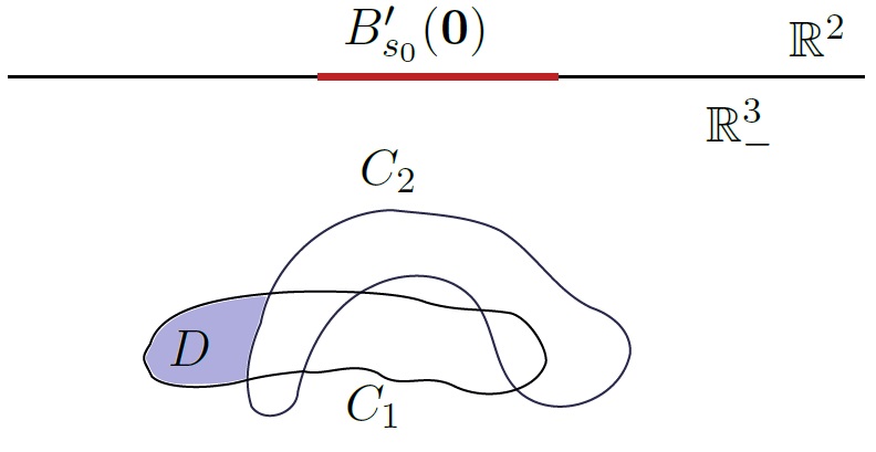
Figure 1: The two domains $C_{1}$ and $C_{2}$ and the domain $D$.

where the function $\bm{w_{2}}$ is well-defined and satisfies the elastostatic equations, finding

$$\int\limits_{D}\bigl{(}\mathbb{C}\widehat{\nabla}\bm{w}_{2}\bigr{)}:\widehat{\nabla}\bm{w}_{2}\,d\bm{x}=\int\limits_{\partial D}\bigl{(}\mathbb{C}\widehat{\nabla}\bm{w}_{2}\bm{n}\bigr{)}\cdot\bm{w}_{2}\,d\sigma(\bm{x}).$$

Since $\mathbb{C}\widehat{\nabla}\bm{w}_{2}\bm{n}=0$ on $\partial D\cap\partial C_{2}$ and by the unique continuation property $\mathbb{C}\widehat{\nabla}\bm{w}_{2}\bm{n}=\mathbb{C}\widehat{\nabla}\bm{w}_{1}\bm{n}$ on $\Gamma_{1}=(\partial D\cap\partial C_{1})\subset\partial G$, we get

$$\int\limits_{D}\bigl{(}\mathbb{C}\widehat{\nabla}\bm{w}_{2}\bigr{)}:\widehat{\nabla}\bm{w}_{2}\,d\bm{x}=\int\limits_{\Gamma_{1}}\bigl{(}\mathbb{C}\widehat{\nabla}\bm{w}_{1}\bm{n}\bigr{)}\cdot\bm{w}_{2}\,d\sigma(\bm{x})=0,$$

hence $\bm{w}_{2}=\mathbf{A}\bm{x}+\bm{a}$ in $D$, where $\mathbf{A}\in\mathbb{R}^{3\times 3}$ is a skew-symmetric matrix and $\bm{a}\in\mathbb{R}^{3}$. From the unique continuation principle applied to $\bm{w}_{2}-\mathbf{A}\bm{x}-\bm{a}$ we obtain that $\bm{w}_{2}=\mathbf{A}\bm{x}+\bm{a}$ in $\mathbb{R}^{3}_{-}\setminus\overline{C}_{2}$, hence $\bigl{(}\mathbb{C}\widehat{\nabla}\bm{w}_{2}\bigr{)}\bm{n}=0$ on $B^{\prime}_{s_{0}}(\bm{0})$, that is a contradiction.

The second case we analyse is related to the setting in Figure 2. To prove the contradiction, in this case we can consider, for example, the domain $D=D_{1}\cup D_{2}$, where $D_{1}$ and $D_{2}$ are represented in Figure 2.

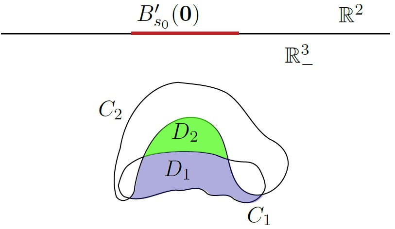
Figure 2: The two domains $C_{1}$ and $C_{2}$ and the domain $D=D_{1}\cup D_{2}$.

We emphasize that in this setting if we only consider the domain $D_{1}$ we will not be able to find a contradiction. In fact, from the unique continuation and the Green’s formula we would not be able to prove that the energy of the system related to the function $\bm{w}_{2}$ is equal to zero in $D_{1}$. Instead, considering the region $D$ and taking $\bm{w}_{2}$, which satisfies $\textrm{div}(\mathbb{C}\widehat{\nabla}\bm{w_{2}})=\bm{0}$ in $D$, from the Green’s formula we find, as before,

$$\int\limits_{D}\bigl{(}\mathbb{C}\widehat{\nabla}\bm{w}_{2}\bigr{)}:\widehat{\nabla}\bm{w}_{2}\,d\bm{x}=0,$$

hence $\bm{w}_{2}=\mathbf{A}\bm{x}+\bm{a}$ in $D$, with $\mathbf{A}\in\mathbb{R}^{3\times 3}$ a skew-symmetric matrix and $\bm{a}\in\mathbb{R}^{3}$. Applying the unique continuation principle to $\bm{w}_{2}-\mathbf{A}\bm{x}-\bm{a}$ we have that $\bm{w}_{2}=\mathbf{A}\bm{x}+\bm{a}$ in $\mathbb{R}^{3}_{-}\setminus\overline{C}_{2}$, hence $\bigl{(}\mathbb{C}\widehat{\nabla}\bm{w}_{2}\bigr{)}\bm{n}=0$ on $B^{\prime}_{s_{0}}(\bm{0})$, that is a contradiction. ∎

4.2 Stability Estimate

In this section we state and prove the stability estimates for our inverse problem by adapting the arguments contained in [15] and [16] to the case of a pressurized cavity in an unbounded domain. In order to keep the proof of the main result as readable as possible and since the strategy to get the stability theorem is similar of the one obtained in [15] we will not repeat all the details of the proofs of the auxiliary results we need. The main idea behind the stability result (Theorem 4.8) is to give a quantitative version of the uniqueness argument. More precisely, we combine two steps:

1. the propagation of the smallness of the Cauchy data up to the boundary of the cavities, leading to an integral estimate of the solutions (see Propositions 4.6 and 4.7);

2. an estimate of continuation from the interior (Proposition 4.4).

The basic tool for both steps is the three spheres inequality stated in Lemma 4.5.

In the sequel, for any $\varrho>0$, we denote by

$$\Omega_{\varrho}=\{\bm{x}\in\Omega\,:\,\textrm{dist}(\bm{x},\partial\Omega)>\varrho\}.$$

We first prove a regularity result on the solution of problem (4). To this end, we consider a bounded domain $Q\subset\mathbb{R}^{3}_{-}$ such that

$$\partial Q\in C^{3}\,\textrm{with constants}\,r_{0},E_{0},$$ (41)

$$\overline{B^{-}_{\alpha D_{0}}(\bm{0})}\subset\subset\overline{Q}\subset\subset\overline{B^{-}_{\beta D_{0}}(\bm{0})},$$ (42)

where $\alpha>2$ and $\beta\geq 3$, with $\alpha<\beta$. Now, we have the following regularity estimate.

Proposition 4.3.

Under the assumptions (35) for $C$ and (41), (42) for $Q$, the solution of problem (4), satisfies

$$\|\bm{u}\|_{C^{1,1/2}(\overline{Q}\setminus C)}\leq cp,$$ (43)

where the constant $c=c(\lambda,\mu,\alpha,\beta,r_{0},E_{0},D_{0})$.

Before proving this theorem, we briefly recall the integral representation formula for the solution to problem (4) derived in [7]. In particular, we define first the Neumann function, solution to

$$\begin{cases}\textrm{div}(\mathbb{C}\widehat{\nabla}{\mathbf{N}}(\cdot,\bm{y}))={\delta_{\bm{y}}}\mathbf{I}&\textrm{in }\,\mathbb{R}^{3}_{-}\\ (\mathbb{C}\widehat{\nabla}{\mathbf{N}}(\cdot,\bm{y}))\bm{n}=0&\textrm{on }\,\mathbb{R}^{2}\\ {\mathbf{N}}=O(|\bm{x}|^{-1}),\qquad|\nabla{\mathbf{N}}|=O(|\bm{x}|^{-2})&|\bm{x}|\to\infty,\end{cases}$$ (44)

where ${\delta_{\bm{y}}}$ is the delta function centred at $\bm{y}\in\mathbb{R}^{3}_{-}$ and $\mathbf{I}$ is the identity matrix (see Theorem A.1 in Appendix for its explicit expression). Then, for any $\bm{y}\in\overline{\mathbb{R}}^{3}_{-}\setminus\overline{C}$ we have

$$\bm{u}(\bm{y})=p\int\limits_{\partial C}\mathbf{N}(\bm{x},\bm{y})\bm{n}(\bm{x})\,d\sigma(\bm{x})-\int\limits_{\partial C}\big{[}\big{(}\mathbb{C}\widehat{\nabla}_{\bm{x}}\mathbf{N}(\bm{x},\bm{y})\big{)}\bm{n}(\bm{x})\big{]}^{T}\bm{f}(\bm{x})\,d\sigma(\bm{x}),$$ (45)

where $\bm{f}$ is the trace of $\bm{u}$ on $\partial C$ and $\bm{n}$ is the outer unit normal vector on $\partial C$ (for more details see [7]).

Proof of Theorem 4.3.

Since the kernels of the integral operators in (45) are regular for $\bm{y}\in\partial Q\setminus\partial C$, we can estimate $D^{k}\bm{u}(\bm{y})$, for $k=0,1,2,3$, getting easily

$$|D^{k}\bm{u}(\bm{y})|\leq p|\partial C|\,\sup\limits_{\mathclap{\begin{subarray}{c}\bm{x}\in\partial C\vspace{0.05cm}\\ \bm{y}\in\partial Q\setminus\partial C\end{subarray}}}|D^{k}_{\bm{y}}\mathbf{N}(\bm{x},\bm{y})|+|\partial C|^{1/2}\|\bm{f}\|_{L^{2}(\partial C)}\,\sup\limits_{\mathclap{\begin{subarray}{c}\bm{x}\in\partial C\vspace{0.05cm}\\ \bm{y}\in\partial Q\setminus\partial C\end{subarray}}}|D^{k}_{\bm{y}}(\mathbb{C}\widehat{\nabla}_{\bm{x}}\mathbf{N}(\bm{x},\bm{y}))|.$$

From the regularity properties of $\mathbf{N}$ and Theorem A.1 in Appendix, we have

$$\sup\limits_{\mathclap{\begin{subarray}{c}\bm{x}\in\partial C\vspace{0.05cm}\\ \bm{y}\in\partial Q\setminus\partial C\end{subarray}}}|D^{k}_{\bm{y}}\mathbf{N}(\bm{x},\bm{y})| \leq\frac{c}{D^{k+1}_{0}},\qquad\qquad\sup\limits_{\mathclap{\begin{subarray}{c}\bm{x}\in\partial C\vspace{0.05cm}\\ \bm{y}\in\partial Q\setminus\partial C\end{subarray}}}|D^{k}_{\bm{y}}(\mathbb{C}\widehat{\nabla}_{\bm{x}}\mathbf{N}(\bm{x},\bm{y}))| \leq\frac{c}{D^{k+2}_{0}},$$ (46)

where the constant $c=c(\lambda,\mu,\alpha)$. From the trace estimate applied in $Q$, we have

$$\|\bm{f}\|_{L^{2}(\partial C)}\leq c\|\bm{u}\|_{H^{1}_{w}(\mathbb{R}^{3}_{-}\setminus\overline{C})}\leq cp,$$ (47)

hence, from (46) and (47), we get

$$|D^{k}\bm{u}(\bm{y})|\leq cp,$$

where the constant $c=c(\lambda,\mu,\alpha,r_{0},E_{0},D_{0})$. Therefore

$$\|D^{k}\bm{u}\|_{L^{\infty}(\partial Q\setminus\partial C)}\leq cp,\qquad k=0,1,2,3.$$ (48)

Next, we apply the following global regularity estimate for the elastostatic system with Neumann boundary conditions (see [18], Theorem 6.6, p. 79) for $\bm{u}$ in $Q\setminus\overline{C}$, that is

$$\|\bm{u}\|_{H^{3}(Q\setminus\overline{C})}\leq c\bigg{(}\|\bm{u}\|_{L^{2}(Q\setminus\overline{C})}+\|(\mathbb{C}\widehat{\nabla}\bm{u})\bm{n}\|_{W^{3/2,2}(\partial(Q\setminus\overline{C}))}\bigg{)},$$ (49)

with $c=c(\lambda,\mu,\alpha,\beta,r_{0},E_{0},D_{0})$. Now, observe that by (34)

$$\|\bm{u}\|_{L^{2}(Q\setminus\overline{C})}\leq c\,\bigg{\|}\frac{\bm{u}}{\rho}\bigg{\|}_{L^{2}(\mathbb{R}^{3}_{-}\setminus\overline{C})}\leq cp,$$ (50)

where $c=c(\lambda,\mu,\alpha,\beta,r_{0},E_{0},D_{0})$, while, for the term $\|(\mathbb{C}\widehat{\nabla}\bm{u})\bm{n}\|_{W^{3/2,2}(\partial(Q\setminus\overline{C}))}$ we have

$$(\mathbb{C}\widehat{\nabla}\bm{u})\bm{n}=\bm{0},\quad\textrm{on}\,\partial Q\cap\{x_{3}=0\},\qquad\qquad(\mathbb{C}\widehat{\nabla}\bm{u})\bm{n}=p\bm{n},\quad\textrm{on}\,\partial C,$$

and since $\partial C$ is of class $C^{3}$ (see (35)) it follows $(\mathbb{C}\widehat{\nabla}\bm{u})\bm{n}\in C^{2}(\partial C)$, hence

$$\|(\mathbb{C}\widehat{\nabla}\bm{u})\bm{n}\|_{W^{3/2,2}(\partial C)}\leq cp.$$ (51)

Analogously, from the estimate (48) and the regularity of the boundary of $Q$, we find

$$\|(\mathbb{C}\widehat{\nabla}\bm{u})\bm{n}\|_{W^{3/2,2}(\partial Q\setminus\partial C)}\leq cp.$$ (52)

Therefore, collecting (50), (51) and (52), the estimate (49) gives

$$\|\bm{u}\|_{H^{3}(Q\setminus\overline{C})}\leq cp.$$

Finally, applying the Sobolev embedding theorem (43) follows. ∎

Proposition 4.4 (Lipschitz propagation of smallness).

Under the assumptions (5), (8), (9), (10) and (35), let $\bm{w}$ be the solution to (38). There exist $R\geq 3D_{0}$, $R=R(\lambda,\mu,r_{0},E_{0},D_{0})$, and $s>1$, $s=s(\lambda,\mu,E_{0})$, such that for every $\varrho>0$ and every $\overline{\bm{x}}\in(B^{-}_{R}(\bm{0})\setminus\overline{C})_{s\varrho}$, we have

$$\int\limits_{B_{\varrho}(\overline{\bm{x}})}|\widehat{\nabla}\bm{w}|^{2}\,d\bm{x}\geq\frac{c}{e^{a\varrho^{-b}}}\int\limits_{B^{-}_{R}(\bm{0})\setminus\overline{C}}|\widehat{\nabla}\bm{w}|^{2}\,d\bm{x},$$ (53)

where $a,b,c>0$ depend on $\lambda,\mu,r_{0},E_{0}$ and $D_{0}$.

The proof of this proposition is based on the application of the three-spheres inequality. For the reader’s convenience we recall here only the statement of the theorem in the case of the linear elasticity in a homogenous and isotropic medium; for a more general case and its proof one can refer to [2, 3].

Lemma 4.5 (Three spheres inequality).

Let $\Omega$ be a bounded domain in $\mathbb{R}^{3}$. Let $\bm{w}\in H^{1}(\Omega)$ be a solution to the Lamé system. There exists ${\vartheta^{*}}$, $0<{\vartheta^{*}}\leq 1$, only depending on $\lambda$ and $\mu$ such that for every $r_{1},r_{2},r_{3},\overline{r}$, $0<r_{1}<r_{2}<r_{3}\leq{\vartheta^{*}}\overline{r}$, and for every $\bm{x}\in\Omega_{\overline{r}}$ we have

$$\int\limits_{B_{r_{2}}(\bm{x})}|\widehat{\nabla}\bm{w}|^{2}\leq c\left(\displaystyle\int\limits_{B_{r_{1}}(\bm{x})}|\widehat{\nabla}\bm{w}|^{2}\right)^{\delta}\left(\displaystyle\int\limits_{B_{r_{3}}(\bm{x})}|\widehat{\nabla}\bm{w}|^{2}\right)^{1-\delta},$$ (54)

where $c>0$ and $\delta$, $0<\delta<1$, only depend on $\lambda$, $\mu$, $\frac{r_{2}}{r_{3}}$ and are monotone increasing functions of $\frac{r_{1}}{r_{3}}$.

Now, the Lipschitz propagation of smallness inequality can be proved.

Proof of Proposition 4.4.

Let us denote $\Omega=B^{-}_{R}(\bm{0})\setminus\overline{C}$, with $R\geq 3D_{0}$ to be chosen later. Since the hemisphere $B^{-}_{1}(\bm{0})$ has Lipschitz boundary with absolute constants $r^{*},E^{*}$, $B^{-}_{R}(\bm{0})$ has Lipschitz boundary with constants $r^{*}R,E^{*}$. Possibly worsening the regularity parameters of $C$, see (35), we can assume $E_{0}\geq E^{*}$ and $r_{0}\leq r^{*}R$, so that the boundary of $\Omega$ is of Lipschitz class with constants $r_{0}$ and $E_{0}$.

Following similar arguments as those in [15] with the simplification of mantaining as integrand function $|\widehat{\nabla}\bm{w}|^{2}$, we find that there exist $\varrho_{0}=\varrho_{0}(\lambda,\mu,r_{0},E_{0},R)$, with $0<\varrho_{0}<1$, and $s=s(\lambda,\mu,E_{0})$, $s>1$, such that for all $0<\varrho\leq\varrho_{0}$ and for all $\overline{\bm{x}}\in\Omega_{s\varrho}$, it holds

$$\int\limits_{B_{\varrho}(\overline{\bm{x}})}|\widehat{\nabla}\bm{w}|^{2}\,d\bm{x}\geq c_{1}\int\limits_{\Omega}|\widehat{\nabla}\bm{w}|^{2}\,d\bm{x}\left(\frac{c\varrho^{3}\displaystyle\int\limits_{\Omega_{(s+1)\varrho}}|\widehat{\nabla}\bm{w}|^{2}\,d\bm{x}}{\displaystyle\int\limits_{\Omega}|\widehat{\nabla}\bm{w}|^{2}\,d\bm{x}}\right)^{\sigma^{-A_{1}-B_{1}\log(1/\varrho)}},$$ (55)

where $c_{1}>0$ only depend on $\lambda,\mu$; $\sigma\in(0,1),s>1$ depend on $\lambda,\mu,E_{0}$ and $c,A_{1},B_{1}>0$ depend on $\lambda,\mu,E_{0},r_{0},R$. The main goal is to give a lower estimate of the ratio

$$\frac{\displaystyle\int\limits_{\Omega_{(s+1)\varrho}}|\widehat{\nabla}\bm{w}|^{2}\,d\bm{x}}{\displaystyle\int\limits_{\Omega}|\widehat{\nabla}\bm{w}|^{2}\,d\bm{x}}$$

to get the assertion of the theorem. To this end, we first notice that

$$\frac{\displaystyle\int\limits_{\Omega_{(s+1)\varrho}}|\widehat{\nabla}\bm{w}|^{2}\,d\bm{x}}{\displaystyle\int\limits_{\Omega}|\widehat{\nabla}\bm{w}|^{2}\,d\bm{x}}=1-\frac{\displaystyle\int\limits_{\Omega\setminus\Omega_{(s+1)\varrho}}|\widehat{\nabla}\bm{w}|^{2}\,d\bm{x}}{\displaystyle\int\limits_{\Omega}|\widehat{\nabla}\bm{w}|^{2}\,d\bm{x}}:=1-\frac{\mathcal{I}_{1}}{\mathcal{I}_{2}}.$$ (56)

Let us consider the integral $\mathcal{I}_{2}$. Since $\bm{w}=\bm{u}-\overline{\bm{u}}$, see (37), we use the integral representation formula $\eqref{representation formula}$ for the function $\bm{u}$ and the explicit expression of $\overline{\bm{u}}$ in (36). In detail, we consider

$$S=\bigg{\{}\bm{x}\in B^{-}_{R}(\bm{0})\,:\,x_{3}\leq-\frac{3}{4}R\bigg{\}}.$$ (57)

see Figure 3.

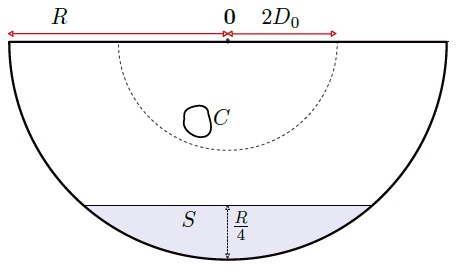
Figure 3: The region $S$.

By a simple calculation we have $|S|=(7/128)\pi R^{3}$.

If $\bm{x}\in\partial C$, $\bm{y}\in S$, then by (45) and Theorem A.1, it is easy to see that

$$|\widehat{\nabla}\bm{u}(\bm{y})|\leq|\nabla\bm{u}(\bm{y})|\leq\frac{cp}{R^{2}},\quad\forall\bm{y}\in S,$$

where $c=c(\lambda,\mu,r_{0},E_{0},D_{0})$, hence

$$|\widehat{\nabla}\bm{w}(\bm{y})|\geq|\widehat{\nabla}\overline{\bm{u}}(\bm{y})|-|\widehat{\nabla}\bm{u}(\bm{y})|\geq\frac{p}{3\lambda+2\mu}-\frac{cp}{R^{2}}\geq\frac{p}{2(3\lambda+2\mu)},$$

where the last inequality holds choosing $R=\max\{3D_{0},(2c^{-1}(3\lambda+2\mu))^{1/2}\}$. In this way, we have that

$$\mathcal{I}_{2}=\int\limits_{\Omega}|\widehat{\nabla}\bm{w}|^{2}\,d\bm{x}\geq\int\limits_{S}|\widehat{\nabla}\bm{w}|^{2}\,d\bm{x}\geq cp^{2}R^{3},$$ (58)

where $c=c(\lambda,\mu)$.

Now, we estimate the integral $\mathcal{I}_{1}$ using the regularity result of the Proposition 4.3. First, we split the integral domain as

$$\Omega\setminus\Omega_{(s+1)p}=F_{1}\cup F_{2},$$

where

$$F_{1}=\{\bm{x}\in\Omega\,:\,d(\bm{x},C))\leq(s+1)\varrho\},\qquad F_{2}=\{\bm{x}\in\Omega\,:\,d(\bm{x},\partial B^{-}_{R}(\bm{0}))\leq(s+1)\varrho\},$$

see Figure 4.

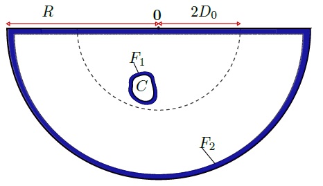
Figure 4: The region $\Omega\setminus\Omega_{(s+1)\varrho}$.

From (35), we notice that

$$|F_{1}\cup F_{2}|\leq c(r_{0},E_{0},D_{0})\varrho R^{2}.$$ (59)

Choosing in (42) $\alpha=R/D_{0}$, where $R=\max\{3D_{0},(2c^{-1}(3\lambda+2\mu))^{1/2}\}$, and $\beta=2\alpha$, then

$$\overline{B^{-}_{R}(\bm{0})}\subset\subset\overline{Q}\subset\subset\overline{B^{-}_{2R}(\bm{0})},$$

hence we apply the regularity estimate (43) for the two regions $F_{1}$ and $F_{2}$. Now, we have that

$$\|\widehat{\nabla}\bm{w}\|_{L^{\infty}(\Omega\setminus\Omega_{(s+1)\varrho})}\leq\big{(}\|\widehat{\nabla}\bm{u}\|_{L^{\infty}(\Omega\setminus\Omega_{(s+1)\varrho})}+\|\widehat{\nabla}\overline{\bm{u}}\|_{L^{\infty}(\Omega\setminus\Omega_{(s+1)\varrho})})\leq cp,$$

where $c=c(\lambda,\mu,r_{0},E_{0},D_{0})$. Therefore, from (59), we find

$$\mathcal{I}_{1}=\int\limits_{\Omega\setminus\Omega_{(s+1)\varrho}}|\widehat{\nabla}\bm{w}|^{2}\,d\bm{x}\leq cp^{2}\,|\Omega\setminus\Omega_{(s+1)\varrho}|\leq cp^{2}\varrho R^{2}.$$ (60)

Putting together inequalities (58) and (60), there exists $\varrho^{*}=\varrho^{*}(\lambda,\mu,r_{0},E_{0},D_{0})>0$, such that for any $\varrho\leq\varrho^{*}$, we have

$$\frac{\mathcal{I}_{1}}{\mathcal{I}_{2}}=\frac{\displaystyle\int\limits_{\Omega\setminus\Omega_{(s+1)\varrho}}|\widehat{\nabla}\bm{w}|^{2}\,d\bm{x}}{\displaystyle\int\limits_{\Omega}|\widehat{\nabla}\bm{w}|^{2}\,d\bm{x}}\leq\frac{1}{2}.$$

Going back to (55) and (56) we have

$$\int\limits_{B_{\varrho}(\overline{\bm{x}})}|\widehat{\nabla}\bm{w}|^{2}\,d\bm{x}\geq\bigg{(}c\varrho^{3}\bigg{)}^{\sigma^{-A_{1}-B_{1}\log(1/\varrho)}}\int\limits_{\Omega}|\widehat{\nabla}\bm{w}|^{2}\,d\bm{x},$$

where $c,A_{1},B_{1}$ depend on $\lambda,\mu,E_{0},r_{0},D_{0}$, for all $\varrho\leq\varrho^{*}$. To conclude, we take $\varrho\leq c$, hence, for every $\varrho\leq\min(c,\varrho^{*})$ and noticing that $\log\varrho\geq-1/\varrho$ for $0<\varrho<1$, we get the assertion choosing

$$a=6e^{A_{1}|\log\sigma|}\qquad\quad\textrm{and}\qquad\quad b=B_{1}|\log\sigma|+1.$$

∎

We omit the proof of the following two propositions, since they can be obtained using the same strategy adopted in proving Propositions 3.5 and 3.6 in [15].

Proposition 4.6 (Stability Estimates of Continuation from Cauchy Data).

Under the assumption (5) let $C_{1}$ and $C_{2}$ be two domains satisfying (8), (9), (10) and (35). Moreover, let $\bm{w}_{i}$, for $i=1,2$, be the solution to (38) with $C=C_{i}$. Then, for $\varepsilon<e^{-1}p$, we have

$$\int\limits_{C_{2}\setminus\overline{C}_{1}}|\widehat{\nabla}\bm{w}_{1}|^{2}\,d\bm{x}\leq cp^{2}\bigg{(}\log\Big{|}\log\frac{\varepsilon}{p}\Big{|}\bigg{)}^{-1/6},$$ (61)

$$\int\limits_{C_{1}\setminus\overline{C}_{2}}|\widehat{\nabla}\bm{w}_{2}|^{2}\,d\bm{x}\leq cp^{2}\bigg{(}\log\Big{|}\log\frac{\varepsilon}{p}\Big{|}\bigg{)}^{-1/6},$$

where the constant $c=c(\lambda,\mu,r_{0},E_{0},D_{0},s_{0})$.

The stability estimates in (61) can be improved when $\partial G$ is of Lipschitz class, where $G$ is defined by (40), as stated in the proposition below.

Proposition 4.7 (Improved Stability Estimates of Continuation from Cauchy Data).

Under the assumption (5) let $C_{1}$ and $C_{2}$ be two domains satisfying (8), (9), (10) and (35). In addition, let us assume that there exist $L>0$ and $\widetilde{r}_{0}$, with $0<\widetilde{r}_{0}\leq r_{0}$, such that $\partial G$ is of Lipschitz class with constants $\widetilde{r}_{0},L$. Then, we have

$$\int\limits_{C_{2}\setminus\overline{C}_{1}}|\widehat{\nabla}\bm{w}_{1}|^{2}\,d\bm{x}\leq cp^{2}\Big{|}\log\frac{\varepsilon}{p}\Big{|}^{-\gamma},$$ (62)

$$\int\limits_{C_{1}\setminus\overline{C}_{2}}|\widehat{\nabla}\bm{w}_{2}|^{2}\,d\bm{x}\leq cp^{2}\Big{|}\log\frac{\varepsilon}{p}\Big{|}^{-\gamma},$$

where $c,\gamma>0$ depend on $\lambda,\mu,r_{0},E_{0},D_{0},s_{0},L,\widetilde{r}_{0}$.

Now, we have all the preliminary results to prove the stability theorem.

Theorem 4.8 (Stability Estimate).

Under the assumption (5) let $C_{1}$ and $C_{2}$ be two domains satisfying (8), (9), (10) and (35). Moreover, let $\bm{u}_{i}$, for $i=1,2$, be the solution to (4) with $C=C_{i}$. If, given $\varepsilon>0$, we have

$$\|\bm{u}_{1}-\bm{u}_{2}\|_{L^{2}(B^{\prime}_{s_{0}}(\bm{0}))}\leq\varepsilon,$$ (63)

then it holds

$$d_{\mathcal{H}}(\partial C_{1},\partial C_{2})\leq c\bigg{(}\log\Big{|}\log\frac{\varepsilon}{p}\Big{|}\bigg{)}^{-\eta},$$ (64)

for every $\varepsilon<e^{-1}p$, where the constants $c$ and $\eta$, with $0<\eta\leq 1$, depend on $\lambda,\mu,r_{0},E_{0},D_{0}$ and $s_{0}$.

Proof.

Since (39) holds, we prove the assertion using the function $\bm{w}_{i}$, for $i=1,2$. In this way we can apply the same proof strategy contained in [16]. In the sequel we simply denote with $d_{\mathcal{H}}$ the Hausdorff distance $d_{\mathcal{H}}(\partial C_{1},\partial C_{2})$.

Let us prove that if $\eta>0$ is such that

$$\int\limits_{C_{2}\setminus\overline{C}_{1}}|\widehat{\nabla}\bm{w}_{1}|^{2}\,d\bm{x}\leq\eta,\quad\qquad\int\limits_{C_{1}\setminus\overline{C}_{2}}|\widehat{\nabla}\bm{w}_{2}|^{2}\,d\bm{x}\leq\eta,$$ (65)

then we have

$$d_{\mathcal{H}}\leq c\bigg{(}\log\frac{cp^{2}}{\eta}\bigg{)}^{-1/b},$$ (66)

where $b,c$ depend on $\lambda,\mu,r_{0},E_{0},D_{0}$.
We may assume, with no loss of generality, that there exists $\bm{x}_{0}\in\partial C_{1}$ such that

$$\textrm{dist}(\bm{x}_{0},\partial C_{2})=d_{\mathcal{H}}.$$

In this setting, we have to distinguish two cases:

1. $B_{d_{\mathcal{H}}}(\bm{x}_{0})\subset C_{2}$;

2. $B_{d_{\mathcal{H}}}(\bm{x}_{0})\cap C_{2}=\emptyset$.

Let us consider case (i). By the regularity assumption made on $\partial C_{1}$, see (35), there exists $\bm{x}_{1}\in C_{2}\setminus\overline{C}_{1}$ such that

$$B_{tdd_{\mathcal{H}}}(\bm{x}_{1})\subset(C_{2}\setminus\overline{C}_{1}),\,\textrm{with}\,\,\,t=\frac{1}{1+\sqrt{1+E^{2}_{0}}}.$$

By the first inequality in (65), taking $\varrho=tdd_{\mathcal{H}}/s$ in Proposition 4.4, we have

$$\eta\geq\int\limits_{C_{2}\setminus\overline{C}_{1}}|\widehat{\nabla}\bm{w}_{1}|^{2}\,d\bm{x}\geq\int\limits_{B_{\varrho}(\bm{x}_{1})}|\widehat{\nabla}\bm{w}_{1}|^{2}\,d\bm{x}\geq\frac{c}{e^{a\varrho^{-b}}}\int\limits_{B^{-}_{R}\setminus\overline{C}_{1}}|\widehat{\nabla}\bm{w}_{1}|^{2}\,d\bm{x},$$ (67)

where we recall that $R=R(\lambda,\mu,r_{0},E_{0},D_{0})$. By (58), we find that

$$\int\limits_{B^{-}_{R}\setminus\overline{C}_{1}}|\widehat{\nabla}\bm{w}_{1}|^{2}\,d\bm{x}\geq cp^{2},$$

so that, going back to (67), we have

$$\eta\geq\frac{cp^{2}}{\displaystyle e^{a\varrho^{-b}}}=\frac{cp^{2}}{\displaystyle e^{a(td_{\mathcal{H}}/s)^{-b}}}.$$ (68)

From this inequality it is straightforward to find (66).

Case (ii) can be proved in a similar way by substituting $\bm{w}_{1}$ with $\bm{w}_{2}$ in the previous calculations and employing the second inequality in (65).

Now, applying (61), that is taking

$$\eta=cp^{2}\bigg{(}\log\Big{|}\log\frac{\varepsilon}{p}\Big{|}\bigg{)}^{-1/6},$$

we obtain from (66) that

$$d_{\mathcal{H}}\leq c\bigg{(}\log\log\Big{|}\log\frac{\varepsilon}{p}\Big{|}\bigg{)}^{-1/b},$$ (69)

where we require $\varepsilon<e^{-e}p$ to have a positive quantity in right side of the previous inequality; the positive constants $b,c$ depend on $\lambda,\mu,r_{0},E_{0},s_{0}$ and $D_{0}$.

Next, to improve the modulus of continuity of this estimate we recall a geometrical result, first introduced and proved in [1], ensuring that there exists $d_{0}>0$, $d_{0}=d_{0}(r_{0},E_{0})$ such that if $d_{\mathcal{H}}(\partial C_{1},\partial C_{2})\leq d_{0}$, then the boundary of $G$ is of Lipschitz class with constants $\widetilde{r}_{0}$, $L$, only depending on $r_{0}$ and $E_{0}$. By (69), there exists $\varepsilon_{0}>0$ only depending on $\lambda,\mu,r_{0},E_{0},s_{0}$ and $D_{0}$ such that if $\varepsilon\leq\varepsilon_{0}$ then $d_{\mathcal{H}}\leq d_{0}$. In this way $G$ satisfies the hypotheses of Proposition 4.7 hence the assertion follows. ∎

Appendix A Neumann Function for the Lamé operator in the Half-Space

This appendix is devoted to the explicit expression of the Neumann function for the Lamé operator in the half-space presented in [13, 14]. Before doing that we recall the fundamental solution $\mathbf{\Gamma}$ of the Lamé operator, that is the so called Kelvin-Somigliana matrix. $\mathbf{\Gamma}$ is the solution to the equation

$$\textrm{div}(\mathbb{C}\widehat{\nabla}\bm{\Gamma})=\delta_{\bm{0}}\mathbf{I},\qquad\bm{x}\in\mathbb{R}^{3}\setminus\{\bm{0}\},$$

where $\delta_{\bm{0}}$ is the Dirac function centred at $\bm{0}$ and $\mathbf{I}$ is the identity matrix. Setting $C_{\mu,\nu}:={1}/\{16\pi\mu(1-\nu)\}$, where $\nu$ is the Poisson ratio $\nu=\lambda/(2(\lambda+\mu))$, the explicit expression of $\mathbf{\Gamma}=(\Gamma_{ij})$ is

$$\Gamma_{ij}(\bm{x})=-C_{\mu,\nu}\biggl{\{}\frac{(3-4\nu)\delta_{ij}}{|\bm{x}|}+\frac{x_{i}x_{j}}{|\bm{x}|^{3}}\biggr{\}},\qquad i,j=1,2,3,$$ (70)

where $\delta_{ij}$ is the Kronecker symbol.

Given $\bm{y}=(y_{1},y_{2},y_{3})$, we set $\widetilde{\bm{y}}=(y_{1},y_{2},-y_{3})$. Now, we have

Theorem A.1 ([7]).

The Neumann function $\mathbf{N}$ of problem (44) can be decomposed as

$$\mathbf{N}(\bm{x},\bm{y})=\mathbf{\Gamma}(\bm{x}-\bm{y})+\mathbf{R}^{1}(\bm{x}-\widetilde{\bm{y}})+y_{3}\mathbf{R}^{2}(\bm{x}-\widetilde{\bm{y}})+y_{3}^{2}\,\mathbf{R}^{3}(\bm{x}-\widetilde{\bm{y}}),$$

where $\mathbf{\Gamma}$ is the Kelvin matrix, see (70), and $\mathbf{R}^{k}$, $k=1,2,3$, have components $R^{k}_{ij}$ given by

$$R^{1}_{ij}(\bm{\eta}) :=C_{\mu,\nu}\bigl{\{}-(\tilde{f}+c_{\nu}\tilde{g})\delta_{ij}-(3-4\nu)\eta_{i}\eta_{j}\tilde{f}^{3}$$

$$\hskip 78.24507pt+c_{\nu}\bigl{[}\delta_{i3}\eta_{j}-\delta_{j3}(1-\delta_{i3})\eta_{i}\bigr{]}\tilde{f}\tilde{g}+c_{\nu}(1-\delta_{i3})(1-\delta_{j3})\eta_{i}\eta_{j}\tilde{f}\tilde{g}^{2}\bigr{\}}$$

$$R^{2}_{ij}(\bm{\eta}) :=2C_{\mu,\nu}\bigl{\{}(3-4\nu)\bigl{[}\delta_{i3}(1-\delta_{j3})\eta_{j}+\delta_{j3}(1-\delta_{i3})\eta_{i}\bigr{]}\tilde{f}^{3}-(1-2\delta_{3j})\delta_{ij}\eta_{3}\tilde{f}^{3}$$

$$\hskip 248.96161pt+3(1-2\delta_{3j})\eta_{i}\eta_{j}\eta_{3}\tilde{f}^{5}\bigr{\}}$$

$$R^{3}_{ij}(\bm{\eta}) :=2C_{\mu,\nu}(1-2\delta_{j3})\bigl{\{}\delta_{ij}\tilde{f}^{3}-3\eta_{i}\eta_{j}\tilde{f}^{5}\bigr{\}}.$$

for $i,j=1,2,3$, where $c_{\nu}:=4(1-\nu)(1-2\nu)$ and

$$\tilde{f}(\bm{\eta}):=\frac{1}{|\bm{\eta}|},\qquad\tilde{g}(\bm{\eta}):=\frac{1}{|\bm{\eta}|-\eta_{3}}.$$

References

References

- [1] Alessandrini G., Beretta E., Rosset E., Vessella S., Optimal stability for inverse elliptic boundary value problems with unknown boundaries. Ann. Scuola Norm. Sup. Pisa Cl. Sci. 4 (2000) 755–806.
- [2] Alessandrini G., Morassi A., Strong unique continuation for Lamé system of elasticity. Communications in Partial Differential Equations 26 (2001) 1787–1810.
- [3] Alessandrini G., Morassi A., Rosset E., Detecting an inclusion in an elastic body by boundary measurements. SIAM Journal of Mathematical Analysis 33 (2002) 1247–1268.
- [4] Alessandrini G., Morassi A., Rosset E., The linear constraints in Poincaré and Korn type inequalities. Forum Mathematicum 20 (2008) 557–569.
- [5] Amrouche C., Bonzom F., Exterior problems in the half-space for the Laplace operator in weighted Sobolev spaces. Journal of Differential Equations 246 (2009) 1894–1920.
- [6] Amrouche C., Dambrine M., Raudin Y., An theory of linear elasticity in the half-space. Journal of Differential Equations 253 (2012) 906–932.
- [7] Aspri A., Beretta E., Mascia C., Analysis of a Mogi-type model describing surface deformations induced by a magma chamber embedded in an elastic half-space. Journal de l’École Polytechnique — Mathématiques 4 (2017) 223–255.
- [8] Battaglia M., Hill D.P., Analytical modeling of gravity changes and crustal deformation at volcanoes: the Long Valley caldera, California, case study. Tectonophysics 471 (2009) 45–57.
- [9] Gurtin M.E., The Linear Theory of Elasticity, Encyclopedia of Physics, Vol VI a/2, Springer-Verlag, 1972.
- [10] Hanouzet B., Espaces de Sobolev avec poids. Application au problème de Dirichlet dans un demi-espace, Rend. Sem. Mat. Univ. Padova 46 (1971) 227–272.
- [11] Kondrat’ev V.A., Oleinik O.A., Boundary-value problems for the system of elasticity theory in unbounded domains. Korn’s inequalities. Russian Math. Surveys 43 (1988) 65–119.
- [12] Lisowski M., Analytical volcano deformation source models. in “Volcano Deformation. Geodetic Monitoring Techniques”, 279–304. Springer Praxis Books, editor: D.Dzurisin, 2006.
- [13] Mindlin R. D., Force at a Point in the Interior of a SemiInfinite Solid, Journal of Applied Physics 7 (1936) 195–202.
- [14] Mindlin R. D., Force at a Point in the Interior of a Semi-Infinite Solid, Proceedings of The First Midwestern Conference on Solid Mechanics, April, University of Illinois, Urbana, Ill. (1954).
- [15] Morassi A., Rosset E., Stable determination of cavities in elastic bodies. Inverse Problem 20 (2004) 453–480.
- [16] Morassi A., Rosset E., Uniqueness and stability in determining a rigid inclusion in an elastic body. Memoirs of the American Mathematical Society 200 volume 938 (2009) 453–480.
- [17] Segall P., Earthquake and volcano deformation. Princeton University Press, 2010.
- [18] Valent T., Boundary value problems of finite elasticity, local theorems on existence, uniqueness and analytic dependence on data. Springer-Verlag New York Berlin Heidelberg, 1988.
- [19] Weck N., Außenraumaufgaben in der Theorie stationärer Schwingungen inhomogener elasticher Körper. Math. Z. 111 (1969) 387-398.