Towards the exact Bremsstrahlung function of ABJM theory
Abstract
We present the three-loop calculation of the Bremsstrahlung function associated to the 1/2–BPS cusp in ABJM theory, including color subleading corrections. Using the BPS condition we reduce the computation to that of a cusp with vanishing angle. We work within the framework of heavy quark effective theory (HQET) that further simplifies the analytic evaluation of the relevant cusp anomalous dimension in the near–BPS limit. The result passes nontrivial tests, such as exponentiation, and is in agreement with the conjecture made in Bianchi:2014laa for the exact expression of the Bremsstrahlung function, based on the relation with fermionic latitude Wilson loops.
Keywords:
ABJM theory, BPS Wilson loops, Cusp anomalous dimension, Bremsstrahlung function1 Introduction
Wilson loops (WLs) play an ubiquitous role in gauge theories, both at perturbative and non–perturbative level. Depending on the particular contour, they encode the potential between heavy colored sources and control important aspects of scattering between charged particles. At the same time they provide the basis for the lattice formulation of any gauge theory and represent a general class of observables with deep mathematical meaning. The AdS/CFT correspondence Maldacena:1997re ; Witten:1998qj ; Gubser:1998bc has triggered further interest for WLs in supersymmetric gauge theories. In fact, they are directly related to fundamental string or brane configurations of the dual theory and are natural observables capable of testing the correspondence itself Maldacena:1998im ; Rey:1998ik . For example, the vacuum expectation values of some BPS WLs are non–trivial functions of the gauge coupling, potentially providing an interpolation between weak and strong coupling regimes. The exact computation of these quantities is sometimes possible, for instance using localization techniques Pestun:2007rz ; Kapustin:2009kz , offering non–trivial tests of the AdS/CFT predictions Erickson:2000af ; Drukker:2000rr .
When the theory is conformal, WLs govern the computation of the energy radiated by a moving quark in the low energy limit, the so–called Bremsstrahlung function Correa:2012at . This function also enters the small angle expansion of the cusp anomalous dimension that, in turn, controls the short distance divergences of a WL in the proximity of a cusp, according to the universal behaviour (where and are IR and UV cutoffs, respectively). Precisely, for supersymmetric WLs given as the holonomy of generalized connections that include also couplings to matter, we can consider a cusped WL depending on two parameters, representing the geometric angle between the two Wilson lines defining the cusp, and the latitude angle describing the change in the orientation of the couplings to matter between the two rays Drukker:1999zq ; Drukker:2011za . At the cusped WL is BPS, therefore finite, and its anomalous dimension vanishes. For small angles, , the expansion of around the BPS point reads
| (1.1) |
where is the Bremsstrahlung function, given as a function of the coupling constant of the theory.
In SYM theory an exact prescription to extract this non–BPS observable from BPS loops has been given in the seminal paper Correa:2012at , where results from localization where explicitly used. The very same result can be obtained by starting from an exact set of TBA equations Bombardelli:2009ns ; Gromov:2009bc ; Arutyunov:2009ur describing the generalized cusp Correa:2012hh ; Drukker:2012de , solving the system in the near–BPS limit Gromov:2012eu . Actually, using integrability, one can further obtain a Bremsstrahlung function , by considering the insertion of some chiral operator of R–charge L on the tip of the cusp Gromov:2013qga . This last result still calls for a localization explanation (see some progress in this direction in Bonini:2015fng ). Moreover, the use of the quantum spectral curve techniques Gromov:2013pga ; Gromov:2014caa has allowed to obtain results away from the BPS point Gromov:2015dfa . A proposal for the Bremsstrahlung function in four dimensional SYM appeared more recently in Fiol:2015spa .
It is quite natural to extend the above investigations to the three–dimensional case, exploring the Bremsstrahlung function in superconformal ABJ(M) theories Aharony:2008ug ; Aharony:2008gk . One immediately faces a first difference with the four-dimensional case: In ABJ(M) models not only bosonic but also fermionic matter can be used to build up generalized (super)connections whose holonomy gives rise to supersymmetric loop operators. Precisely, there are two prototypes of supersymmetric Wilson lines, one associated to a generalized gauge connection that includes couplings to bosonic matter only, so preserving 1/6 of the original supersymmetries Berenstein:2008dc ; Drukker:2008zx ; Chen:2008bp ; Rey:2008bh , and another one in which the addition of local couplings to the fermions enhances the operator to be 1/2–BPS Drukker:2009hy . The latter should be dual to the fundamental string on . While the 1/2 BPS operator is cohomologically equivalent (and therefore basically indistinguishable) to a linear combination of 1/6 BPS ones, the fact that they preserve different portions of supersymmetry allows for constructing different non–BPS observables starting from them. Generalized cusps formed with 1/6-BPS rays or 1/2-BPS rays are actually different Griguolo:2012iq ; Lewkowycz:2013laa and, consequently, different Bremsstrahlung functions can be defined and potentially evaluated exactly. In particular, in Lewkowycz:2013laa a proposal for the exact Bremsstrahlung function of the 1/6-BPS cusp was put forward, based on the localization result for the 1/6-BPS circular WL, and an extension to the 1/2-BPS case was conjectured.
In Bianchi:2014laa an exact formula appeared that expresses the Bremsstrahlung function for 1/2–BPS quark configurations as the derivative of a fermionic latitude WL with respect to the latitude angle. This proposal was suggested by the analogy with the SYM case Correa:2012at and supported by an explicit two–loop computation that agrees with the result obtained directly from the cusp with 1/2–BPS rays Griguolo:2012iq . Given that the fermionic latitude WL is cohomologically equivalent to a bosonic latitude WL Bianchi:2014laa , can be eventually expressed as
| (1.2) |
in terms of the well–known vev of 1/6-BPS WLs associated to the two gauge groups and computed exactly at framing one using localization Kapustin:2009kz ; Marino:2009jd ; Drukker:2010nc . Remarkably, this formula coincides with the proposal of Lewkowycz:2013laa , despite being derived from different arguments. Such an expression is also in agreement with a one-loop string computation at strong coupling Forini:2012bb ; Aguilera-Damia:2014bqa ; Correa:2014aga .
Expanding the matrix model result for and at weak coupling one can infer that in the planar limit this expression contains odd powers of the ’t Hooft coupling only. In principle, there should be a second contribution to (1.2) proportional to the derivative of a multiply –wound 1/6–BPS circular WL with respect to . This term should provide the even power expansion in . However, using the exact expression for the –wound WL known from localization, we can verify that both at weak and strong coupling this term vanishes (at least) in the planar limit Lewkowycz:2013laa ; Bianchi:2014laa . In particular, up to two loops it vanishes also at finite .
Based on this observation and using the weak coupling expansion of and as derived from the matrix model (including the color subleading contributions), eq. (1.2) gives the following prediction for the function, at any finite
| (1.3) |
The first term has been already checked in Bianchi:2014laa . In order to put this conjecture on more solid bases, further checks at higher orders are desirable. In this paper we perform a three–loop computation of directly from its definition in term of the fermionic cusped WL. As a result we obtain exactly the predicted coefficient in (1.3), so providing a highly non–trivial test of the proposal Bianchi:2014laa ; Lewkowycz:2013laa . In particular, at least up to three loops, we have checked that (1.2) is valid not only in the planar limit, but also at finite . We remark that since we are checking the Bremsstrahlung function through an odd perturbative order, our test is independent of any assumption on the even– part that was discarded in (1.2), according to the discussion above.
To simplify the three–loop calculation, we rely on the BPS condition satisfied by the fermionic cusped WL Griguolo:2012iq that implies the small angle expansion (1.1). From this equation we can read the Bremsstrahlung function equivalently from the or the expansions of , setting the other angle to zero. It turns out to be particularly convenient to set (flat cusp limit), working with the internal angle only. As will be discussed in details, this choice leads to crucial simplifications at several stages of the calculation.
As usual, when computing the cusped WL in the near–BPS limit UV and IR divergences arise. Here we employ dimensional regularization with dimensional reduction (DRED) to regulate the UV divergences and introduce an IR suppression factor to tame the IR divergences coming from the integration region at large distances. The cusp anomalous dimension is then obtained through the usual renormalization group equation for the renormalized cusped WL Korchemsky:1987wg . The calculation is carried out in momentum space where the Wilson lines are effectively described by non–relativistic, eikonal propagators. This procedure has a physical interpretation in the context of heavy quark effective theory (HQET) Gervais:1979fv ; Dotsenko:1979wb ; Arefeva:1980zd .
The plan of the paper is the following. In section 2 we review the construction of 1/2–BPS WLs in ABJM theories and present the proposal for the exact 1/2–BPS Bremsstrahlung function, as derived in Bianchi:2014laa . In section 3 we outline the strategy of the three–loop computation, describing in particular the HQET formalism. Section 4 contains a review of the one– and two–loop results that are important in order to check the correct exponentiation. The actual three–loop calculation appears in section 5, while the Bremsstrahlung function is extracted in section 6. Section 7 contains our conclusions. Many technical details, together with the results for the relevant two– and three–loop diagrams are deferred to eight appendices.
2 Exact 1/2–BPS Bremsstrahlung in ABJM theory
2.1 The 1/2–BPS cusp in ABJM
We start reviewing the definition of the locally 1/2–BPS cusp in ABJM theory 111Generalities on the ABJM theory in our conventions are given in appendices B, C.. This is constructed by considering the fermionic WL 222 Here the path–exponential is defined by
| (2.1) |
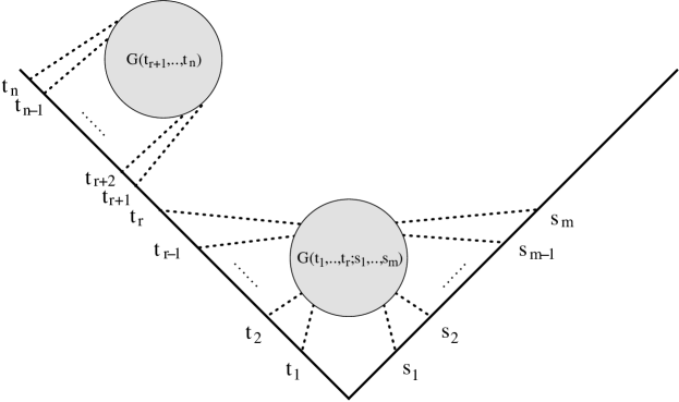
evaluated along the contour formed by two rays lying in the plane and intersecting at the origin, as illustrated in figure 1.
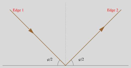
The angle between the rays is , such that for they form a continuous straight line. Explicitly, the contour drawn in figure 1 is parametrized as
| (2.2) |
In (2.1) is a superconnection belonging to the Lie-superalgebra and given by
| (2.3) |
Here denotes the standard matrix trace (and not the super–trace, see Griguolo:2012iq for a detailed discussion). The fermionic couplings on each straight–line possess the factorized structure Drukker:2009hy ; Griguolo:2012iq
| (2.4) |
The lowercase index distinguishes the two different rays forming the cusp. On the first edge, the spinor and R–symmetry factors are respectively given by
| (2.5) |
while on the second one we have
| (2.6) |
The angle is the counterpart of in the R–symmetry space. It denotes the angular separation of the two edges in the internal space (i.e. ). The two matrices which couple the scalars are determined in terms of the vectors and through the relations . We have respectively
| (2.7) |
As discussed in details in Griguolo:2012iq the presence of two angles allows us to find BPS configurations. Explicitly, for the two straight lines forming the cusp share two Poincarè supercharges and two conformal supercharges. In other words we deal with a globally BPS WL. As a consequence, the divergent contributions arising from the cusp geometry are expected to vanish if the BPS condition is satisfied, a fact which was explicitly checked up to second order in perturbation theory Griguolo:2012iq .
2.2 The exact 1/2–BPS Bremsstrahlung function
Away from the BPS point , the cusped WL defined above suffers in general from UV divergences. At generic angles it has to be renormalized and we expect that the operator possesses an anomalous dimension , according to the universal behaviour
| (2.8) |
where is an IR cutoff and stems for the renormalization scale. For the familiar bosonic WL, the divergences associated to a cusp singularity along the contour can be cast in the exponential form (2.8) Korchemsky:1987wg . This property follows from the presence of general exponentiation theorems for these operators. More precisely, their expectation value can be written as the exponential of the sum of all two–particle irreducible diagrams Dotsenko:1979wb ; Gatheral:1983cz . Extending these results to our case is not straightforward. In fact, the additional couplings between the contour and the fermions appearing in the superconnection may affect the standard analysis presented there. However, despite of these potential technical issues, we expect the trace of the Wilson line in ABJM to respect the usual exponentiation process, so that we can define an anomalous dimension for the cusp according to the standard text–book procedure. Our three–loop result will explicitly confirm the consistency of this picture (see discussion in section 6).
In the limit where the cusp angle is small, the cusp anomalous dimension has a Taylor expansion in even powers of , whose first coefficient is defined as the Bremsstrahlung function Correa:2012at . The 1/2–BPS cusp , associated to the 1/2–BPS Wilson lines (2.1) of the ABJM theory, vanishes for and consequently the small angle expansion reads
| (2.9) |
where is a function of the coupling and the number of colors only.
In Bianchi:2014laa a conjecture was put forward for the exact expression of . The argument was articulated in a few steps, which we briefly review here.
-
•
First, the Bremsstrahlung function was related to the expectation value of a supersymmetric fermionic circular WL evaluated on latitude contours in the sphere, that is displaced by an angle from the maximal circle, and potentially by an additional internal angle in the R–symmetry space. Remarkably, the expectation value of such WL seems to depend only on a particular combination of the angles, Bianchi:2014laa . The undeformed contour yields the 1/2–BPS circular WL of Drukker:2009hy and corresponds to .
Paralleling an analogous derivation for SYM Correa:2012at , the conjecture of Bianchi:2014laa states that the Bremsstrahlung function is retrieved by taking derivatives of the WL expectation value with respect to the characteristic parameter measuring the deformation
(2.10) Unfortunately, in contrast with the SYM case, the latitude WLs have not been yet evaluated via localization, so more work is necessary to derive an exact formula for the Bremsstrahlung function.
-
•
As a second step, the expectation value of the latitude WL was argued to be expressible, via a cohomological equivalence, in terms of bosonic WL operators and preserving lower supersymmetry. Using this equivalence, eq. (2.10) can then be rewritten as
(2.11) where stands for the phase of the WL . Again, in the limit, such WL operators land on the 1/6–BPS circular WL of Chen:2008bp ; Rey:2008bh ; Drukker:2008zx and the cohomological equivalence parallels that for 1/2–BPS operators, described in Drukker:2009hy .
-
•
The expectation value of operators is not known exactly, either. Nevertheless, it was conjectured that at least the relevant derivative in (2.11) could be traded with the derivative of the expectation value of a multiply wound 1/6–BPS circular WL with respect to the winding number , upon proper identification of the latitude and winding parameters
(2.12) Such a trick was also proposed in Lewkowycz:2013laa in the case of the Bremsstrahlung function associated to a cusp constructed with two locally 1/6–BPS rays in ABJM theory. Multiply wound supersymmetric WLs were explored in details in Klemm:2012ii , where their expectation value was given using a matrix model average description.
-
•
The expansion of the results for and provides evidence that (2.12) vanishes at all orders, as advocated in Lewkowycz:2013laa ; Bianchi:2014laa , at least in the planar limit. Under these circumstances, we then arrive at the following simple proposal for the 1/2–BPS Bremsstrahlung function at all orders 333The subscript 1 indicates that the computation is performed at framing 1.
(2.13) The Bremsstrahlung function associated to a 1/2–BPS cusped WL is given in terms of the expectation value of the 1/6–BPS circular WL, well–known from localization Kapustin:2009kz ; Drukker:2010nc . In Griguolo:2012iq it has been checked that at two loops (2.12) vanishes also for finite . Therefore, up to three loops expression (1.3) provides the expected result for , without requiring the planar limit. This is the prediction that we are going to check with an explicit three–loop calculation of .
Somewhat unusually in ABJM theory, such an object seems to possess an odd dependence on the coupling . Nevertheless, the proposal is in agreement with previously derived results for the cusp anomalous dimension at weak coupling Griguolo:2012iq , that is up to two–loop order and up to subleading order at strong coupling Forini:2012bb ; Aguilera-Damia:2014bqa ; Correa:2014aga . In this paper we put the conjecture on much firmer grounds, by providing an explicit check of it up to three loop order in perturbation theory, including the sub-leading corrections in , which first appear at this order.
3 Overview of the computation
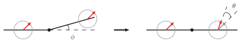
Referring to eq. (2.9), the Bremsstrahlung function can be read equivalently from the or the expansions, setting the other angle to 0
| (3.1) |
We take advantage of this fact for simplifying the evaluation of the Bremsstrahlung function, circumventing the computation of the complete cusp anomalous dimension. In particular, it proves convenient to set and work with the internal angle only, as shown in the cartoon of figure 2. This strategy brings dramatic simplifications at several stages of the computation, both in the number of diagrams to be taken into account and in their evaluation.
3.1 The diagrams
We now discuss how to suitably choose the computational setting in order to pin down the calculation to a relatively small number of Feynman diagrams to be considered at three loops.
First of all, we recall that in Chern–Simons–matter theories remarkable simplifications arise when the WL contour lies in a two–dimensional plane. In fact, this choice triggers the vanishing of several tensor contractions, by virtue of the antisymmetric nature of Chern–Simons gauge propagators (• ‣ C) and cubic vertex (C.5) in their index structure. In particular, whenever an odd number of antisymmetric tensors arises in the algebra of a diagram, their product eventually vanishes. In fact, one can always reduce them to a single Levi–Civita tensor whose indices have to be contracted with three external vectors. The latter all come from the WL contour and hence, lying on a plane, are not linearly independent and always give vanishing expressions when contracted with the tensor.
This feature of perturbation theory becomes particularly powerful at odd loop orders. Namely, from ABJM Feynman rules (see appendix C), one can infer that purely bosonic diagrams with gauge interactions vanish identically, by virtue of the aforementioned mechanism. For supersymmetric WLs this singles out contributions containing matter exchanges only. Nonetheless, there are still a number of simplifications.
For example, bosonic 1/6–BPS WL diagrams with scalar exchanges also evaluate to zero, thanks to the vanishing of the trace of their coupling matrices . Therefore, in ABJM theory bosonic WLs with planar contours, when computed at framing zero, automatically have vanishing expectation values at odd loops Rey:2008bh 444 A three–loop calculation at non–zero framing leads instead to a non–vanishing result Bianchi:2016yzj that matches the matrix model prediction..
As a consequence, only fermionic WLs of the Drukker–Trancanelli type Drukker:2009hy allow for nontrivial contributions at odd orders, as shown in Bianchi:2016vvm . This is precisely the class of WLs we are computing in this paper.
The arguments provided above imply that in our computation we have to consider only graphs containing at least one matter propagator. This condition substantially narrows down the number of diagrams to be considered.
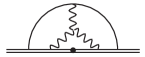
A further simplification arises from performing the calculation at , as previously discussed. In fact, taking the contour to lie on a straight line triggers the additional vanishing of diagrams such as the one in figure 3, again by antisymmetry in the contraction of tensors with vectors on the line.
Finally, aimed at computing the Bremsstrahlung function, one could in principle restrict to diagrams producing factors of only (see eq. (3.1)). According to the rules in appendix E, these occur only if a fermion line or a scalar bubble stretch between opposite sides of the cusp. Nevertheless, it turns out that we can easily compute the whole cusp at including also independent terms.
Technically, evaluating the various diagrams entails a few steps. After using the Feynman rules reviewed in appendix C, the integral associated to a generic diagram with fermion exchanges has the following structure
| (3.2) |
where and we have used the shortening notation . The number of internal and contour integrations, spinor structures, derivatives and propagators depend on the particular diagram. Lorentz indices carried by velocities, gamma matrices and derivatives are contracted among themselves or with external tensors. If couplings with scalars are also present, –matrix structures will appear.
We use identities in appendix E to reduce the bilinears and the –matrix structures. We perform the relevant tensor algebra strictly in three dimensions and in an automated manner with a computer program. In this process we drop all the terms containing an odd number of Levi–Civita tensors and reduce all the products of an even number of them to products of metric tensors. We finally arrive at expressions containing scalar products of velocities and derivatives only, where the ultimate step consists in integrating over internal vertices and WL parameters.
3.2 The integrals and the HQET formalism
The most striking simplification of working at is that the integrals arising from Feynman graphs reduce to propagator–type contributions which evaluate to numbers rather than functions of the angle, considerably reducing the effort needed for their determination.
The integrals could in principle be evaluated directly by solving internal integrations in configuration space and then integrating over the Wilson line parameters. In this case one could make use of the Gegenbauer polynomial –space technique GPXT Chetyrkin:1980pr to solve the three–dimensional internal integrals along the lines of Mauri:2013vd . However this approach becomes cumbersome and impractical for contributions with more than one internal integration, such as those appearing at three loops.
A more powerful strategy consists in Fourier transforming the integrals to momentum space and perform the contour integrations first. This step casts the various contributions into the form of the non–relativistic Feynman integrals appearing in the effective theory of heavy quarks (HQET) (see Grozin:2014hna ; Grozin:2015kna , for a recent application in four dimensions), or rather an Euclidean version thereof, as we perform the whole computation with signature.
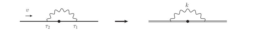
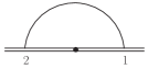
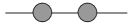
This procedure, applied to a single propagator, is sketched pictorially in figure 4. A more detailed application is described in sections 4 and 5.2, when dealing with the example of the one–loop and a particular graph of the three–loop computation. The velocity of the heavy quark is the vector tangent to the WL contour, .
In general, the resulting integrals suffer from both IR and UV divergences. UV divergences are treated within the framework of dimensional regularization, shifting spacetime integrations to dimensions. As a consequence, the integrals evaluate to Laurent series in the regularization parameter . In order to preserve supersymmetry we work in the dimensional reduction scheme (DRED) Siegel:1979wq . In practice this translates in performing the tensor algebra in the numerators strictly in three dimensions. This prescription can introduce evanescent terms if some tensor integration is attained (in ) and then contractions with three dimensional objects are carried out. Such evanescent terms can be taken into account by suitable regulator dependent factors (see e.g. Bianchi:2013rma ; Griguolo:2013sma ; Bianchi:2013pva for a discussion in the context of WLs in three dimensions). However, in the present case this subtlety is already built–in in our method and does not cause any practical worry. In fact, the index algebra is always handled (in integer dimensions) before any integration, as recalled in the previous section. After this reduction, the only potentially dangerous integrals occur whenever a tensor numerator contains contractions with an tensor, but such contributions were argued to vanish and promptly discarded.
In order to tame IR divergences at long distances along the WL contour, following Grozin:2015kna we introduce an exponential damping factor () for each contour integral, enforcing the finiteness of the integrals at large radius. This introduces a residual energy in the heavy quark, shifting the HQET propagators by
| (3.3) |
The parameter is customarily set to , a choice which simplifies the result of the relevant integrals. The final result for the cusp anomalous dimension is scheme independent and is not affected by the particular value of , albeit all intermediate steps might be.
Up to three loops, HQET propagator integrals were studied in detail in Grozin:2000jv ; Chetyrkin:2003vi for QCD in four dimensions. The analysis performed there reveals that all topologies can be reduced to a set of 1, 2 and 8 master integrals (seven planar and one non–planar) at one, two and three loop order, respectively, by means of integration by parts identities Tkachov:1981wb ; Chetyrkin:1981qh . Such a statement is true, independently of the space–time dimensions and applies to our case as well. This reduction step can be made automatic thanks to the Laporta algorithm Laporta:1996mq ; Laporta:2001dd and carried out with one of its available implementations Smirnov:2008iw ; Smirnov:2013dia ; Smirnov:2014hma ; Lee:2012cn ; Lee:2013mka . In practice we have used FIRE5 Smirnov:2014hma , whose C++ version is able to perform the reduction of all the required integrals in a few minutes on a PC.
The relevant master integrals have to be evaluated in dimensions. This task can be carried out straightforwardly relying on previously derived results for such topologies with general integration dimension and powers of the propagators Grozin:2000jv (some of them are non–integer because arising from the integration of bubble sub–topologies). The final evaluation of the master integrals and expansion in series of up to the desired order for the cusp anomalous dimension is spelled out in appendix F.
The procedure described above that reduces the cusp loop integrals to propagator–type integrals for non–relativistic heavy particles, has a very suggestive physical interpretation. The anomalous dimension of the cusped WL captures the renormalization of the current associated to a massive quark, undergoing a transition from a velocity to a velocity at an angle . In fact Wilson lines have been thoroughly employed as a convenient tool for describing the dynamics of such objects. According to this physical picture, the 1/2–BPS Wilson line in ABJM theory is associated to heavy quarks, which are interpreted as supermultiplet bosons, transforming in the fundamental representations of the two gauge groups. These were shown to arise when moving away from the origin of the moduli space Lee:2010hk ; Lietti:2017gtc .
The Bremsstrahlung function controls the energy loss by radiation of these massive particles undergoing a deviation by an infinitesimal angle. In particular, the Higgsing procedure mentioned above reveals that this superparticle is able to radiate off pairs of bifundamental fields, both scalars and fermions, quite exotically. The coupling to such matter fields enters the superconnection (2.3) of the 1/2–BPS Wilson line via a parameter , which can be interpreted as an angle in the internal R–symmetry space. According to the discussion above, we determine the Bremsstrahlung function by considering the equivalent (but computationally simpler) picture of a heavy quark subject to a small kick in R–symmetry space at fixed vanishing geometrical angle.
In particular, thanks to the condition, the integrals involved in the computation of the Bremsstrahlung function are precisely those contributing to the self–energy corrections of a heavy quark, i.e. propagator–type. The presence of the cusp point on the line has the simple effect of increasing the power of a HQET propagator in the diagram. Integration by parts identities can then be employed to reduce the power of the doubled propagator to unity.
3.3 The cusp anomalous dimension at zero angle
In the previous subsection we explained how the computation of the expectation value of the cusped WL is performed up to three loops, in the flat cusp limit. In this section we provide the details on how the cusp anomalous dimension and the Bremsstrahlung function can be practically extracted from this result.
As recalled above, the expectation value of the cusped WL suffers from UV and IR divergences. The former determine the renormalization properties of the WL and are the crucial object of our investigation. The latter can be regulated in different ways, either by assigning the heavy quarks a residual energy offsetting them from the mass shell as described above or by computing the loop on a finite interval as done in Griguolo:2012iq . Although these divergences are uninteresting for our purposes, different kinds of regularizations can be more or less convenient according to the approach we use to compute the integrals. Therefore, while discussing how to extract the UV divergent behavior of the cusped WL, we will also compare the effectiveness of different IR regularization strategies.
For a cusped WL in a gauge theory UV divergences may have different origins. The first source consists in the divergences of the Lagrangian. In particular, this can cause a running coupling and the presence of a nontrivial function. The ABJM model is superconformal and such a phenomenon does not occur. Then, divergences associated to the short distance behavior of the Wilson line can arise. In the language of HQET these are the (potentially divergent) radiative corrections to the self–energy of the heavy quarks. Finally, the cusp geometry itself introduces further divergent contributions, which are the ones we are interested in.
The systematics of the renormalization properties of WLs with cusps were discussed in Dorn:1986dt ; Korchemsky:1987wg . Here we recall some basic and general features.
First of all we can focus our attention only on contributions which are 1PI vertex diagrams in HQET language. For instance if we deal with a configuration of the type represented in figure 5 the subsector governed by the Green function completely decouples from the rest. In fact the corresponding contribution is factorized as
| (3.4) |
If we perform the change of variables and we use that is a translationally invariant function we find
| (3.5) |
The factor in (3.5) provides the value of the diagram obtained from the one in figure 5 removing the subsector governed by , while the factor is the contribution due to to the vacuum expectation value of a straight-line running from to . In HQET language this factorization is a trivial manifestation of momentum conservation. On the other hand, we have to stress that eq. (3.5) also relies on the judicious choice of the IR regulator which breaks translation invariance along the two rays of the cusp in a controlled way. For instance, if we were to tame the IR divergences by considering a cusp with edges of finite length , it is easy to see that the above argument would fail and the two contributions would remain in general intertwined.
Because of (3.5) the cusped WL is given by the sum of all the 1PI diagrams, which we shall denote by , times the vacuum expectation value of the Wilson lines , running from to and from to
| (3.6) |
The two Wilson line factors in HQET language are identified with the two point functions of the heavy quark and eq. (3.6) is the usual and well–known decomposition of the vacuum expectation value in terms of its 1PI sector and two-point functions.
To single out the cusp anomalous dimension from , we have first to eliminate the spurious divergences which are due to the fact that the presence of the IR regulator mildly breaks gauge invariance 555The integral of a total derivative along of the whole contour is no longer zero because of the presence of this factor.. A similar phenomenon also occurs when we consider edges of finite length Craigie:1980qs ; Aoyama:1981ev ; Knauss:1984rx ; Dorn:1986dt : There the gauge invariance is lost because the loop is open. In both cases the gauge–dependent divergent terms can be eliminated by introducing a multiplicative renormalization Craigie:1980qs ; Aoyama:1981ev ; Knauss:1984rx ; Dorn:1986dt , which, in practice, is equivalent to the subtraction of the straight line or the cusp at
| (3.7) |
with defined in (3.6). In the formalism of Gervais:1979fv corresponds to the wave-function renormalization of the fermions in the one-dimensional effective description of the Wilson line operator. This factor needs to be eliminated in order to single out the proper renormalization of the relevant operator describing the cusp Korchemsky:1987wg .
Finally we can extract by defining the renormalized WL as follows
| (3.8) |
The cusp anomalous dimension is then evaluated through the relation
| (3.9) |
where stems for the renormalization scale and we have suppressed the dependence on the angles.
The perturbative computation yields as an expansion in
| (3.10) |
In dimensional regularization every coefficient is given by a Laurent expansion in . According to the standard textbook dictionary, the cusp anomalous dimension can be read from the residues of the simple poles of in the plane
| (3.11) |
This completes the evaluation of the cusp anomalous dimension, which in our case is restricted to the limit . Finally the Bremsstrahlung function can be evaluated by taking the double derivative
| (3.12) |
4 Review of one– and two–loop results
The cusp anomalous dimension is extracted from the divergent part of the logarithm of the cusped WL expectation value. In the absence of a well-established exponentiation theorem for WLs in ABJM, we do not compute this logarithm directly, rather we consider the whole WL and take the logarithm perturbatively. In particular at three loops, this entails subtracting contributions from the one– and two–loop order corrections. At the order in the expansion to which we compute the three–loop expectation value and its logarithm, namely up to terms, we need to consider the one–loop correction up to order and the two–loop contribution up to finite terms in the regulator. In this section we perform such a computation.
The relevant 1PI diagrams were already determined in Griguolo:2012iq , but here we expand them to higher orders in and treat them within the HQET formalism, for consistency with the three–loop results. This produces a mismatch with respect to the results in Griguolo:2012iq by scheme dependent terms. However, the leading poles in the regulator are expected to coincide, diagram by diagram. This is indeed the case and provides a handy consistency check.
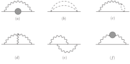
At one loop, only one non–vanishing diagram arises, which is a fermion exchange across the cusp point, as depicted in figure 6.
Throughout this computation, the contributions from the two diagonal blocks of the supermatrix (2.3) are the same and their sum simply cancels the factor 2 in the overall normalization (2.1). Parametrizing the points on the cusp line as , the algebra of the diagram gives
| (4.1) |
with . According to the method outlined above, we Fourier transform this to momentum space. Introducing the exponential IR regulator , we obtain
| (4.2) |
In the last line, the squared propagator arises from the two sides of the cusp which degenerate to the same HQET propagator in the limit.
We set and absorb the imaginary unit in the HQET propagator into the velocity . The resulting imaginary vector with is suitable for the evaluation of the master integrals in euclidean space, making them manifestly real.
Then we make use of identity (E.3d) to express the –bilinear in terms of the external velocity . This gives rise to the dependence of the diagram, according to (E.3b), and expresses the numerator of the integrand as . This in turn can be rewritten as an inverse HQET propagator, so that at this stage the diagram can be expressed as a linear combination of scalar HQET one-loop integrals (F)
| (4.3) |
where . An integration–by–parts identity allows to express everything only in terms of the master integral
| (4.4) |
Finally, using formula (F.7) we expand this integral in up to order as required by the three–loop computation and obtain the one–loop 1PI HQET vertex correction at zero cusp angle
| (4.5) |
up to an overall factor , omitted to keep the expression compact.
At two loops the relevant diagrams are shown in figure 7.
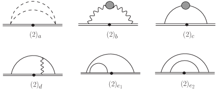
In general, each topology of diagrams is associated to a number of independent 1PI configurations, according to the position of the cusp point. Different configurations give rise to different powers of . As an example, in figure 7 we depict the two possible configurations of diagrams with double fermion exchanges, and , which give contributions proportional to and , respectively.
All the diagrams are computed in the HQET framework, following what have been described above for the one–loop case. The integration–by–parts reduction lands on to two master integrals only, which are defined and evaluated in appendix F. The list of results for each individual diagram is given in appendix G. Combining these expressions and expanding them up to order leads to the following (unrenormalized) expectation value of the 1PI part for the cusped WL at two loops
| (4.6) |
once again, omitting a factor . We stress that no sub–leading corrections in arise up to two loops.
5 Three loop calculation
5.1 Diagrams
At three loops it is convenient to classify the diagrams according to the number of fermion and scalar insertions. We provide only a sketch of the possible topologies of diagrams arising in the computation, but each of them can contribute with several different relative positions of the insertion and the cusp points, all giving rise to 1PI configurations, and/or different choices of the gauge vectors, or .
The planar diagrams can be organized according to
-
•
Diagrams containing scalar insertions, figure 8.
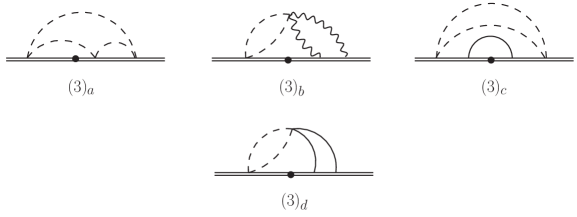
Figure 8: Diagrams with scalar insertions. is the only diagram obtained by contracting three bi–scalar insertions, with no fermion lines. This, along with diagram , does not actually contribute to the Bremsstrahlung function. In fact they possess a trivial dependence on the internal angle , as is immediate to infer using identities (E.3). Nonetheless, we take them into account in order to provide the full result for the cusp at vanishing angle.
Diagram comes in different configurations, each with a specific dependence, according to the relative positions between the insertions and the cusp point.
-
•
Diagrams with no scalar insertions and a fermion line attached to the WL, as depicted in figure 9.
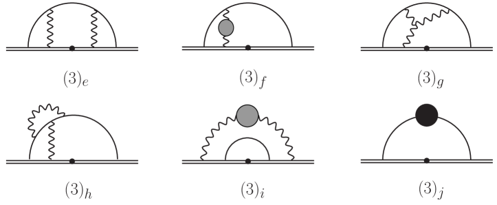
Figure 9: Diagrams with two fermion insertions. Grey and black bullets represent one and two loops self–energy corrections, respectively. Such diagrams arise in a variety of fashions, with up to three internal integration vertices. Several graphs feature lower order corrections to the field propagators. We recall that the one–loop correction to the scalar two–point function vanishes identically and the one for the fermion line (C.8) is proportional to the difference between the ranks of the two gauge groups, hence it vanishes in the ABJM theory. Diagrams and involve the one–loop gluon self–energy correction, whose result is reviewed in appendix C. In our computation we employed an effective propagator in momentum space with an unintegrated scalar bubble, in order to make the corresponding cusp contribution fit into the integral classification (F). Diagram contains the two–loop self–energy correction of the fermion propagator. Its computation in configuration space is spelled out in appendix D.
-
•
Diagrams with four fermion insertions along the line, as drawn in figure 10.
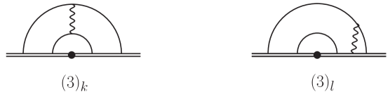
Figure 10: Diagrams with four fermion insertions. The topologies and possess 4 and 5 different inequivalent 1PI vertex configurations, respectively, among which we displayed explicitly two representatives.
-
•
Diagrams with three fermion lines departing and landing on the Wilson line, as pictured in figure 11.
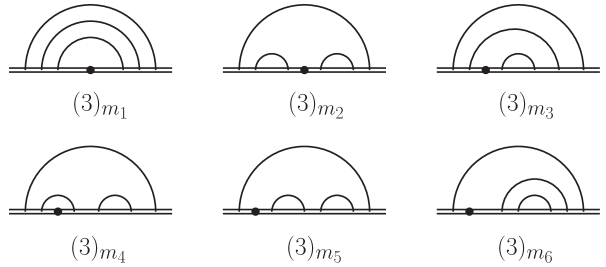
Figure 11: Fermion ladder diagrams. These are all ladder contributions with no internal integrations, making their evaluation easier than the previous contributions. In the cartoon we have only represented all possible 1PI vertex contractions, which are relevant for our computation.
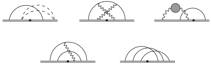
Finally, nonplanar diagrams can be constructed starting from the same field insertions as in graphs , , , , . These are sketched in figure 12.
5.2 The computation
We tackle the evaluation of three–loop Feynman diagrams by applying the HQET method described in section 3. The integrands related to the diagrams listed in the previous section can be computed using the Feynman rules in appendix C or using the Mathematica® package WiLE Preti:2017 . Since the complete calculation is quite long and cumbersome, here we spell out the explicit details of one particular diagram.
As an example, we consider diagram , selecting in particular the configuration drawn in figure 9 plus the one where the gluon insertion on the contour and the cusp point are interchanged. The two configurations, being symmetric and thus equivalent, yield an overall factor 2. To be definite, we call the sum of these two configurations . Further possible configurations from the topology arise, which correspond to other orderings of insertion points on the contour.
Considering configurations , we may obtain leading and sub–leading contributions, depending whether the gauge lines correspond to or .
We start computing the planar contributions. The starting string in configuration space is given by
| (5.1) |
where the constant factor reads
| (5.2) |
Next, we Fourier transform this expression using (C.1) (which eats up part of ) and arrive to an equivalent HQET–like contribution
| (5.3) |
where we have already introduced the IR regulator .
Next we use (E.3d) to reduce the –bilinear and extract the corresponding dependence. We perform the tensor algebra within the DRED scheme, using in particular a repeated (automatized) application of (A.2) to simplify the product of matrices to products of metrics and Levi–Civita tensors. In this process we discard all the contributions proportional to one final tensor, as it is doomed to vanish after integration, as explained in section 3.1. The result of this procedure leads to a numerator which can be expressed in terms of scalar products between integrated momenta and external velocities only. It looks like
As a final step, we rewrite the above expression in terms of inverse propagators and arrive at a sum of scalar integrals with different powers of the propagators, in a form which FIRE can be fed with. After the FIRE digestion, the diagram evaluates to a simple sum over the master integrals listed in appendix F
| (5.4) |
which can directly be expanded in to the desired order
| (5.5) |
Repeating the exercise for all the diagrams we obtain the results listed in appendix H.
We compute the nonplanar corrections as well, which are produced by two possible sources. At first they can come from planar diagrams, when for instance the choice of the vector boson gives rise to a sub–leading in color contraction of the color matrices. Second, they can be produced by genuinely nonplanar diagrams. We remark that, since we consider color subleading contributions, we also have to take into account the mixed gauge propagator contribution (C.7), arising at one–loop from the creation and annihilation of a matter pair.
The first class of contributions arises from diagrams , , , , , , and , whereas genuine nonplanar Wick contractions arise in topologies , , , and . Examples of such graphs are shown in figure 12, where we have shown only one particular nonplanar configuration for each topology. Thanks to the linear nature of the HQET propagators as functions of loop momenta, such nonplanar integrals contain linearly dependent propagators. These can be manipulated by partial fractioning (using an automated routine) in such a way to reduce them all to either planar integrals or a single nonplanar topology depicted in figure 15, with arbitrary powers of the propagators. These can be finally reduced by integration–by–parts identities to a single nonplanar master integral, which is defined and computed in appendix F. In particular, after decomposition by partial fractioning, the nonplanar diagrams arising from topologies and evaluate to planar integrals. Only diagrams , and give rise to the nonplanar topology of figure 15.
6 The three–loop cusp and the Bremsstrahlung function
We are now ready to provide the full result for the 1/2–BPS cusp anomalous dimension up to three loops, at vanishing geometric angle . Omitting an overall factor , the sum of all the three–loop contributions to the 1PI vertex function reads
| (6.1) | ||||
As a first consistency check of the result, we probe exponentiation (2.8). This test was already successfully performed up to two loops in Griguolo:2012iq and here we extend the analysis to the next perturbative order. To this end we insert the explicit expressions (4.5, 4.6, 6.1) for in the general expansion for the vertex function (3.10). Now, taking the logarithm and expand the resulting expression in powers of we do find
| (6.2) |
Although the and coefficients originally contained higher order poles in , only single poles appear in (6). This proves that quadratic and cubic poles in and , eqs. (4.6, 6.1), are ascribable to powers of lower order divergent contributions to . Therefore, as expected, the divergent part of the expectation value of the cusped WL exponentiates. In particular, since no nonplanar corrections appear at one– and two–loop orders, their contribution at three loops has only a simple pole in the regulator.
We note that the two–loop part in (6) is independent of . Applying prescription (3.7) to obtain the whole expression for the cusped WL this contribution will then get removed. The final result for the (unrenormalized) cusped WL at reads
| (6.3) |
This expression displays uniform transcendentality. Moreover, it satisfies the BPS condition, namely it vanishes for , albeit this statement is quite trivial at , being it an obvious consequence of (3.7).
As a further consistency check, we have also directly verified prescription (3.7) by computing the non–1PI contributions as well.
We renormalize (6.3) by multiplying by a renormalization function . Following the steps outlined in section 3.3, from we obtain the final result for the anomalous dimension at three loops
| (6.4) |
The Bremsstrahlung function is finally evaluated according to (3.12) and reads
| (6.5) |
This result is in perfect agreement with conjecture (2.13) that was formulated in Lewkowycz:2013laa ; Bianchi:2014laa . In fact, using the expectation value for the 1/6–BPS WLs at framing one, as derived from localization
| (6.6) |
and inserting them in the r.h.s. of (2.13) we find exactly expression (6.5). Remarkably, the agreement applies also to the nonplanar part. This is consistent with the fact that up to three loops the arguments of Bianchi:2014laa do not rely on restricting to the planar limit.
7 Conclusions
In this paper we have studied the Bremsstrahlung function for the locally 1/2–BPS cusp in the ABJM model at weak coupling with the aim of proving conjecture (2.13) for its exact determination. We remind that this conjecture is based on linking the Bremsstrahlung function to the expectation value of supersymmetric 1/6–BPS WLs with multiple winding, which are computable exactly via localization Klemm:2012ii . To begin with, it relies on the expectation values of supersymmetric WLs on latitude contours in (see eq. (2.10)) and hinges on a few steps, some of which lack a rigorous proof. Therefore, in order to substantiate the conjecture, we have performed a precision perturbative check at three loops.
Technically, we have taken considerable advantage from the BPS condition for the cusp, in order to make the computation simpler. We have considered the expansion of the cusp anomalous dimension in the small internal angle in the R–symmetry space, at vanishing geometric angle. This setting entails several simplifications at both the level of the diagrams involved, and in their practical evaluation, especially in handling the integrals. These reduce to propagator–type integrals, which we computed by switching to the HQET picture (via Fourier transform to momentum space) and employing integration by parts identities to reduce them to a restricted set of master topologies.
Result (6.5) for the three–loop Bremsstrahlung function agrees with the prediction based on conjecture (2.13). Remarkably, such an agreement extends to the nonplanar part as well. This provides a compelling test in favour of proposal (2.13) and its validity beyond the planar limit.
This exact result is interesting per se, but acquires additional appeal in view of a potential integrability based computation of the same quantity. Recent developments on the Quantum Spectral Curve approach Gromov:2013pga ; Gromov:2014caa ; Gromov:2015dfa ; Gromov:2016rrp in the ABJM model Cavaglia:2014exa ; Bombardelli:2017vhk seem to point to such a possibility. This would provide a crossed check of the localization based proposal and, by comparison with the integrable description, of the conjecture on the exact expression for the interpolating function of ABJM Nishioka:2008gz ; Grignani:2008is ; Gaiotto:2008cg ; Gromov:2014eha .
We conclude with comments on future perspectives and extensions of this paper.
A first, sensible generalization of the three–loop computation of the cusped 1/2–BPS WL consists in lifting the ranks of the two gauge groups to unequal values, or in other words to compute the same quantity in the ABJ model. From the technical standpoint, this requires modifying the color factors of the diagrams analysed in this article and supplying further graphs which were discarded, because they vanish in the ABJM limit.
Despite the fact that such a result is expected to be straightforward to derive, lower order contributions suggest that the expectation value of the locally 1/2–BPS WL on a cusped contour does not exponentiate Griguolo:2012iq ; Bonini:2016fnc , at least not in a standard fashion. This might hamper the interpretation of the three–loop correction and the extraction of a cusp anomalous dimension from it. Moreover, it is not clear if and how conjecture (2.10) can be extended to the case with different ranks. Still, the ABJ theory is expected to be integrable (it was proven to be so in a particular sector in the limit of Bianchi:2016rub ), therefore a derivation of its Bremsstrahlung function from integrability is also foreseeable. This, together with a deeper understanding of the ABJ supersymmetric cusp, would grant a firmer handle on the conjecture for the exact interpolating function of the ABJ model Cavaglia:2016ide . In conclusion, the lifting to the ABJ theory is challenging and requires more thinking, but is certainly an interesting direction to pursue.
In this paper we have found the exact expression of a cusped 1/2–BPS WL at three loops and at finite , eq. (6.3). A natural extension of this computation is the evaluation of the same 1/2–BPS cusp, but with open geometric angle (), along the lines of Grozin:2015kna . This task, if performed using the HQET description, demands the evaluation of the 71 master integrals pointed out in Grozin:2015kna , in three dimensions. However, this should be simpler than in four dimensions, as the leading divergence of the cusp integrals at loop is a pole of order in three dimensions, instead of in four. Consequently, the relevant integrals should be expanded up to terms of transcendentality 2 in the three loop case (compared to transcendental order 5). We have preliminary evidence that some of the master integrals required for the computation do not evaluate to generalized polylogarithms, rather elliptic sectors appear. Elliptic functions are likely to pop up at higher order in the –expansion or they might cancel out when summing all the diagrams, yet their presence can hinder the evaluation of the master integrals. In particular, at a difference with respect to the four dimensional case, we expect that a canonical form Henn:2013pwa does not exist for all of them.
Acknowledgements.
S.P. thanks the Galileo Galilei Institute for Theoretical Physics (GGI) for the hospitality and INFN for partial support during the completion of this work, within the program “New Developments in AdS3/CFT2 Holography”. This work has been supported in part by Italian Ministero dell’Istruzione, Università e Ricerca (MIUR), Della Riccia Foundation and Istituto Nazionale di Fisica Nucleare (INFN) through the “Gauge Theories, Strings, Supergravity” (GSS) and “Gauge And String Theory” (GAST) research projects.Appendix A Spinor and group conventions
We work in euclidean three dimensional space with coordinates . The Dirac matrices satisfying the Clifford algebra are chosen to be
| (A.1) |
with matrix product
| (A.2) |
The set of matrices (A.1) satisfies satisfies the following set of identities
| (A.3) | |||
which allows us to simplify the fermionic contributions to the WL. The relevant traces are instead given by
| (A.4) |
Spinor indices are raised and lowered by means of the tensor:
| (A.5) |
with . In particular, the antisymmetric combination of two spinors can be reduced to scalar contractions:
| (A.6) |
The gamma matrices with two lower indices, , are then given by
| (A.7) |
and they obey the useful identity.
| (A.8) |
Under complex conjugation the gamma matrices transform as follows: . As a consequence, the hermitian conjugate of the vector bilinear can be rewritten as follows
| (A.9) |
where we have taken and .
The U generators are defined as , where and () are an orthonormal set of traceless hermitian matrices. The generators are normalized as
| (A.10) |
The structure constant are then defined by
| (A.11) |
In the paper we shall often use the double notation and the fields will carry two indices in the fundamental representation of the gauge groups. An index in the fundamental representation of U will be generically by the lowercase roman indices , while for an index in the fundamental representation of U we shall use the hatted lowercase roman indices
Appendix B Basic facts on ABJM action
Here we collect some basic features on the action for general U U ABJ(M) theories. The gauge sector contains two gauge fields and belonging respectively to the adjoint of U and U. The matter sector instead consists of the complex fields and as well as the fermions and . The fields transform in the of the gauge group while the couple belongs to the representation . The additional capitol index belongs to the R–symmetry group . In order to quantize the theory at the perturbative level, we introduce the usual Feynman gauge–fixing for both gauge fields and the two corresponding sets of ghosts and . Then the action contains four different contributions
| (B.1) |
where
| (B.2a) | ||||
| (B.2b) | ||||
| (B.2c) | ||||
| (B.2d) | ||||
Here the invariant tensors and are defined by setting . The covariant derivatives used in (B.1) are instead given by
| (B.3) |
The action (B.1), in absence of the gauge-fixing terms and of the corresponding ghosts, it is invariant under the following SUSY transformations
| (B.4) |
Appendix C Feynman rules
We use the Fourier transform definition
| (C.1) |
From the action (B.1) we read the following Feynman rules666In euclidean space we define the functional generator as .
-
•
Vector propagators in Landau gauge
(C.2) -
•
Scalar propagator
(C.3) -
•
Fermion propagator
(C.4) -
•
Gauge cubic vertex
(C.5) -
•
Gauge-fermion cubic vertex
(C.6)
At one–loop, if we work at finite and , beside corrections to the tree level vector propagators, a contribution to the mixed propagator is generated. They read
| (C.7a) | ||||
| (C.7b) | ||||
| (C.7c) | ||||
The one-loop fermion propagator reads
| (C.8) | |||||
and is proportional to the difference of the ranks of the gauge groups. Hence it vanishes in the ABJM limit and is not needed in our computation.
Appendix D Two–loop self–energy corrections to the fermions
In this appendix we spell out the computation of the two–loop corrections to the fermion two–point functions. Throughout this section we work with different group ranks.
The relevant Feynman diagrams are depicted in figure 13.
Considering all the possible permutations, the contributions of the diagrams in figure 13 are given by
| (D.1) |
where
| (D.2) | ||||
| (D.3) | ||||
| (D.4) | ||||
| (D.5) | ||||
| (D.6) | ||||
| (D.7) |
Summing all the contributions we get
| (D.8) |
The reducible two-loop correction of figure 14 gives
| (D.9) |
Each correction to the fermion propagator can be Fourier transformed back to configuration space
| (D.10) |
Appendix E Useful identities on the cusp
We parametrize a point on the line forming the cusp as
| (E.1) |
Simple identities that turn out to be useful along the calculation are
| (E.2a) | |||
| (E.2b) | |||
| (E.2c) | |||
| (E.2d) | |||
The spinor couplings , for the fermions and the matrices for the scalars appearing in the superconnection (2.3) obey the identities (at )
| (E.3a) | ||||
| (E.3b) | ||||
| (E.3c) | ||||
| (E.3d) | ||||
| (E.3e) | ||||
| (E.3f) | ||||
| (E.3g) | ||||
| (E.3h) | ||||
| (E.3i) | ||||
| (E.3j) | ||||
Identity (E.3d), and the formulae above it, are widely used in the computation, since they apply whenever a diagram contains a fermion arch. Identities (E.3g) have been used in the diagrams with scalar insertions of figure 8, while identities (E.3j) are relevant for diagram .
Appendix F Master integrals definitions and expansions
We define the HQET planar integrals at one, two and three loops by the following products of propagators ()
| one loop: | ||||
| two loops: | ||||
| three loops: | (F.1) |
where the explicit propagators read
| (F.2) |
and . At three loops we also need to consider the non–planar topology
| (F.3) |
with propagators given by
| (F.4) |
At one loop there is only one master integral which can be chosen to be . The HQET bubble integral evaluates for generic indices
| (F.5) |
Fixing the index of the HQET and standard propagators to unity, this formula generalizes to multiloop bubble integrals by integrating bubble sub–topologies iteratively
| (F.6) |
where in the denominator we used the Pochhammer symbol . In view of the three–loop calculation we need the explicit expansion
| (F.7) |
omitting a factor .
At two loops two master integrals appear which we choose to be and . They can be expressed exactly in terms of the function introduced above
| (F.8) | ||||
| (F.9) |
These functions can be straightforwardly expanded in power series of
| (F.10) | ||||
| (F.11) |
omitting .
At three loops there are eight master integrals that, following Grozin:2000jv , we choose to be the ones in figure 15.
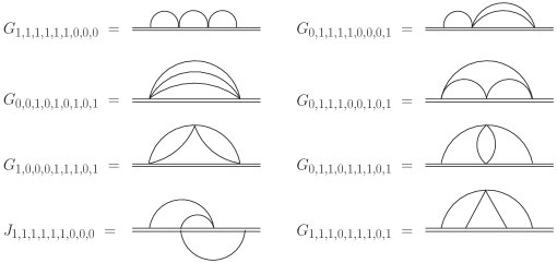
The master integrals can be evaluated in dimensions and expanded up to the needed order
where an overall factor is omitted.
Appendix G Results for two–loop diagrams
Here we provide the list of results for the two–loop diagrams of figure 7, considering only the 1PI configurations on the cusp.
| (G.1) | ||||
| (G.2) | ||||
| (G.3) | ||||
| (G.4) | ||||
| (G.5) |
A common factor is omitted.
Appendix H Results for three–loop diagrams
Here we list the results for the HQET-1PI part of the diagrams. The results include the nonplanar corrections and are already given by the sum over different configurations belonging to the same topology, following the classification of section 5.1. A common factor is understood.
| (H.1) | ||||
| (H.2) | ||||
| (H.3) | ||||
| (H.4) | ||||
| (H.5) | ||||
| (H.6) | ||||
| (H.7) | ||||
| (H.8) | ||||
| (H.9) | ||||
| (H.10) | ||||
| (H.11) | ||||
| (H.12) | ||||
| (H.13) | ||||
References
- (1) M. S. Bianchi, L. Griguolo, M. Leoni, S. Penati and D. Seminara, BPS Wilson loops and Bremsstrahlung function in ABJ(M): a two loop analysis, JHEP 06 (2014) 123, [1402.4128].
- (2) J. M. Maldacena, The Large N limit of superconformal field theories and supergravity, Adv.Theor.Math.Phys. 2 (1998) 231–252, [hep-th/9711200].
- (3) E. Witten, Anti-de Sitter space and holography, Adv. Theor. Math. Phys. 2 (1998) 253–291, [hep-th/9802150].
- (4) S. S. Gubser, I. R. Klebanov and A. M. Polyakov, Gauge theory correlators from non-critical string theory, Phys. Lett. B428 (1998) 105–114, [hep-th/9802109].
- (5) J. M. Maldacena, Wilson loops in large N field theories, Phys.Rev.Lett. 80 (1998) 4859–4862, [hep-th/9803002].
- (6) S.-J. Rey and J.-T. Yee, Macroscopic strings as heavy quarks in large N gauge theory and anti-de Sitter supergravity, Eur.Phys.J. C22 (2001) 379–394, [hep-th/9803001].
- (7) V. Pestun, Localization of gauge theory on a four-sphere and supersymmetric Wilson loops, Commun. Math. Phys. 313 (2012) 71–129, [0712.2824].
- (8) A. Kapustin, B. Willett and I. Yaakov, Exact Results for Wilson Loops in Superconformal Chern-Simons Theories with Matter, JHEP 1003 (2010) 089, [0909.4559].
- (9) J. Erickson, G. Semenoff and K. Zarembo, Wilson loops in supersymmetric Yang-Mills theory, Nucl.Phys. B582 (2000) 155–175, [hep-th/0003055].
- (10) N. Drukker and D. J. Gross, An Exact prediction of N=4 SUSYM theory for string theory, J. Math. Phys. 42 (2001) 2896–2914, [hep-th/0010274].
- (11) D. Correa, J. Henn, J. Maldacena and A. Sever, An exact formula for the radiation of a moving quark in N=4 super Yang Mills, JHEP 06 (2012) 048, [1202.4455].
- (12) N. Drukker, D. J. Gross and H. Ooguri, Wilson loops and minimal surfaces, Phys.Rev. D60 (1999) 125006, [hep-th/9904191].
- (13) N. Drukker and V. Forini, Generalized quark-antiquark potential at weak and strong coupling, JHEP 06 (2011) 131, [1105.5144].
- (14) D. Bombardelli, D. Fioravanti and R. Tateo, Thermodynamic Bethe Ansatz for planar AdS/CFT: A Proposal, J. Phys. A42 (2009) 375401, [0902.3930].
- (15) N. Gromov, V. Kazakov, A. Kozak and P. Vieira, Exact Spectrum of Anomalous Dimensions of Planar N = 4 Supersymmetric Yang-Mills Theory: TBA and excited states, Lett. Math. Phys. 91 (2010) 265–287, [0902.4458].
- (16) G. Arutyunov and S. Frolov, Thermodynamic Bethe Ansatz for the AdS(5) S(5) Mirror Model, JHEP 05 (2009) 068, [0903.0141].
- (17) D. Correa, J. Maldacena and A. Sever, The quark anti-quark potential and the cusp anomalous dimension from a TBA equation, JHEP 08 (2012) 134, [1203.1913].
- (18) N. Drukker, Integrable Wilson loops, JHEP 10 (2013) 135, [1203.1617].
- (19) N. Gromov and A. Sever, Analytic Solution of Bremsstrahlung TBA, JHEP 11 (2012) 075, [1207.5489].
- (20) N. Gromov, F. Levkovich-Maslyuk and G. Sizov, Analytic Solution of Bremsstrahlung TBA II: Turning on the Sphere Angle, JHEP 10 (2013) 036, [1305.1944].
- (21) M. Bonini, L. Griguolo, M. Preti and D. Seminara, Bremsstrahlung function, leading Lüscher correction at weak coupling and localization, JHEP 02 (2016) 172, [1511.05016].
- (22) N. Gromov, V. Kazakov, S. Leurent and D. Volin, Quantum Spectral Curve for Planar Super-Yang-Mills Theory, Phys. Rev. Lett. 112 (2014) 011602, [1305.1939].
- (23) N. Gromov, V. Kazakov, S. Leurent and D. Volin, Quantum spectral curve for arbitrary state/operator in AdS5/CFT4, JHEP 09 (2015) 187, [1405.4857].
- (24) N. Gromov and F. Levkovich-Maslyuk, Quantum Spectral Curve for a cusped Wilson line in SYM, JHEP 04 (2016) 134, [1510.02098].
- (25) B. Fiol, E. Gerchkovitz and Z. Komargodski, Exact Bremsstrahlung Function in Superconformal Field Theories, Phys. Rev. Lett. 116 (2016) 081601, [1510.01332].
- (26) O. Aharony, O. Bergman, D. L. Jafferis and J. Maldacena, superconformal Chern-Simons-matter theories, M2-branes and their gravity duals, JHEP 0810 (2008) 091, [0806.1218].
- (27) O. Aharony, O. Bergman and D. L. Jafferis, Fractional M2-branes, JHEP 0811 (2008) 043, [0807.4924].
- (28) D. Berenstein and D. Trancanelli, Three-dimensional SCFT’s and their membrane dynamics, Phys. Rev. D78 (2008) 106009, [0808.2503].
- (29) N. Drukker, J. Plefka and D. Young, Wilson loops in 3-dimensional N=6 supersymmetric Chern-Simons Theory and their string theory duals, JHEP 11 (2008) 019, [0809.2787].
- (30) B. Chen and J.-B. Wu, Supersymmetric Wilson Loops in N=6 Super Chern-Simons-matter theory, Nucl. Phys. B825 (2010) 38–51, [0809.2863].
- (31) S.-J. Rey, T. Suyama and S. Yamaguchi, Wilson Loops in Superconformal Chern-Simons Theory and Fundamental Strings in Anti-de Sitter Supergravity Dual, JHEP 0903 (2009) 127, [0809.3786].
- (32) N. Drukker and D. Trancanelli, A Supermatrix model for N=6 super Chern-Simons-matter theory, JHEP 02 (2010) 058, [0912.3006].
- (33) L. Griguolo, D. Marmiroli, G. Martelloni and D. Seminara, The generalized cusp in ABJ(M) N = 6 Super Chern-Simons theories, JHEP 05 (2013) 113, [1208.5766].
- (34) A. Lewkowycz and J. Maldacena, Exact results for the entanglement entropy and the energy radiated by a quark, JHEP 05 (2014) 025, [1312.5682].
- (35) M. Marino and P. Putrov, Exact Results in ABJM Theory from Topological Strings, JHEP 1006 (2010) 011, [0912.3074].
- (36) N. Drukker, M. Marino and P. Putrov, From weak to strong coupling in ABJM theory, Commun.Math.Phys. 306 (2011) 511–563, [1007.3837].
- (37) V. Forini, V. G. M. Puletti and O. Ohlsson Sax, The generalized cusp in and more one-loop results from semiclassical strings, J. Phys. A46 (2013) 115402, [1204.3302].
- (38) J. Aguilera-Damia, D. H. Correa and G. A. Silva, Semiclassical partition function for strings dual to Wilson loops with small cusps in ABJM, JHEP 03 (2015) 002, [1412.4084].
- (39) D. H. Correa, J. Aguilera-Damia and G. A. Silva, Strings in Wilson loops in 6 super Chern-Simons-matter and bremsstrahlung functions, JHEP 06 (2014) 139, [1405.1396].
- (40) G. P. Korchemsky and A. V. Radyushkin, Renormalization of the Wilson Loops Beyond the Leading Order, Nucl. Phys. B283 (1987) 342–364.
- (41) J.-L. Gervais and A. Neveu, The Slope of the Leading Regge Trajectory in Quantum Chromodynamics, Nucl. Phys. B163 (1980) 189–216.
- (42) V. S. Dotsenko and S. N. Vergeles, Renormalizability of Phase Factors in the Nonabelian Gauge Theory, Nucl. Phys. B169 (1980) 527–546.
- (43) I. Ya. Arefeva, Quantum Contour Field Equations, Phys. Lett. B93 (1980) 347–353.
- (44) J. G. M. Gatheral, Exponentiation of Eikonal Cross-sections in Nonabelian Gauge Theories, Phys. Lett. B133 (1983) 90–94.
- (45) A. Klemm, M. Marino, M. Schiereck and M. Soroush, Aharony-Bergman-Jafferis-Maldacena Wilson loops in the Fermi gas approach, Z. Naturforsch. A68 (2013) 178–209, [1207.0611].
- (46) M. S. Bianchi, L. Griguolo, M. Leoni, A. Mauri, S. Penati and D. Seminara, Framing and localization in Chern-Simons theories with matter, JHEP 06 (2016) 133, [1604.00383].
- (47) M. S. Bianchi, L. Griguolo, M. Leoni, A. Mauri, S. Penati and D. Seminara, The quantum 1/2 BPS Wilson loop in Chern-Simons-matter theories, JHEP 09 (2016) 009, [1606.07058].
- (48) K. G. Chetyrkin, A. L. Kataev and F. V. Tkachov, New Approach to Evaluation of Multiloop Feynman Integrals: The Gegenbauer Polynomial Space Technique, Nucl. Phys. B174 (1980) 345–377.
- (49) A. Mauri, A. Santambrogio and S. Scoleri, The Leading Order Dressing Phase in ABJM Theory, JHEP 04 (2013) 146, [1301.7732].
- (50) A. Grozin, J. M. Henn, G. P. Korchemsky and P. Marquard, Three Loop Cusp Anomalous Dimension in QCD, Phys. Rev. Lett. 114 (2015) 062006, [1409.0023].
- (51) A. Grozin, J. M. Henn, G. P. Korchemsky and P. Marquard, The three-loop cusp anomalous dimension in QCD and its supersymmetric extensions, JHEP 01 (2016) 140, [1510.07803].
- (52) W. Siegel, Supersymmetric Dimensional Regularization via Dimensional Reduction, Phys. Lett. B84 (1979) 193–196.
- (53) M. Bianchi, G. Giribet, M. Leoni and S. Penati, The 1/2 BPS Wilson loop in ABJ(M) at two loops: The details, JHEP 1310 (2013) 085, [1307.0786].
- (54) L. Griguolo, G. Martelloni, M. Poggi and D. Seminara, Perturbative evaluation of circular 1/2 BPS Wilson loops in 6 Super Chern-Simons theories, JHEP 1309 (2013) 157, [1307.0787].
- (55) M. S. Bianchi, G. Giribet, M. Leoni and S. Penati, Light-like Wilson loops in ABJM and maximal transcendentality, JHEP 08 (2013) 111, [1304.6085].
- (56) A. G. Grozin, Calculating three loop diagrams in heavy quark effective theory with integration by parts recurrence relations, JHEP 03 (2000) 013, [hep-ph/0002266].
- (57) K. G. Chetyrkin and A. G. Grozin, Three loop anomalous dimension of the heavy light quark current in HQET, Nucl. Phys. B666 (2003) 289–302, [hep-ph/0303113].
- (58) F. V. Tkachov, A Theorem on Analytical Calculability of Four Loop Renormalization Group Functions, Phys. Lett. B100 (1981) 65–68.
- (59) K. G. Chetyrkin and F. V. Tkachov, Integration by Parts: The Algorithm to Calculate beta Functions in 4 Loops, Nucl. Phys. B192 (1981) 159–204.
- (60) S. Laporta and E. Remiddi, The Analytical value of the electron (g-2) at order alpha**3 in QED, Phys. Lett. B379 (1996) 283–291, [hep-ph/9602417].
- (61) S. Laporta, High precision calculation of multiloop Feynman integrals by difference equations, Int. J. Mod. Phys. A15 (2000) 5087–5159, [hep-ph/0102033].
- (62) A. V. Smirnov, Algorithm FIRE – Feynman Integral REduction, JHEP 10 (2008) 107, [0807.3243].
- (63) A. V. Smirnov and V. A. Smirnov, FIRE4, LiteRed and accompanying tools to solve integration by parts relations, Comput. Phys. Commun. 184 (2013) 2820–2827, [1302.5885].
- (64) A. V. Smirnov, FIRE5: a C++ implementation of Feynman Integral REduction, Comput. Phys. Commun. 189 (2015) 182–191, [1408.2372].
- (65) R. N. Lee, Presenting LiteRed: a tool for the Loop InTEgrals REDuction, 1212.2685.
- (66) R. N. Lee, LiteRed 1.4: a powerful tool for reduction of multiloop integrals, J. Phys. Conf. Ser. 523 (2014) 012059, [1310.1145].
- (67) K.-M. Lee and S. Lee, 1/2-BPS Wilson Loops and Vortices in ABJM Model, JHEP 09 (2010) 004, [1006.5589].
- (68) M. Lietti, A. Mauri, S. Penati and J.-j. Zhang, String theory duals of Wilson loops from Higgsing, 1705.02322.
- (69) H. Dorn, Renormalization of Path Ordered Phase Factors and Related Hadron Operators in Gauge Field Theories, Fortsch. Phys. 34 (1986) 11–56.
- (70) N. S. Craigie and H. Dorn, On the Renormalization and Short Distance Properties of Hadronic Operators in QCD, Nucl. Phys. B185 (1981) 204–220.
- (71) S. Aoyama, The Renormalization of the String Operator in QCD, Nucl. Phys. B194 (1982) 513–534.
- (72) D. Knauss and K. Scharnhorst, Two Loop Renormalization of Nonsmooth String Operators in Yang-Mills Theory, Annalen Phys. 41 (1984) 331–344.
- (73) M. Preti, WiLE: a Mathematic package for weak coupling expansion of Wilson loops in ABJ(M) theory, to appear (2017) .
- (74) N. Gromov and F. Levkovich-Maslyuk, Quark-anti-quark potential in 4 SYM, JHEP 12 (2016) 122, [1601.05679].
- (75) A. Cavaglià, D. Fioravanti, N. Gromov and R. Tateo, Quantum Spectral Curve of the 6 Supersymmetric Chern-Simons Theory, Phys. Rev. Lett. 113 (2014) 021601, [1403.1859].
- (76) D. Bombardelli, A. Cavaglià, D. Fioravanti, N. Gromov and R. Tateo, The full Quantum Spectral Curve for , 1701.00473.
- (77) T. Nishioka and T. Takayanagi, On Type IIA Penrose Limit and N=6 Chern-Simons Theories, JHEP 08 (2008) 001, [0806.3391].
- (78) G. Grignani, T. Harmark and M. Orselli, The SU(2) SU(2) sector in the string dual of N=6 superconformal Chern-Simons theory, Nucl. Phys. B810 (2009) 115–134, [0806.4959].
- (79) D. Gaiotto, S. Giombi and X. Yin, Spin Chains in N=6 Superconformal Chern-Simons-Matter Theory, JHEP 04 (2009) 066, [0806.4589].
- (80) N. Gromov and G. Sizov, Exact Slope and Interpolating Functions in N=6 Supersymmetric Chern-Simons Theory, Phys. Rev. Lett. 113 (2014) 121601, [1403.1894].
- (81) M. Bonini, L. Griguolo, M. Preti and D. Seminara, Surprises from the resummation of ladders in the ABJ(M) cusp anomalous dimension, JHEP 05 (2016) 180, [1603.00541].
- (82) M. S. Bianchi and M. Leoni, An exact limit of the Aharony-Bergman-Jafferis-Maldacena theory, Phys. Rev. D94 (2016) 045011, [1605.02745].
- (83) A. Cavaglià, N. Gromov and F. Levkovich-Maslyuk, On the Exact Interpolating Function in ABJ Theory, JHEP 12 (2016) 086, [1605.04888].
- (84) J. M. Henn, Multiloop integrals in dimensional regularization made simple, Phys.Rev.Lett. 110 (2013) 251601, [1304.1806].