.
Accuracy of Estimating Highly Eccentric Binary Black Hole Parameters With Gravitational-Wave Detections
Abstract
Mergers of stellar-mass black holes on highly eccentric orbits are among the targets for ground-based gravitational-wave detectors, including LIGO, VIRGO, and KAGRA. These sources may commonly form through gravitational-wave emission in high velocity dispersion systems or through the secular Kozai-Lidov mechanism in triple systems. Gravitational waves carry information about the binaries’ orbital parameters and source location. Using the Fisher matrix technique, we determine the measurement accuracy with which the LIGO-VIRGO-KAGRA network could measure the source parameters of eccentric binaries using a matched filtering search of the repeated burst and eccentric inspiral phases of the waveform. We account for general relativistic precession and the evolution of the orbital eccentricity and frequency during the inspiral. We find that the signal-to-noise ratio and the parameter measurement accuracy may be significantly higher for eccentric sources than for circular sources. This increase is sensitive to the initial pericenter distance, the initial eccentricity, and component masses. For instance, compared to a non-spinning circular binary, the chirp mass and sky localization accuracy can improve for an initially highly eccentric binary by a factor of () and () assuming an initial pericenter distance of ().
Subject headings:
black hole physics – gravitational waves1. Introduction
The Advanced Laser Interferometer Gravitational Wave Observatory111http://www.ligo.caltech.edu/ (aLIGO) detectors (Aasi et al., 2015) and Advanced Virgo222http://www.ego-gw.it/ (AdV) (Acernese et al., 2015) have made the first six detections of GWs from approximately circular inspiraling binaries (Abbott et al., 2016c, d, 2017a, 2017b, 2017c, 2017d), and opened a new window through which to observe the universe. These advanced gravitational-wave (GW) detectors together with upcoming instruments KAGRA333http://gwcenter.icrr.u-tokyo.ac.jp/en/ (Somiya, 2012) and LIGO-India444http://www.gw-indigo.org/ (Iyer et al., 2011; Abbott et al., 2016f) are expected to continue to detect GW sources in the upcoming years (Abbott et al., 2016f). The orbital eccentricity was neglected in the analysis of the detected GW sources, but a preliminary upper limit was claimed to be at 10 Hz (Abbott et al., 2016a, e, 2017a, 2017e). In this paper we estimate the future potential of the aLIGO-AdV-KAGRA network of advanced GW detectors to measure the orbital eccentricity and other physical parameters of initially highly eccentric sources.
Initially highly eccentric black hole (BH) binaries are inspiraling systems, which have orbital eccentricities beyond when their peak GW frequency (Wen, 2003) enters the sensitive frequency band of advanced Earth-based GW detectors. The orbital eccentricity decreases in the inspiral phase from this value until the last stable orbit (LSO) (Peters, 1964). Such systems can form in multiple ways including single-single encounters due to GW emission (Kocsis et al., 2006b; O’Leary et al., 2009; Gondán et al., 2017) in dense, high-velocity-dispersion environments; dynamical multibody interactions (Gültekin et al., 2006; O’Leary et al., 2006; Kushnir et al., 2013; Amaro-Seoane & Chen, 2016; Antonini & Rasio, 2016; Rodriguez et al., 2017); the secular Kozai-Lidov mechanism (Wen, 2003; Thompson, 2011; Aarseth, 2012; Antonini & Perets, 2012; Antognini et al., 2014; Antonini et al., 2014, 2016; Breivik et al., 2016; Rodriguez et al., 2016a, b; VanLandingham et al., 2016; Hoang et al., 2017; Petrovich & Antonini, 2017; Silsbee & Tremaine, 2017; Randall & Xianyu, 2018) in hierarchical triples, or the binary-single interaction (Samsing et al., 2014; Samsing & Ramirez-Ruiz, 2017; Samsing, 2017; Samsing et al., 2017). Eccentric BH binaries offer promising new detection candidates.
Previous parameter estimation studies of stellar-mass compact binaries have mostly focused on circular binaries (see Finn 1992; Finn & Chernoff 1993; Marković 1993; Cutler & Flanagan 1994; Jaranowski & Krolak 1994; Kokkotas et al. 1994; Królak et al. 1995; Poisson & Will 1995 for the first papers and Chatziioannou et al. 2014; Favata 2014; Mandel et al. 2014; O’Shaughnessy et al. 2014; Rodriguez et al. 2014; Canizares et al. 2015; Veitch et al. 2015; Berry et al. 2015; Miller et al. 2015; Farr et al. 2016; Moore et al. 2016; Lange et al. 2017; Vitale et al. 2017 for recent developments) due to their predicted high detection rates. The current detections constrain the merger rate density of BH-BH mergers in the Universe to (Abbott et al., 2017a), which corresponds to a detection rate between for a typical detection range for aLIGOs design sensitivity. Furthermore, see Abadie et al. (2010) for a partial list of historical compact binary coalescence rate predictions, and Dominik et al. (2013); Kinugawa et al. (2014); Abbott et al. (2016a, b, h, i, g); Belczynski et al. (2016); Rodriguez et al. (2016a); Bartos et al. (2017); McKernan et al. (2017); Hoang et al. (2017); Stone et al. (2017) and references therein for recent rate estimates.
However, several theoretical studies have shown that the detection rates of highly eccentric BH binaries may be non-negligible. For sources formed by GW-emission in galactic nuclei (GNs), the expected aLIGO detection rate at design sensitivity may be higher than if the BH mass function extends to masses above (O’Leary et al., 2009; Kocsis & Levin, 2012). Recently, such heavy BHs have been observed in several LIGO/VIRGO detections (Abbott et al., 2016b, 2017a, 2017c). Additionally, the expected merger rate densities in the Kozai-Lidov channel are for BH binaries forming in nuclear star clusters without supermassive BHs (SMBHs) through multi-body interactions (Antonini & Rasio, 2016) and in isolated triple systems (Silsbee & Tremaine, 2017). Of order merger rate density is expected for BH binaries forming via the Kozai-Lidov mechanism in globular clusters (Antonini et al., 2014, 2016; Rodriguez et al., 2016a) and in GNs (Antonini & Perets, 2012; Hoang et al., 2017), and non-spherical nuclear star clusters may produce BH binary merger rates of up to (Petrovich & Antonini, 2017). Smaller size GNs with intermediate mass BHs may produce higher rates (VanLandingham et al., 2016). Binary-single gravitational interactions may greatly increase the rates (Samsing et al., 2014; Samsing & Ramirez-Ruiz, 2017; Samsing, 2017; Samsing et al., 2017). In a companion paper (Gondán et al., 2017), we have shown that GW capture sources in galactic nuclei, which appear to be circular to within near the LSO, may be highly eccentric at the beginning of the detected waveform at , and that heavier BH binaries are expected to be systematically more eccentric in this channel. The ongoing development of detectors towards their design sensitivity at low frequencies may open the possibility of detecting eccentricity in such systems.
In this paper, we determine the expected accuracy with which a network of ground-based interferometric GW detectors may determine the physical parameters that describe highly eccentric BH binaries in comparison to circular sources. We investigate how signal-to-noise ratios (SNRs) and parameter measurement errors depend on the initial orbital parameters, particularly the initial pericenter distance and eccentricity. We examine if it is possible to measure the initial binary parameters (initial eccentricity and pericenter distance) at formation for sources that form in the GW frequency band of the instrument.
Previous GW parameter estimation accuracy studies for eccentric waveforms were carried out for extreme mass ratio (EMRI) sources around SMBHs for LISA (Barack & Cutler 2004; Porter & Sesana 2010; Cornish & Key 2010; Mikóczi et al. 2012; Nishizawa et al. 2016) and for low-eccentricity stellar-mass compact binaries for Earth-based GW detector network (Sun et al., 2015). The premerger localization accuracy of eccentric neutron star binary systems was determined by Kyutoku & Seto (2014), and the source localization accuracy was investigated for low-eccentricity binaries by Ma et al. (2017).
The parameter space of an eccentric spinning binary waveform is generally very large, 17-dimensional (Vecchio, 2004; Cornish & Key, 2010). Therefore, state-of-the-art methods such as Monte Carlo Markov Chain calculations (see O’Shaughnessy et al. 2014 and references therein) are numerically prohibitively expensive to explore the full range of source parameters for a large set of binaries. For Gaussian noise and a large SNR, the posterior distribution function of the measured parameters is generally well approximated by a multidimensional Gaussian, and the parameter measurement errors can be estimated accurately and very efficiently using the Fisher matrix method (Finn & Chernoff, 1993; Cutler & Flanagan, 1994; Cutler & Vallisneri, 2007). Using this technique, we determine the physical parameters’ measurement accuracy.
We restrict this first study to waveforms introduced by Moreno-Garrido et al. (1994) and Moreno-Garrido et al. (1995), which account for part of the leading order post-Newtonian correction, the GR pericenter precession (hereafter simply precession) and neglect other first post-Newtonian and higher order corrections including those due to spins. Future extensions of this work should include higher order post-Newtonian and merger waveforms (see Levin et al. 2011; Csizmadia et al. 2012; East et al. 2013 for waveform generators, Damour et al. 2004; Memmesheimer et al. 2004; Königsdörffer & Gopakumar 2005, 2006; Yunes et al. 2009; Tessmer & Schäfer 2010, 2011; Huerta et al. 2014; Mikóczi et al. 2015; Moore et al. 2016; Tanay et al. 2016; Boetzel et al. 2017; Cao & Han 2017; Hinderer & Babak 2017; Huerta et al. 2017a, b; Loutrel & Yunes 2017 for analytic waveform models, and Hinder et al. 2008; East et al. 2012; Gold et al. 2012; Gold & Brügmann 2013; East et al. 2015; Paschalidis et al. 2015; East et al. 2016; Lewis et al. 2017 for waveforms of numerical relativity simulations of eccentric compact binary inspirals). In this paper, we focus on BH-BH binaries, but the method is also applicable for neutron star-neutron star and neutron star-black hole binaries on highly eccentric orbits as long as tidal interactions and matter exchange among the components are negligible (see Gold et al. 2012; East et al. 2015, 2016; Radice et al. 2016 and references therein). 555Eccentric neutron star (NS) binaries (NS-NS or NS-BH) will also benefit from additional information if an electromagnetic counterpart is identified, which may lead to smaller parameter errors (Radice et al., 2016).
Once a large number of GW sources is detected, the correlations between the orbital eccentricity, binary total mass, reduced mass, and spins may be distinctive among different astrophysical mechanisms leading to BH mergers (O’Leary et al., 2009; Cholis et al., 2016; Rodriguez et al., 2016a, b; Chatterjee et al., 2017; Gondán et al., 2017; Samsing & Ramirez-Ruiz, 2017; Silsbee & Tremaine, 2017; Kocsis et al., 2017). Therefore, detections of eccentric BH binaries have a potential in constraining GW source populations.
However, detecting eccentric sources and recovering their physical parameters is very challenging. So far three search methods were developed to find the signals of stellar-mass eccentric BH binaries in data streams of GW detectors (Tai et al., 2014; Coughlin et al., 2015; Tiwari et al., 2016). All three methods achieve substantially better sensitivity for eccentric BH binary signals than existing localized burst searches or chirp-like template based search methods. Once a source is detected, different algorithms are used to recover its physical parameters. For compact binary coalescences, BAYESTAR (Singer & Price, 2016) is an online fast sky localization algorithm that produces probability sky maps, LALInference (Veitch et al., 2015) is an offline full parameter estimation algorithm, and gstlal (Cannon et al., 2012; Privitera et al., 2014) is a low-latency binary BH parameter estimation algorithm. All three algorithms use waveform models of compact binaries on circular orbits. In addition, for short-duration GW ”bursts” with poorly modeled or unknown waveforms, Coherent WaveBurst (Klimenko et al., 2016), BayesWave (Cornish & Littenberg, 2015), and LALInferenceBurst (Veitch et al., 2015) pipelines produce reconstructed waveforms with minimal assumptions on the waveform morphology. The development of algorithms recovering the parameters of compact binaries on eccentric orbits are currently underway. These algorithms will play an important role for the astrophysical interpretation of eccentric sources.
The paper is organized as follows. In Section 2, we summarize the basic formulae describing the time-domain and frequency-domain eccentric waveform model. In Section 3, we outline the properties of advanced detectors we use in the analysis. In Section 4, we describe the signal parameter measurement estimation method. In Section 5, we discuss which parameters of an eccentric binary can be measured through the binary’s waveform. We present our main results in Section 6, and compare or results with previous papers. Finally, we summarize our conclusions in Section 7. Several details about our methodology is included in appendices. In Appendix A, we consider the values of source parameters in the circular limit. Next, in Appendix B, we introduce the geometric conventions we use to describe how the GWs interact with ground-based detectors. In Appendix C, we discuss the applicability of the assumptions of neglecting the Earth’s rotation around its axis and Earth’s motion around the Sun. In Appendix D, we derive numerically effective formulae to reduce the computational cost of numerical calculations of the and the Fisher matrix. In Appendix E, we present numerical comparisons to validate our codes for both precessing and non-precessing waveforms.
We use units when referring to the initial orbital parameters, and when determining the phases of waveforms. We work in the observer frame assuming a binary at cosmological redshift . In this frame, all of the formulae have redshifted mass parameters .666Additional corrections are necessary if the binary has a peculiar velocity (Kocsis et al., 2006a).
2. Eccentric Waveform Model
In this section, we summarize the basic formulae describing the time-domain (Section 2.1) and frequency-domain (Section 2.2) eccentric waveform models including precession in the leading quadrupole-order radiation approximation using the Fourier-Bessel decomposition. Note that we neglect the radiation of higher multipole orders, which are typically subdominant at least in cases where the initial pericenter distance is not close to a grazing or zoom-whirl configuration and the initial velocity is much less than the speed of light (Davis et al., 1972; Berti et al., 2010; Healy et al., 2016).
2.1. The waveform in time domain
We adopt the waveform model of Moreno-Garrido et al. (1994) and Moreno-Garrido et al. (1995), which describes the quadrupole waveform emitted by a spinless binary on a Keplerian orbit undergoing slow precession. For a fixed semi-major axis and orbital eccentricity , the two polarization states of a GW, and , with component masses and , and at luminosity distance , can be given in the observer’s time-domain as (Moreno-Garrido et al., 1995):
| (1) | ||||
| (2) |
where is the angle between the orbital plane and the line-of-sight to the observer, describe the orbital phase given below for the harmonic,
| (3) |
where is the redshifted total binary mass at cosmological redshift , and is the redshifted reduced mass. We can express the luminosity distance for a flat CDM cosmology as a function of as
| (4) |
where is the Hubble constant, and and are the density parameters for matter and dark energy, respectively (Planck Collaboration et al., 2014a, b).
The and prefactors in Equations (2.1) and (2) are the linear combinations of Bessel function of the first kind, ,
| (5) |
where is the orbital eccentricity,
| (6) | ||||
| (7) |
and is the first derivative of with respect to , which satisfies
| (8) |
We will also need the second derivative of with respect to when calculating the Fisher matrix, thus we introduce as
| (9) | ||||
| (10) |
The phase functions and in Equations (2.1) and (2) are
| (11) | ||||
| (12) |
where the second term in the right hand side is times the mean anomaly expressed with the time-integral of the redshifted Keplerian mean orbital frequency , is the phase extrapolated to coalescence time , and is the azimuthal angle of the pericenter relative to the axis of the coordinate system defined by the orbital plane. The redshifted Keplerian mean orbital frequency may be expressed with the dimensionless pericenter distance
| (13) |
(where is the semi-major axis in the observer frame) as
| (14) |
For an inspiraling binary, both the eccentricity and the Keplerian orbital frequency evolve in time. Assuming quadrupole radiation and adiabatic evolution of orbital parameters, the equations of time evolution of and , as seen at some cosmological redshift, can be given to leading order as (Peters, 1964)
| (15) | |||||
| (16) |
where is the redshifted chirp mass, and the overdot denotes a redshifted time-derivative . The fraction of the two equations
| (17) |
may be integrated as (Peters, 1964; Mikóczi et al., 2012)
| (18) |
where we define
| (19) |
and is an integration constant set by the initial condition or the conditions at the LSO, (see Equations (21) and (23) below). Equation (18) shows that the product is conserved during the evolution. Similarly, it is straightforward to determine the evolution of the dimensionless pericenter distance
| (20) |
(Peters, 1964), where and in the second and third lines we expressed the evolution with the initial condition and , or the “final condition” at the LSO, which satisfies
| (21) |
in the leading order approximation in the test mass geodesic zero spin limit (Cutler et al., 1994). This shows that the evolution may be parameterized with the single parameter , or the two parameters and . Note that for any , the orbital frequency depends only on the single parameter , which is set uniquely by and as
| (22) |
We restrict our interest to the repeated burst (O’Leary et al., 2009; Kocsis & Levin, 2012) and eccentric inspiral phases of the waveform model between and neglect the merger and ringdown phases in this analysis. The repeated burst phase starts when the binary is formed with initial eccentricity and initial dimensionless pericenter distance , and the eccentric inspiral phase ends when the binary reaches the LSO with eccentricity . Note that during the evolution and both shrink strictly monotonically in time.
Let us also note for further use, that the Keplerian redshifted orbital frequency at the end of the assumed eccentric inspiral waveform (i.e. at the LSO) is given by Equations (14) and (21) as
| (23) |
Precession leads to a time-dependent in Equation (12). Using the analysis in Mikóczi et al. (2012), we adopt pericenter precession from the classical relativistic motion, and assume that the adiabatic evolution of the orbital parameters are governed by Equations (15) and (16). The angle of precession for a single eccentric orbit in the test particle geodesic approximation around a Schwarzschild BH is
| (24) |
Using an adiabatic approximation, we approximate the redshifted precession rate to be constant during the orbit with
| (25) |
The phase functions given by Equations (11) and (12), can be calculated from Equations (15) and (18) as777For circular orbits the Fourier phase is conveniently parameterized by (Cutler & Flanagan, 1994). However, for eccentric inspirals, since , , and are given analytically in the PN approximation, the phase is more conveniently parameterized by (O’Leary et al., 2009; Mikóczi et al., 2012).
| (26) |
(Cutler & Flanagan, 1994). The phase functions, which arise due to precession, and , follow from Equations (12), (18), (25) and (26)
where is the angle of periapsis extrapolated to coalescence. Note that , , , , and are free parameters of the waveform. Alternatively, we may use the corresponding initial values , , , , and .
2.2. The waveform in frequency domain
Since the expressions defining the SNR and the Fisher matrix are both given in Fourier space (Section 4), we construct the Fourier transforms of the waveform 888 We find that modulations due to Earth’s rotation around its axis and Earth’s motion around the Sun can be neglected because the signal spends relatively short time in the advanced detectors’ sensitive frequency band (see Appendix C).
| (28) |
where and are given in Equations (2.1) and (2) as an infinite sum over orbital harmonics . In the stationary phase approximation each frequency harmonic splits into a triplet due to precession (see Equation (25)) (Moreno-Garrido et al., 1995; Mikóczi et al., 2012), where
| (29) | ||||
| (30) |
and the Fourier transform simplifies to
| (31) | ||||
| (32) |
where
| (33) | |||||
| (34) |
and are given by Equations (16), (17) and (25), and . The and phases and their first () and second () derivatives with respect to redshifted time are (Mikóczi et al., 2012)
| (35) | ||||
| (36) |
Here the parameters of the stationary phase approximation specify the times at which the orbital frequency satisfies Equations (29) and (30) for given , see Appendices A and B in Mikóczi et al. (2012) for details. In Equations (35) and (36), are to be substituted from Equations (26) and (2.1). We eliminate and for using Equations (18), (22), and (25) together with Equations (29) and (30) to obtain the frequency-domain waveform.999In practice, there are closed analytic expressions for the -dependence of , , , , , , and hence also for and . We must invert these relations and to obtain the waveform in frequency domain. The result depends on constant parameters , , , , , and . Further, we note that if the precessing eccentric BH binary forms with and , then the frequency-domain waveform is truncated at the corresponding minimum frequency , . Furthermore, the waveform model becomes invalid after reaching the LSO (with and ), which corresponds to a maximum frequency for each harmonic , where this model is applicable. If we truncate the waveform at these maximum frequencies, this respectively introduces an explicit and parameter dependence in the waveform model. This is shown in Equation (D.1.2) in Appendix D. Examples of the frequency-domain waveforms are shown in Kocsis & Levin (2012).
In principle, the number of spectral harmonics of an eccentric binary system is infinite. Note however that a large fraction of the signal power is accumulated in a finite number of harmonics. Therefore, in order to reduce the necessary computation time, we truncate at (O’Leary et al., 2009; Mikóczi et al., 2012)
| (37) |
which accounts for of the signal power (Turner, 1977). Here the bracket denotes the floor function. In Appendix D, we discuss other technical details to optimize the calculation of the SNR and the Fisher matrix.
To test our calculations, we examine the limiting cases of no precession () and circular orbits (), respectively. In Appendix D, we discuss numerical and analytic tricks to optimize the calculation and discuss results for the precessing (Prec) and precession-free (NoPrec) waveform model (i.e. ).
3. GW Detectors Used in the Analysis
Here we summarize the GW detectors and the assumed properties of the detector noise in our analysis.
The aLIGO and AdV detectors completed their first two observing run, and made the first six detections of GWs (Abbott et al., 2016c, d, 2017a, 2017c, 2017d, 2017b). Two additional GW detectors are planned to join the network of aLIGO and AdV; (i) the Japanese KAGRA is under construction with baseline operations beginning in (Somiya, 2012); while (ii) the proposed LIGO-India is expected to become operational in (Iyer et al., 2011; Abbott et al., 2016f). LIGO-India was approved by the government of India and a study has already suggested site location and orientations of arms for the detector based on scientific figures of merit (Raffai et al., 2013). These parameters, however, have not been finalized yet, and because of this we omit LIGO-India from the analysis.
| Detector | East Long. | North Lat. | Orientation |
|---|---|---|---|
| LIGO H | |||
| LIGO L | |||
| VIRGO | |||
| KAGRA |
Due to the expected similarities of design sensitivities of the aLIGO, AdV, and KAGRA detectors within the frequency range of BH inspiral waveforms, for simplicity we adopt the design sensitivities of the two aLIGO (Abbott et al., 2016f) for AdV (Abbott et al., 2016f) and for KAGRA (Somiya, 2012) detectors. Table 1 gives the locations and orientations of these detectors, which we used to calculate the response functions. For each detector, we define the detector’s orientation angle, , as the angle measured clockwise from North between the -arm of the detector (see Appendix B for the geometric conventions of detectors) and the meridian that passes through the position of the detector.
We assume that the noise in each detector is stationary colored Gaussian with zero mean, and that it is uncorrelated between different detectors. In reality, detector noise arises from a combination of instrumental, environmental, and anthropomorphic sources that are difficult to characterize precisely (Aasi et al., 2012; Aso et al., 2013; Aasi et al., 2015), and non-Gaussian noise transients (glitches) may arise as well (Blackburn et al., 2008). However, there are existing techniques to identify and remove glitches from GW strain channels and to reduce the level of these artifacts (Littenberg & Cornish, 2010; Prestegard et al., 2012; Biswas et al., 2013; Powell et al., 2015; Bose et al., 2016; Torres-Forné et al., 2016; George et al., 2017; Mukund et al., 2017; Powell et al., 2017; Shen et al., 2017). Furthermore, correlated noise between widely separated detectors can arise from so-called Schumann resonances (predicted in Schumann (1952b, a) and observed soon thereafter (Schumann & König, 1954; Balser & Wagner, 1960)), as well as from other EM phenomena such as solar storms, currents in the van Allen belt (Rycroft, 2006), and anthropogenic emission (see Shvets et al., 2010; Thrane et al., 2013, and references therein). Note however, that Schumann resonances mostly affect the stochastic GW background searches (Thrane et al., 2013), and a strategy against such noise artifact already exists (Thrane et al., 2014). Our simplifying assumptions on uncorrelated Gaussian noise are therefore partly justified.
4. Overview of the Fisher Matrix Formalism
In this section, we provide a brief overview of the Fisher matrix method to estimate the measurement errors of physical parameters characterizing a precessing eccentric BH binary source, and refer the reader to Finn (1992) and Cutler & Flanagan (1994) for further details.
The output of a GW detector, , is a combination of a signal, , and a noise term, ; i.e.
| (38) |
We assume the noise of a detector to be stationary, zero mean, and Gaussian, where the different Fourier components of the noise are uncorrelated, i.e.
| (39) |
(Nissanke et al., 2010), where denotes the average, is the one sided noise power spectral density of the detector, the ∗ superscript denotes complex conjugate. With these assumptions, the probability for the noise to have some realization is given as
| (40) |
(Finn, 1992), where is the probability distribution function of the noise to assume a value , and denotes the following inner product between any two functions of frequency, e.g. x(f) and y(f):
| (41) |
The optimal SNR is given by the standard expression
| (42) |
Here the signal waveform, , depends on the parameter set , which characterizes the source. For a large SNR, the parameter estimation errors defined as the measured value minus the true value have the Gaussian probability distribution for a given signal
| (43) |
(Finn, 1992), where is a normalization constant. In Equation (43), we assume summation over repeated indices, and is the Fisher information matrix defined as
| (44) |
where and labels the real part.
Following Cutler & Flanagan (1994), we define the combined signal-to-noise ratio of a network of detectors () as an uncorrelated superposition of individual SNRs
| (45) |
where the number of detectors in the network is denoted by , and denotes the SNR in the detector.
Similarly, for uncorrelated Gaussian noise, the Fisher matrix of a network of detectors is the sum of the Fisher matrices of individual detectors,
| (46) |
The covariance matrix is defined with the inverse of the Fisher matrix:
| (47) |
where the angle brackets denote an average over the probability distribution function in Equation (43). The root-mean-square parameter measurement error in the parameters marginalized over all other parameters is
| (48) |
The off-diagonal elements of give the cross-correlation coefficients between parameters and .
Parameters can be measured independently if the corresponding Fisher matrix is nonsingular. Otherwise, if the Fisher matrix is singular, then the eigenvector(s) corresponding to the zero-eigenvalue(s) of the Fisher matrix represent the linear combination(s) of the parameters, which cannot be measured by the network.
We derive efficient formulae to compute the SNR and the Fisher matrix in Appendix D.
5. Measuring the Parameters of Precessing Eccentric Black Hole Binaries
In this section, we identify the parameters of a precessing eccentric binary that can be extracted from the detected waveform for the signal model introduced in Section 2. We set the parameters in our calculations and measure their errors as follows.
-
•
We set , and measure its relative error . This choice is arbitrary, smaller than the nearest circular BH-BH merger detection to date, (Abbott et al., 2017b). The Fisher matrix method gives accurate results for the parameter measurement errors for high SNR. For moderately larger distances, the errors scale as .
-
•
and : We generate an isotropic random sample of the sky position angles and by drawing and from a uniform distribution between and , and calculate the parameter estimation covariance for each sample. The errors of the sky position is described by a localization ellipse. We characterize the sky localization accuracy either by the corresponding proper angular length of the semi-major and semi-minor axes of the sky-localization error ellipsoid given by Lang & Hughes (2006), , or its proper solid angle . The calculated results are valid if radian and radian.
-
•
and : We draw the angular momentum vector direction angles from an isotropic distribution and construct their error ellipsoids or solid angles similar to that given for and .
-
•
and : We fix the fiducial component masses to , consistent with the first discovered source GW150914 (Abbott et al., 2016d). Such high mass sources are expected in galactic nuclei since mass segregation helps to increase their numbers relative to the lower mass binaries, and the SNR is also higher for these binaries (O’Leary et al., 2009). Since we neglect additional post-Newtonian corrections of the GW phase, we restrict the measurement error estimation to for calculations evaluated for comparison in which we neglect precession. However, generally the assumed precessing eccentric waveform model depends on two independent combinations of component masses: sets the inspiral rate, and sets both the apsidal precession rate and the final frequency at the LSO. We calculate the relative errors for both of these mass parameters and for the precessing eccentric waveform model , and similarly for .
-
•
, , and : These parameters only enter in the complex phase of the waveform through and (see Equations (35) and (36)), but do not affect the SNR. Since these parameters are responsible for an overall phase shift of the waveform, we do not randomize their values but assume the fiducial value for each binary in the Monte Carlo sample.
-
•
: The adopted eccentric inspiral waveform model depends explicitly on the final eccentricity at the LSO, see Equation (21). This quantity parameterizes the evolutionary path of the binary during its eccentric inspiral in the plane as shown in Equations (2.1) and (21); see also Figure 3 in Kocsis & Levin (2012) for illustration. In fact, any segment of the evolutionary path specifies the value of uniquely. Conversely, specifies , which sets a constraint on the possible values of , if the post-Newtonian binary inspiral model is extrapolated backwards in time. Indeed, in some cases this is the only indirect information we may have on the formation parameters . In particular, puts an upper bound on for a given .101010When studying the measurement errors for non-precessing eccentric binaries, the waveform depends explicitly on a single combination of and parameters (Section 2.1). Therefore, we use for the NoPrec model to avoid a singularity of the Fisher matrix.
-
•
: We choose several values from the highly eccentric () limit when discussing the dependence of measurement errors (see Section 6.2). However, we restrict to for calculations of a large survey of binaries.111111We note that the dependence of the waveform is due to the truncation of the time-domain waveform for times when .
-
•
: We examine two values for the dimensionless initial pericenter distance , and the circular limit corresponds to (O’Leary et al., 2009). These values are likely for sources that form through the GW capture mechanism in high velocity dispersion environments such as GN as shown in O’Leary et al. (2009); Gondán et al. (2017) or the core collapsed regions of star clusters without a central massive black hole (Kocsis et al., 2006b; Antonini & Rasio, 2016).
If the peak GW frequency of the initial orbit is large enough to be in the detectors’ sensitive frequency band then and are directly measurable due to the truncation of the time-domain waveform for times when and . In the opposite case only a lower limit may be given for , which corresponds to (Kocsis & Levin, 2012).
In summary, we use the following free parameters in the Fisher matrix analysis:
| (49) |
Given these parameters, other parameters’ marginalized measurement errors may be determined by linear combinations of the covariance matrix based on Equation (48). For example, is given by and using Equations (2.1) and (21). Its measurement error is
| (50) |
The parameter estimation errors of individual component masses or the mass ratio can be estimated similarly using and after inverting and .
6. Results
The measurement errors depend on the sky position of the source with respect to the detectors and on the relative orientation of the binary. We generate random Monte Carlo samples of binaries by drawing from isotropic distributions of the sky position and of the binary orientation normal vector. We present the results for the for detecting precessing highly eccentric BH binaries with the GW detector network described in Table 1 and for the expected parameter measurement errors.
6.1. Signal-to-noise ratio distributions
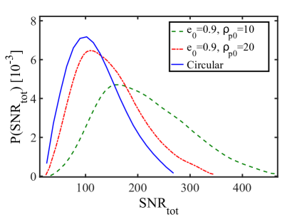
Figure 1 displays the distribution of the for precessing highly eccentric BH binaries detected with the detector network described in Table 1, assuming binary parameters , , , and similar binaries in the circular limit (see Appendix A for details). Generally, similar to the results of O’Leary et al. (2009) (see Figure 11 therein, which corresponds to a single aLIGO detector), the is systematically higher for binaries with than for binaries with . We find that increasing the initial eccentricity from to for fixed does not change the significantly (see Table 3 below), hence we expect that the distribution of for fixed converges in the limit. This is expected since Figure 10 in O’Leary et al. (2009) shows that a low amount of the accumulates near for low to moderately high BH masses.
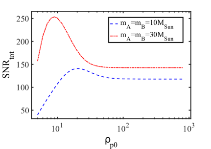
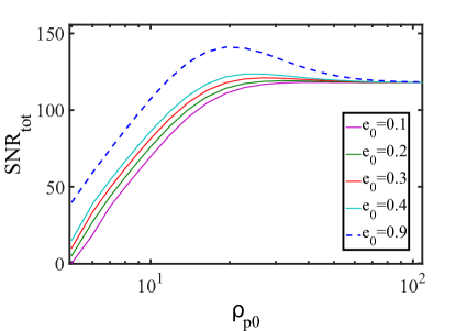
Figure 2 shows that the increases rapidly with for low , has a maximum between and , and decreases for higher approaching the circular binary limit for . These findings may be understood qualitatively as follows. Within the binary forms with a characteristic frequency above in the detector band (see Equation (59) in Gondán et al., 2017). The rapid decrease of the for decreasing is due to the fact that we neglect the GWs of the first hyperbolic encounter (Kocsis et al., 2006b). The decrease of the at high is due to the fact that part of the GW spectrum falls outside of the detectors’ sensitive frequency band. For very large , the binary becomes circular by the time it enters the detectors’ sensitive frequency band, and a significant fraction of the accumulates only in the harmonic (Figure 9), which explains the flat asymptotics for high . Decreasing from high to moderate values higher harmonics start to contribute to the (Figure 9), which explains the increase of the . A combination of these arguments leads to the peak of the at an intermediate value seen in Figure 2. However, note that in addition to neglecting the initial hyperbolic encounter and the final coalescence/ringdown segments of the signal, our waveform model also neglects contributions of spherical moments beyond the quadrupole-order and deviations from a precessing Keplerian orbit (Davis et al., 1972; Berti et al., 2010; Healy et al., 2016). This approximation may not be valid for low (particularly for ). The is expected to be underestimated in this region in Figure 5.
| Circular | Circular | Circular | |||||||
|---|---|---|---|---|---|---|---|---|---|
| quantile | |||||||||
6.2. Parameter measurement errors
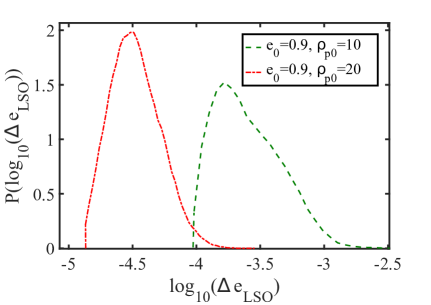
We present the measurement accuracy for the final eccentricity at the LSO for parameters grouped as
| (51) | ||||
| (52) |
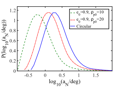
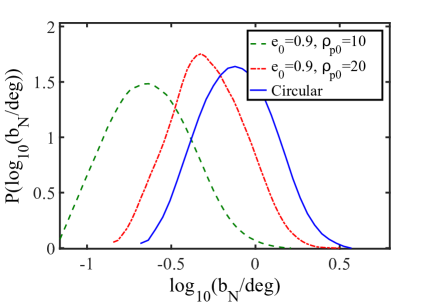
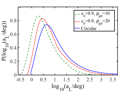
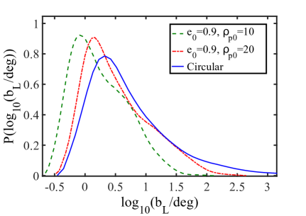
(Kocsis et al., 2007). The fast parameters are related to the high frequency GW phase, while the slow parameters appear only in the slowly-varying amplitude of the GW signal. Slow parameters are mostly determined by a comparison of the GW signals measured by the different detectors in the network. For the polar angles describing the source direction, we calculate the minor and major axes () of the corresponding 2D sky location error ellipse and its area (), and we do the same for the binary orientation error ellipse and its area ().
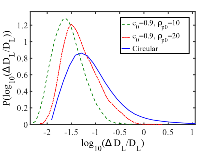
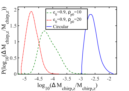
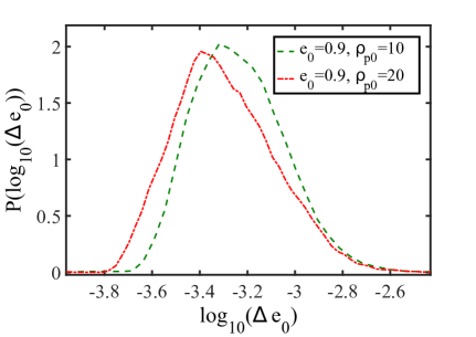
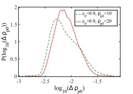
Figures 3 and 4 show the distribution of the measurement errors for randomly chosen source sky position and binary orientation for and , and for the circular limit (see Appendix A), while Table 2 shows the , , and quantiles of the error distributions. Compared to a binary, a binary is more eccentric throughout its evolution, which leads to a higher , and most of its measurement errors are smaller. There are, however, exceptions to this finding: the fast parameters such as the mass parameters and the eccentricity have higher errors for than for (see discussion below).
Many of the binaries in galactic nuclei121212particularly the heavy BHs therein (Gondán et al., 2017) form with very high , close to unity, in single-single encounters due to GW emissions (O’Leary et al., 2009; Gondán et al., 2017). However, similarly to the finding that the does not increase significantly for , we find that parameter errors do not improve due to the early very eccentric evolutionary period beyond (repeated burst phase) compared to waveforms with as shown in Table 3. However, some parameters’ measurement errors improve more significantly with . In particular, the measurement errors of the mass parameters () improve by a factor of , and the measurement error of improves by if increasing from for . This difference is due to the fact that eccentricity modifies the GW phase significantly, which affects the determination of parameters only.
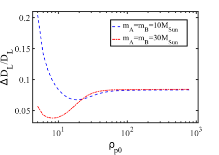
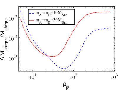
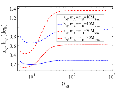
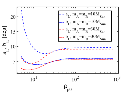
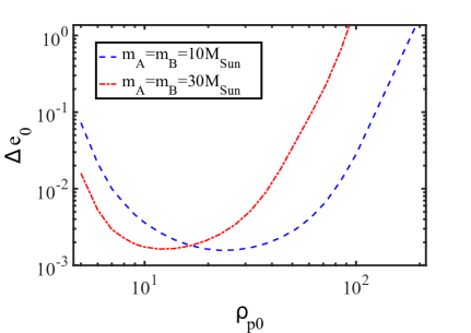
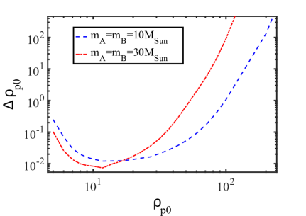
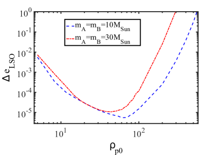
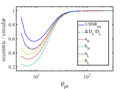
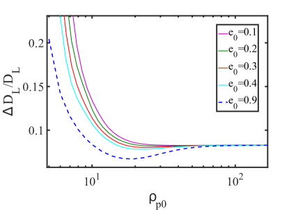
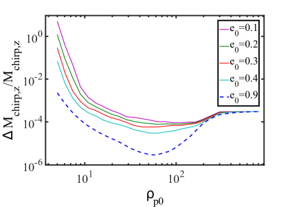
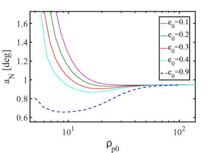
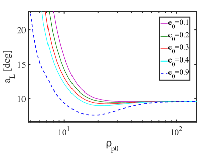
We calculate the parameter measurement errors for precessing highly eccentric BH binaries as a function of for some arbitrarily fixed binary direction and orientations. For one such binary direction and orientation Figure 5 shows the dependence of , , , , , semi-major and semi-minor axes of the sky position error ellipse , and semi-major and semi-minor axes of the error ellipse for the binary orbital plane normal vector direction . Not e that we find similar trends with for other random choices of binary direction and orientation. We find that measurement errors systematically decrease with decreasing for precessing highly eccentric binaries relative to similar binaries in the circular limit (Appendix A), and the errors have a minimum in the range and deteriorate rapidly for . The latter is due to the rapid decrease of the in that range. The dependence of and the principal axes of the sky position and binary orientation error ellipses and (i.e. quantities derived from slow parameters, see Section 5) are qualitatively similar to that of in the complete range of (i.e. they decrease rapidly with for low , have a minimum at moderate , and converge asymptotically to the value of precessing highly eccentric binaries in the circular limit), see Figure 6 for details. However, Figure 5 shows that the chirp mass errors have a minimum at much higher , i.e. between and for and precessing highly eccentric BH binaries, respectively. The main reason for the different behavior of the chirp mass from the distance and angular errors is the fact that the chirp mass is a fast parameter, while the distance and angular parameters are slow parameters. Slow parameters are insensitive to the GW phase perturbations, and depend on the GW amplitude, which is set by the . The SNR of the early part of the waveform near the low-frequency noise wall of the detector is small. However, fast parameters depend sensitively on the GW phase, and the GW phase accumulates mostly at low frequencies, since the residence time (i.e. ) is largest at low orbital frequencies. Thus, the fast parameters’ errors are minimized for binaries which form with with a value for which the GW characteristic frequency is near the detectors’ minimum frequency. The peak of the spectrum is initially at if (Gondán et al., 2017). A slightly lower value of leads to values that represent the minimum of the fast parameters. This also leads to the result observed in Figure 3 that these parameters have higher errors for than for .
In Figure 5, note that errors are relatively small for relatively high up to . At high , the orbital eccentricity approaches zero when it enters the aLIGO band, and increases. We note that the posterior probability distribution function of is well-defined even in the circular limit , and is finite for a given confidence region. However, the Fisher matrix algorithm becomes invalid in this regime as the signal is not approximated well by its linear Taylor expansion with respect to the parameter, since its first derivative vanishes in the circular limit. Therefore the true asymptotic value of for high cannot be recovered with the Fisher matrix technique used in this paper. Further, note that and also increase rapidly with for high . This is due to the fact that for these parameters the binary forms with a pericenter frequency smaller than the minimum frequency of the detector network, and the information on and is limited to higher harmonics with small power. Thus, these parameters indeed have a very high error and become indeterminate in the circular limit. The fact that the relative error of and can be less than percent in the range () for () precessing highly eccentric BH binaries implies that the GW detections might have the potential to constrain the formation environment of these system (O’Leary et al., 2009; Cholis et al., 2016; Rodriguez et al., 2016a, b; Chatterjee et al., 2017; Gondán et al., 2017; Kocsis et al., 2017; Samsing & Ramirez-Ruiz, 2017; Silsbee & Tremaine, 2017).
Furthermore, we found from numerical investigations that does not correlate significantly with other parameters’ errors, which is due to the fact that is measured from the truncation of the signal for at the start of the waveform, while other parameters of a precessing eccentric binary are measured from the inspiral rate (Section 5). However, behaves differently from in this regard, which is due to the fact that is determined by in Equation (5), and depends on the mass parameters.
6.3. Comparison with previous results
In this paper, we have determined the SNR and the expected accuracy with which the aLIGO-AdV-KAGRA detector network may determine the parameters that describe highly eccentric BH binaries, and investigated how these quantities depend on the initial pericenter distance and initial eccentricity . There are some previous studies that also made similar investigations for eccentric compact binaries with significant differences (Yunes et al., 2009; Kyutoku & Seto, 2014; Sun et al., 2015; Ma et al., 2017). They considered different detector networks, applied different waveform models, and used different definitions for and . As a consequence, only a qualitative comparison is possible with those results, which we discuss in this section. At the end of this section, we compare our results for the measurement errors in the circular limit with those presented in previous studies.
We first compare our results with a previous study for the dependence of the . Our result for the dependence of the (Figure 2) is qualitatively in agreement with the result of Figure 2 in Kyutoku & Seto (2014), i.e. the increases rapidly with for low , peaks at a moderate , and converges asymptotically to the value of highly eccentric binaries in the circular limit for high .
In order to compare our results for the dependence of the with Yunes et al. (2009) and Sun et al. (2015), we also set the lower bound of advanced GW detectors’ sensitive frequency band to . We define to be the eccentricity at which the peak GW frequency of the binary defined in Wen (2003) is , and evaluate corresponding to from Equation (37) in Wen (2003) as
| (53) |
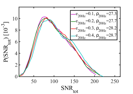
We recalculate the distribution of the for precessing eccentric compact binaries with . The top panel of Figure 7 shows that the is roughly the same for different , which is consistent with results presented in Figure 2 in Sun et al. (2015) and in the left panel of Figure 8 in Yunes et al. (2009). Moreover, we find that the increases weakly with , which is in agreement with results in the left panel of Figure 8 in Yunes et al. (2009). Note that this result disagrees with Table 5 in Sun et al. (2015). The does not depend significantly on in the range of for for as seen in the bottom panel of Figure 7.131313For binaries with relatively high , binaries are well-circularized by the time their peak GW frequency enters the sensitive frequency band of advanced ground-based GW detectors, thus the information about the initial eccentricity vanishes from the detectable part of the waveform. This explains the very weak dependence of the and of parameter measurement errors for high in the bottom panel of Figure 7 and in Figure 8. For binaries with and , we find that is high enough to fall into the range of where the depends on at the level for . The influence of on the increases with since in this case is lower as shown by Equation (53). Thus, the influence of on the distribution of is more significant for higher-mass low-eccentricity binaries. Examples for this characteristic of the are seen in Figure 8 in Yunes et al. (2009).
Finally, we compare our results with previous studies for the dependence of measurement errors of parameters describing eccentric binaries. Sun et al. 2015; Ma et al. 2017 set the initial orbital parameters to be () and (). For various values of () in the range and the corresponding values of (), they determined the measurement accuracies for various parameters of eccentric binaries. Since they applied different waveform models and different parameters describing the eccentric binaries, we resort to a qualitative comparison. We repeated the analysis of Figure 5 for and determined the measurement error of parameters as a function of as shown in Figure 8. We find qualitative agreement with Sun et al. (2015); Ma et al. (2017). The measurement accuracies of parameters increase strictly monotonically with .
Previous papers have investigated the dependency of the measurement errors for by using different PN order waveform models for non-spinning inspiraling binaries for a fixed SNR in a single aLIGO type detector. Previous results showed that the measurement accuracy of these parameters decreases with increasing for provided that the SNR accumulated in one GW detector is fixed, see Table 1 in Arun et al. (2005) and references therein. Therefore, we determined the measurement errors in the circular limit for for a qualitative comparison.141414A quantitative agreement is not expected since our precessing waveform model differs from the waveform models in those studies. To calculate the measurement error of the parameter we use the fact that and so
| (54) |
In agreement with the 1PN order case in Arun et al. (2005), we find that , , , and increase with for fixed (Table 4). Such a qualitative agreement is expected since the adopted precessing eccentric waveform approximates the full 1PN waveform in its most important features, and the -dependent trends of error distributions do not depend on the number of detectors or on the sky position or angular momentum unit vectors of the source.
7. Summary and Conclusion
We carried out a Fisher-matrix-type study to determine the accuracy with which the parameters of highly eccentric BH binaries may be measured using the aLIGO-AdV-KAGRA GW detector network. Eccentricity changes the GWs of binaries compared to circular binaries, in several ways. In time-domain, the gravitational waveform of eccentric binaries is quasiperiodic but not sinusoidal. Relativistic precession adds a slow amplitude modulation to the waveform for each polarization. Eccentricity also changes the inspiral rate at which the binary separation and period shrink. We take all of these effects into account using the stationary phase approximation (Moreno-Garrido et al., 1994; Mikóczi et al., 2012). In contrast to circular binaries, the waveform of eccentric binaries includes several prominent orbital frequency harmonics, general relativistic precession causes each harmonic to split into three frequencies for both GW polarizations respectively, and the eccentric inspiral creates a spectrum, which is different from the waveform of circular inspiral sources for each harmonic. These features in the waveform make it possible to accurately determine the eccentricity and angle of periapsis, and the modulated inspiral rate improves the measurement accuracy of mass parameters for eccentric inspirals.
The main parameters that describe eccentric inspiraling binaries are the initial pericenter distance when the eccentricity is close to unity and the final eccentricity at the last stable orbit . These parameters are systematically different for different formation channels. Thus their measurement may have important implications on the astrophysical origin of the sources (O’Leary et al., 2009; Cholis et al., 2016; Rodriguez et al., 2016a, b; Chatterjee et al., 2017; Gondán et al., 2017; Samsing & Ramirez-Ruiz, 2017; Silsbee & Tremaine, 2017). Based on a survey with and precessing highly eccentric BH binaries at using the planned aLIGO-AdV-KAGRA detector network, our results are be summarized as follows.
-
1.
The improves by a factor of (depending on , the component masses, and the sky position and binary orientation angles, see Figure 1) for precessing highly eccentric BH binaries compared to similar binaries in the circular limit 151515We adopted the leading order stationary phase approximation waveform for circular sources. with the same masses and distance. The volume in the Universe for a fixed maximum is () larger for eccentric inspiraling binaries with () than for similar binaries in the circular limit.
-
2.
We determined how the parameters’ measurement accuracies depend on the initial dimensionless pericenter distance () for precessing highly eccentric BH binaries. The smallest errors are obtained for small values for the sky position and angular momentum and for the luminosity distance and . However, the errors for fast parameters, which are sensitive to the GW phase, like the chirp mass, the initial eccentricity, and the eccentricity at the last stable orbit improve most significantly for a higher between and (Figure 5).
-
3.
The parameter estimation errors can improve significantly for highly eccentric precessing BH binaries compared to similar binaries in the circular limit by a factor of (depending on , the component masses, and the sky position and binary orientation angles, see Figures 3 and 5)
-
•
for the mass errors,
-
•
for the semi-major and semi-minor axes of the sky localization ellipse,
-
•
for the distance errors,
-
•
for the semi-major and semi-minor axes of the error ellipse for the binary orientation.
-
•
-
4.
For initially highly eccentric BH binaries at , the measurement errors for parameters specific to precessing highly eccentric BH binary sources may be as low as of order (depending on , the component masses, and the sky position and binary orientation angles, see Figures 4 and 5)
-
•
for the final eccentricity errors at LSO,
-
•
for the initial eccentricity errors,
-
•
for the initial pericenter distance.
-
•
For initially moderately eccentric to low eccentricity binaries, the parameter measurement errors and SNRs improve by a smaller amount for low to intermediate (Figure 8).
Note that the eccentricity errors are remarkably low, which is not surprising given that eccentricity is encoded in several measurable features of the waveform including the orbital harmonics, the splitting of each frequency harmonic into triplets, the frequency evolution of harmonics (the “chirp”), the frequency evolution of the distance between the spectral triplets, the low frequency cutoff of the signal at the initial pericenter frequency, and the eccentricity dependence of the last stable orbit where the inspiral transitions into a rapid coalescence.
However, there are several factors which may significantly increase the measurement errors in more typical cases. First, more typical sources are expected to be at much larger distances than . Assuming crudely that the eccentricity errors scale with , the median measurement errors for a precessing highly eccentric BH binary at (similar to GW150914) are expected to be () for the final eccentricity at the last stable orbit if () for the design sensitivity of the aLIGO/AdV/KAGRA instruments. In these cases, the expected median initial eccentricity error is , and the median initial pericenter distance is (; see Table 2).
Another important simplifying assumption, which may have skewed the errors to lower values, was to neglect higher order post-Newtonian (PN) corrections which depend on the spin of the merging objects. The spins of the two binary components introduce additional parameters, which may become partially degenerate with all other parameters thereby increasing their errors. On the other hand, spin precession breaks degeneracies between the binary orientation and other slow parameters (Lang & Hughes, 2006; Kocsis et al., 2007; Chatziioannou et al., 2014). However, the eccentricity-induced orbital harmonics enter at the Newtonian order, the frequency-triplets due to GR precession enter at the low PN order. Therefore, the eccentricity-related spectral features are dominant already at the early stages of the inspiral when higher order PN corrections are negligible. For this reason, the estimated and errors are expected to be robust. On the other hand, most of the SNR accumulates at late times for stellar-mass BH binaries where the high order PN corrections are significant. We leave an estimate of parameter estimation errors for spinning binaries to future work.
Finally, an important simplification is the Fisher matrix method itself, which is valid only if the waveform model is a faithful representation of the GW signal and the noise is Gaussian and sufficiently small that the SNR is sufficiently large that the parameter error region is an ellipsoid in parameter space and when the parameter derivate of the waveform is non-vanishing. For smaller SNR, the parameter error region geometry is more complex and the uncertainties are generally higher (see Cornish & Littenberg, 2015, and reference therein). The parameter estimation errors may also be affected by theoretical uncertainties of the waveform model (Cutler & Vallisneri, 2007), which may be especially important for highly eccentric binaries, where the post-Newtonian expansion is slowly convergent (Kocsis & Levin, 2012).
Such low eccentricity errors may give the aLIGO-AdV-KAGRA GW detector network the capability to distinguish among different astrophysical formation channels. In a companion study (Gondán et al., 2017), we illustrate the expected distribution of eccentricities and other physical parameters for single-single GW capture sources in galactic nuclei. Similar studies for other astrophysical formation channels are underway.
Future multi-waveband searches of eccentric inspiral sources with LISA and aLIGO-AdV-KAGRA (Kocsis & Levin, 2012; Sesana, 2016) have good prospects for even more accurate measurements of the physical parameters well beyond the level reported here. In that case the GW frequency range is much wider. Since eccentricity decreases due to GW emission, eccentricity may be expected to be much higher at lower frequencies in the LISA band. This leads to a much larger total GW phase shift caused by eccentricity. The better measurement of relativistic precession may more efficiently break degeneracies between mass and other parameters. The modulation caused by the orbit of the instrument around the Sun and Earth’s spin can help break degeneracies among source direction, orientation, and other parameters. Accounting for eccentricity for third generation Earth based (e.g. Einstein telescope), deci-Hertz to mHz space-based instruments will be essential (Chen & Amaro-Seoane, 2017).
Acknowledgment
We thank the anonymous referee for constructive comments, which helped improve the quality of the paper. This project has received funding from the European Research Council (ERC) under the European Union’s Horizon 2020 research and innovation programme under grant agreement No 638435 (GalNUC) and by the Hungarian National Research, Development, and Innovation Office grant NKFIH KH-125675. This work was performed in part at the Aspen Center for Physics, which is supported by National Science Foundation grant PHY-1607761. The calculations were carried out on the NIIF HPC cluster at the University of Debrecen, Hungary.
Appendix A The circular limit
The circular limit follows from the limit for arbitrary or for arbitrary (see Figure 5 in O’Leary et al. (2009)). In practice we set , , and omit the parameters from the Fisher matrix that become degenerate or unconstrained in the circular limit: , , and . Thus, the parameters in the circular limit are
| (A1) |
where arises due to precession even in the circular limit (see Equation (25)). In the limit, and , however the Fisher matrix algorithm becomes invalid for in this limit (Section 6.2).
We have also examined how the measurement errors depend on the total mass of the binary in the circular limit, and qualitatively compared our results to those of previous parameter estimation studies in Section 6.3. We have found an excellent match between our results and the results of previous studies.
Appendix B Response of an individual ground-based detector
Here we describe the measured signal of individual ground-based detectors, and introduce the adopted coordinate system.
We define the Cartesian coordinate system with basis vectors , , and a spherical coordinate system () fixed relative to the center of the Earth, such that and is along the North geographic pole and is along the prime meridian. We denote the unit vector pointing from the center of Earth to the binary’s sky position as , and define to be the normal vector parallel with the binary’s orbital angular momentum,
| (B1) | ||||
| (B2) |
We denote the unit vectors parallel with the arms of the -th detector as and , and set . As and are parallel with the surface of Earth for all detectors, points from the center of Earth toward the geographical location of the detector. Let the coordinates () denote the location of the detector, thus the unit vectors along the arms can be expressed as
| (B3) |
| (B4) |
| (B5) |
(Creighton & Anderson, 2011), where the orientation angle of the detector, , is defined in Section 3.
These vectors define the response tensor for the detector:
| (B6) |
(Finn & Chernoff, 1993), where and are the Cartesian components of and .
We adopt the basis vectors following the conventions of previous studies (Finn & Chernoff, 1993; Cutler & Flanagan, 1994; Anderson et al., 2001; Dalal et al., 2006; Nissanke et al., 2010)
| (B7) |
with preferred polarization basis tensors
| (B8) | |||
| (B9) |
where and are Cartesian components. Thus, the transverse-traceless metric perturbation describing the GW is written as
| (B10) |
The response of the detector to a GW with frequency can be given in time-domain by
| (B11) |
(Nissanke et al., 2010), where is the position of the detector, the factor measures the light travel time between the detector and the coordinate origin, thus the factor measures the phase shift between the detector and the coordinate origin. In Equation (B11), and are the antenna factors
| (B12) |
In our calculations, Earth is taken to be a sphere with radius of .
If the time that the GW signal spends in the detectors’ sensitive frequency band is negligible compared to the rotation period of Earth, then the measured waveform in frequency domain for the detector is
| (B13) |
where and are the Fourier-transformed expressions of and at Earth’s center, and and are given by the (practically time-independent) orientation of the detectors shown in Table 1.
Similarly, using the frequency harmonic triplets for eccentric precessing inspiraling binaries in the stationary phase approximation, the measured waveform for the detector is
| (B14) |
where and can be derived from and by multiplying each term of with the phase shift factors and for each harmonic, respectively. More specifically, the measured signal’s Fourier phase in Equations (35) and (36) in the detector is shifted respectively according to
| (B15) | ||||
| (B16) |
Appendix C Time evolution of the orbit
In this section, we derive the time evolution of different harmonics in the detectors’ sensitive frequency band, and for each orbital harmonic we determine the eccentricity at which the signal enters the detectors’ sensitive frequency band. These formulae will be utilized in Appendix D.
The time-dependent GW signal of a precessing eccentric BH binary as measured by the detector can be given as
| (C1) |
where and are given in Equations (2.1) and (2), and and are quantified by Equation (B12). We neglect spins in this study, therefore the angular momentum vector direction is conserved during the eccentric inspiral (Cutler & Flanagan, 1994). The polar angle of the source relative to the detector depends on the rotation phase of Earth during the day. We neglect Earth’s rotation, since the total duration of an eccentric inspiral from to merger is of order as shown in Figure 3 in O’Leary et al. (2009). 161616Earth’s rotation may be relevant for highly eccentric low mass compact objects with large , such as neutron star binaries. For black holes, if , then the signal mostly circularizes before it enters the detectors’ sensitive frequency band, and the amount of time it spends in the band with a significant is limited to less than a minute. For an illustration of the accumulation of the with time we refer the reader to Figure 10 of O’Leary et al. (2009) and Figure 7 of Kocsis & Levin (2012).
The waveform of an eccentric binary in the stationary phase approximation is a sum over harmonics for each component of the frequency triplet () with different reference times (see Section 2.2). During the evolution (and ) shrinks strictly monotonically in time (Peters, 1964), therefore its inverse function is well-defined and determines , , and . For inspiraling circular binaries, time can be expressed using the frequency of the emitted GW signal as
| (C2) |
(see equations (2.13) and (2.19) in Cutler & Flanagan (1994) for details), where the constant of integration, , is defined by the requirement that as . We generalize Equation (C2) for eccentric inspirals by changing the integration variable from to in Equation (C2),
| (C3) |
where is given by Equation (15), and we introduced
| (C4) |
and substituted using Equation (22). Here and are given by Equations (21) and (19), and in Equation (C3) is of form
| (C5) |
(see Mikóczi et al., 2012, for an analytic result). Using Equation (C3) we get the total duration of the harmonic in the detector’s sensitive frequency band
| (C6) | ||||
| (C7) | ||||
| (C8) |
Here () refers to the eccentricity at which the harmonic () reaches the LSO or when it exists the detectable highest frequency for the given detector, and () refers to the eccentricity at which the signal related to () first enters the detector’s sensitive frequency band or when it forms within the band. Thus,
| (C9) | ||||
| (C10) |
where
| (C11) | ||||
| (C12) | ||||
| (C13) |
Here is given analytically by Equation (18), denotes the inverse function of , and are the lower and upper limits of the detector’s sensitive frequency band (typically and , respectively), and is determined by Equation (21). Similarly, we define the parameters corresponding to and as
| (C14) | ||||
| (C15) | ||||
| (C16) | ||||
| (C17) |
where
| (C18) | ||||
| (C19) | ||||
| (C20) | ||||
| (C21) | ||||
| (C22) |
where is given by Equation (25), and is the inverse function of given by Equation (C22).
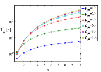
In practice, the second term is negligible in Equations (C6)-(C8). We find that and are within of for any fixed . The top panel of Figure 9 shows the total time the GW signal spends in an aLIGO type detector’s sensitive frequency band for different harmonics. Higher harmonics enter the aLIGO band earlier and that depending on the first 10 orbital harmonics spend between seconds to minutes in the detector’s sensitive frequency band for a precessing highly eccentric BH binary.
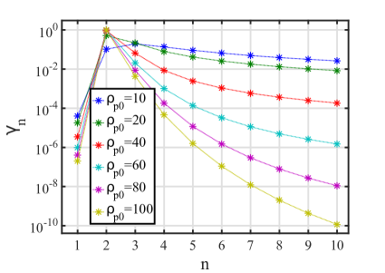
The bottom panel of Figure 9 shows the fraction of the squared SNR that accumulates in different orbital harmonics for various for aLIGO. For high , the signal effectively circularizes by the time it enters the detector’s sensitive frequency band and the harmonic dominates. However, the contribution of is significant for for a precessing highly eccentric BH binary.
Appendix D Calculating the signal-to-noise Ratio and the Fisher matrix
In this section, we derive numerically efficient formulae to calculate the SNR and the Fisher matrix for individual detectors. We first neglect pericenter precession, then extend the calculations for precessing eccentric sources.
D.1. Signal-to-noise ratio
D.1.1 Eccentric inspirals without precession
The NoPrec signal measured by a detector at position is given in Fourier space from Equations (2.2) and (2.2) as
| (D1) |
where is the Fourier phase at the origin of the coordinate system set to the Earth’s center, given by Equation (35), we set , , denotes the Heaviside function, which is zero and unity for negative and positive arguments171717More precisely, we assume a smoothed truncation of the signal as (D2) where is the absolute change of the eccentricity during the first orbit, which from Equations (14) and (15) is (D3) where ., respectively, and
| (D4) |
where and are given by Equations (33) and (34), and are given by Equations (5) and (7), specifies the argument of pericenter, which is assumed to be fixed here, and are the antenna factors given by Equation (B12). The factor gives the phase shift of the measured signal between the position of the detector and the origin of the coordinate system for the harmonic (Appendix B). depends on implicitly through and .
In Equation (D1), accounts for the start of the waveform when the binary forms with initial eccentricity181818The initial eccentricity does not enter the waveform anywhere else, and are independent of . Due to this term, and may be measured independently, and follows from Equation (5). . Along the same lines, a similar term could be incorporated to account for the end of the eccentric inspiral where the waveform transitions to a plunge and ringdown phase. However, we conservatively do not account for such a term, since the waveform near the end of the inspiral is sensitive to higher order post-Newtonian corrections, which are not known and neglected here (Kocsis & Levin, 2012; Loutrel & Yunes, 2017). Nevertheless, the inspiral rate is sensitive to in Equations (18) and (19) and (22), which affects and .
For each detector, the square of the SNR for the NoPrec waveform, , can be obtained by substituting into Equation (42). We find that the product of sums in is dominated by the elements such that 191919Numerically we confirm that cross-terms proportional to have a negligible contribution for .
| (D5) |
where is the frequency at which the harmonic first enters the detector’s sensitive frequency band or when it forms in the band, and similarly is the frequency at which the signal exits the detector’s sensitive frequency band or when it reaches the LSO,
| (D6) | ||||
| (D7) |
Computationally it is practical to change the integration variable from to as
| (D8) |
thus Equation (D5) can be rewritten generally as
| (D9) |
where is given analytically by Equation (18), and may be obtained from Equation (D.1.1) by substituting . The integration bounds and are given by Equations (C9) and (C10). We truncate the calculation beyond a maximum spectral harmonic defined in Equation (37).
accurately recovers Equation (D5) generally for any value of the initial eccentricity in the range , however the number of considered harmonics increases rapidly for high (Equation 37), and in the limit . Therefore, is computationally efficient for low to moderate initial eccentricities () and it is inefficient for higher . In order to make computationally efficient for high initial eccentricities, we reverse the order of the sum and the integral in Equation (D9) and truncate the sum over harmonics at (O’Leary et al., 2009).202020In this case the number of considered harmonics reduces significantly. Thus, we get
| (D10) |
We use the above introduced trick to derive computationally efficient formulae in the high initial eccentricity limit for Fisher matrix elements in the precession-free case (Appendix D.2.1) and for the SNR and the Fisher matrix elements in the precessing case (Appendices D.1.2 and D.2.2).
D.1.2 Eccentric inspirals with precession
We derive the SNR of the precessing model in this section. The Fourier-transformed waveform given by Equation (B14) can be rewritten as
| (D11) |
where the terms , , and are defined as
| (D12) | ||||
| (D13) | ||||
| (D14) |
The terms and depend on through , which are expressed with using Equations (29) and (30). Furthermore these equations depend on and through and (e.g. and ).
Next, we substitute this waveform into Equation (42). Similarly to that of the NoPrec signal (Equation D1), cross terms in the product of sums in have negligible contributions to , and so
| (D15) |
where and are defined in Equations (D6) and (D7). The integration bounds for the integrals over are defined similarly to and in Equation (D6) and (D7),
| (D16) | ||||
| (D17) |
where is defined in Equation (C22).
Next, we change integration variables from to using Equation (D8) and similarly from to using Equation (30) as
| (D18) |
Here is given by Equation (25) as
| (D19) |
After truncating the sum over the harmonics to the relevant range as in Equation (D9), Equation (D.1.2) can be written as
| (D20) |
where and . The integration bounds are given by Equations (C14) and (C17).
Similarly to , is computationally efficient only for low to moderate initial eccentricities (). For high initial eccentricities, the computationally efficient form of , , can be given by reversing the order of the sum and the integral as
| (D21) |
D.2. Fisher Matrix
Due to the similarity of the equations defining the SNR (see Equation (42)) and the Fisher matrix (see Equation (44)), we may follow the same procedure to derive numerically efficient formulae for the Fisher matrix in the limit of high initial eccentricity. Similarly to Appendix D.1, we start the analysis with the NoPrec model and then generalize the calculation to the Prec model, which accounts for the precessing case.
D.2.1 Eccentric inspirals without precession
Let us substitute Equation (D1) into Equation (44). Similarly to the product of sums of orbital harmonics , we find numerically that the cross-terms in with have a negligible contribution to . Thus, we find that the stationary phase approximation is applicable if we drop the cross-terms, and thus in Equation (44) we may use
| (D22) |
Here
| (D23) |
and
| (D24) |
where
| (D25) |
and and are given by Equations (D.1.1) and (35). We first differentiate the expressions in the bracket in Equation (D24) with respect to , then change the variable from back to . Note that for all and , is independent of , and so for . In Equation (D.2.1), in the second, third, and fourth terms denote the Kronecker-, defined to be unity if and zero otherwise. In Equation (D.2.1), the second and third terms arise due to the Heaviside function in the waveform in Equation (D1), which represents the start of the waveform with eccentricity . The -derivative of this function is , which denotes the Dirac- function. Note that we use a smoothed version of over a scale , which is given in Equation (D2), whose derivative is approximately212121We neglect the partial derivatives of with respect to the physical parameters.
| (D26) |
To avoid confusion note that the numerator denotes the Dirac- function, which has a unit integral over , and in the denominator is the quantity given by Equation (D3).
Furthermore, we note that
| (D27) |
in Equation (D.2.1). In these equations enters when substituting for . By substituting Equation (D.2.1) into Equation (44), changing the integration variable from to respectively for each harmonic using222222Note that depends on as seen in Equations (18) and (22). and Equations (18) and (22), and truncating the sum over the harmonics to the relevant range, the Fisher matrix becomes232323We label this general expression with “Gen” to distinguish from an approximation “High” used below for high eccentricities.
| (D28) |
The limits of integration in Equation (D.2.1) are defined by Equations (C9) and (C10). Here the four terms correspond respectively to the four terms in Equation (D.2.1). The first term is directly analogous to that appearing in the SNR (see Equation D10). Note that in particular, the elements corresponding to and terms are nonzero. The -dependence enters in as shown in Equations (18) and (22). However, the first term in Equation (D.2.1) is zero for the and elements. If the binary forms in the detector’s sensitive frequency band the second, the third, and the fourth terms in Equation (D.2.1) contribute to this element of the Fisher matrix. The eccentricity integral in the Fisher matrix may be carried analytically over the function, which yields the second and third terms in Equation (D.2.1). There is the Kronecker-, which is zero unless corresponds to the parameter , and similarly for . Note further that only harmonics with contribute to these boundary terms, since otherwise .
Similarly to the , is generally valid for any initial eccentricity in the range , but it is computationally efficient only for low to moderate initial eccentricities (). In order to make the calculation computationally efficient for high initial eccentricities, we reverse the order of the sum and the integral in the first term in Equation (D.2.1), and truncate the sum over harmonics at as in Appendix D.1.1. We get
| (D29) |
D.2.2 Eccentric inspirals with precession
Following the steps of Appendix D.2.1 for the precession-free model, we may generalize the calculation of the Fisher matrix to include precession similar to Appendix D.1.2. The Fisher matrix, which is computationally efficient for low to moderate initial eccentricities (), can be given as
| (D30) |
where
| (D31) |
and
| (D32) |
where the integration bounds are given by Equations (C14)-(C17), and
| (D33) | ||||
| (D34) |
Similar to the precession-free case, here
| (D35) | ||||
| (D36) |
where and are given by Equations (D12)-(D.1.2), and are expressed by Equations (35) and (36), and we first differentiate the expressions in the bracket in Equations (D33) and (D34) with respect to , then change variables from and back to . Similar to the precession-free case, only harmonics with and contribute to the boundary terms in Equations (D.2.2) and (D.2.2), since otherwise and .
For high initial eccentricities, the computationally efficient form of , , can be derived by reversing the order of the sum and the integral in the first term in Equations (D.2.2) and (D.2.2), and truncating the sum over harmonics at as in Appendix D.1.1. Thus, can be given as
| (D37) |
where
| (D38) |
and
| (D39) |
Appendix E Validation of Codes
E.1. Analytic circular limit without precession
First, we study the circular limit of the eccentric waveform, and , defined by Equations (2.2) and (2.2) for the NoPrec model. For , and implying that is degenerate with , which we henceforth omit. After integrating the term over in Equation (26) according to previous considerations, substituting with , and expanding the expression of , the polarization components become
| (E1) | ||||
| (E2) |
where the phase function can be given as
| (E3) |
These are indeed the well-known frequency domain polarization components of circular binaries in leading order (Cutler & Flanagan, 1994). The parameter set characterizing this waveform is
| (E4) |
For validation tests, we calculate the SNR of circular binaries, , for a single aLIGO detector. is calculated by substituting Equations (E1) and (E2) into Equation (B13) and then using Equation (42). The Fisher matrix of circular binaries for the parameter set for each detector is calculated by substituting Equations (E1) and (E2) into Equation (B13) and then using Equations (44).
E.2. Eccentric inspiral without pericenter precession
Next, we discuss validation tests performed for the codes using the NoPrec waveform model. In this case, the parameters are
| (E5) |
Compared to , includes (set by and , see Equation (22)) and .
E.2.1 Signal-to-noise ratio
First, we generate a set of source parameters for comparison , and compare the output of with the output of in the circular limit for a single aLIGO detector (Table 1). Here and in further validation test, the set of fiducial source parameters generated for comparison are , where and are drawn from a uniform distribution between , the set of and are drawn from a uniform distribution between , and are drawn from a uniform distribution between , and is drawn from a uniform distribution between . The generation of other source parameters are described in details in the corresponding paragraph. We assume the fiducial value for each binary, and in practice we set and when considering the circular limit (Appendix A). We find that the relative discrepancy between and is less than in all cases.
Next, we examine if the output of agrees with Figure 11 in O’Leary et al. (2009), which shows the source sky position- and orientation-averaged RMS SNR for a single aLIGO detector as a function of and . O’Leary et al. (2009) used the Fourier domain orbit-averaged leading order waveform (Peters & Mathews, 1963), which corresponds to our NoPrec model. We set the sensitivity curve to that used in O’Leary et al. (2009), set , and find the results for several and in the range and of , respectively. For each and , we generate random Monte Carlo samples of source sky location () and binary orientation () as introduced above in this section. We find that the RMS of the distributions are in agreement with the results of Figure 11 in O’Leary et al. (2009).
Finally, we generate a set of source parameters for comparison, and compare the output of and for several high and and for a single aLIGO detector. In particular, and are drawn from a uniform distribution between and in these calculations, respectively. The relative discrepancy between and is less than in all cases.
E.2.2 Fisher matrix
Since the parameter set of the leading order circular and eccentric binaries, and differ, see Equations (E4) and (E5), we cannot simply compare the output of with the output of in the circular limit. Therefore, we first restrict to the parameters set . Next, we generate a set of source parameters for comparison, and compare the output of with the output of in the circular limit for the Fisher matrix elements corresponding to the circular parameters and for a single aLIGO detector. The relative discrepancy between and is less than in all cases.
Finally, we generate a set of source parameters for comparison, and compare the output of and for the Fisher matrix elements corresponding to the parameter set in the high eccentricity limit for several and for a single aLIGO detector. Similarly to Appendix E.2.1, and are drawn from a uniform distribution between and in these calculations, respectively. The relative discrepancy between Fisher matrix elements is less than in all cases.
E.3. Eccentric pericenter-precessing binary waveforms
E.3.1 Signal-to-noise ratio
We test the numerical accuracy of the precessing waveform using the following theorem for leading order post-Newtonian binary inspirals. The amount of energy radiated in GWs is equal to the loss of mechanical energy of the binary, which is the same for the NoPrec and for the Prec models. This is due to the fact that determines the mechanical energy of the binary in the Newtonian approximation, and the orbital elements and are not affected by pericenter precession. This also implies that the amount of SNR must be equal for the NoPrec and our precessing models for white noise.
Thus, assuming white noise, we generate a set of source parameters, and compare the output of with the output of for several and , where and are drawn from a uniform distribution between and in these calculations, respectively. The relative discrepancy between and is less than in all cases.
Furthermore, we repeat the same analysis for and , where is drawn from a uniform distribution between . We find that the discrepancy between SNR values is less than in all cases.
Finally, we generate a set of source parameters for comparison, and compare the output of with the output of for several high and and assuming white noise. Similarly to the NoPrec model, and are drawn from a uniform distribution between and in these calculations, respectively. We find that the relative discrepancy between and is less than in all cases.
E.3.2 Fisher matrix
can be validated by following the procedure for , but considering and high values (). We find that the relative discrepancy between Fisher matrix elements are less than in all cases.
Finally, after generating a set of source parameters for comparison, we compare the output of and for the Fisher matrix elements corresponding to the parameter set in the high eccentricity limit for several in the range and for a single aLIGO detector. The discrepancy between Fisher matrix elements is less than in all cases.
References
- Aarseth (2012) Aarseth, S. J. 2012, MNRAS, 422, 841
- Aasi et al. (2012) Aasi, J., Abadie, J., Abbott, B. P., et al. 2012, Classical and Quantum Gravity, 29, 155002
- Aasi et al. (2015) —. 2015, Classical and Quantum Gravity, 32, 115012
- Abadie et al. (2010) Abadie, J., Abbott, B. P., Abbott, R., et al. 2010, Classical and Quantum Gravity, 27, 173001
- Abbott et al. (2016a) Abbott, B. P., Abbott, R., Abbott, T. D., et al. 2016a, ApJ, 818, L22
- Abbott et al. (2016b) —. 2016b, Physical Review X, 6, 041015
- Abbott et al. (2016c) —. 2016c, Physical Review Letters, 116, 241103
- Abbott et al. (2016d) —. 2016d, Physical Review Letters, 116, 061102
- Abbott et al. (2016e) —. 2016e, Physical Review Letters, 116, 241102
- Abbott et al. (2016f) —. 2016f, Living Reviews in Relativity, 19, 1
- Abbott et al. (2016g) —. 2016g, Physical Review Letters, 116, 221101
- Abbott et al. (2016h) —. 2016h, ApJ, 833, L1
- Abbott et al. (2016i) —. 2016i, ApJ, 832, L21
- Abbott et al. (2017a) —. 2017a, Physical Review Letters, 118, 221101
- Abbott et al. (2017b) —. 2017b, ApJ, 851, L35
- Abbott et al. (2017c) —. 2017c, Physical Review Letters, 119, 141101
- Abbott et al. (2017d) —. 2017d, Physical Review Letters, 119, 161101
- Abbott et al. (2017e) —. 2017e, ApJ, 850, L40
- Acernese et al. (2015) Acernese, F., Agathos, M., Agatsuma, K., et al. 2015, Classical and Quantum Gravity, 32, 024001
- Amaro-Seoane & Chen (2016) Amaro-Seoane, P., & Chen, X. 2016, MNRAS, 458, 3075
- Anderson et al. (2001) Anderson, W. G., Brady, P. R., Creighton, J. D., & Flanagan, É. É. 2001, Phys. Rev. D, 63, 042003
- Antognini et al. (2014) Antognini, J. M., Shappee, B. J., Thompson, T. A., & Amaro-Seoane, P. 2014, MNRAS, 439, 1079
- Antonini et al. (2016) Antonini, F., Chatterjee, S., Rodriguez, C. L., et al. 2016, ApJ, 816, 65
- Antonini et al. (2014) Antonini, F., Murray, N., & Mikkola, S. 2014, ApJ, 781, 45
- Antonini & Perets (2012) Antonini, F., & Perets, H. B. 2012, ApJ, 757, 27
- Antonini & Rasio (2016) Antonini, F., & Rasio, F. A. 2016, ApJ, 831, 187
- Arun et al. (2005) Arun, K. G., Iyer, B. R., Sathyaprakash, B. S., & Sundararajan, P. A. 2005, Phys. Rev. D, 71, 084008
- Aso et al. (2013) Aso, Y., Michimura, Y., Somiya, K., et al. 2013, Phys. Rev. D, 88, 043007
- Balser & Wagner (1960) Balser, M., & Wagner, C. A. 1960, Nature, 188, 638
- Barack & Cutler (2004) Barack, L., & Cutler, C. 2004, Phys. Rev. D, 69, 082005
- Bartos et al. (2017) Bartos, I., Kocsis, B., Haiman, Z., & Márka, S. 2017, ApJ, 835, 165
- Belczynski et al. (2016) Belczynski, K., Repetto, S., Holz, D. E., et al. 2016, ApJ, 819, 108
- Berry et al. (2015) Berry, C. P. L., Mandel, I., Middleton, H., et al. 2015, ApJ, 804, 114
- Berti et al. (2010) Berti, E., Cardoso, V., Hinderer, T., et al. 2010, Phys. Rev. D, 81, 104048
- Biswas et al. (2013) Biswas, R., Blackburn, L., Cao, J., et al. 2013, Phys. Rev. D, 88, 062003
- Blackburn et al. (2008) Blackburn, L., Cadonati, L., Caride, S., et al. 2008, Classical and Quantum Gravity, 25, 184004
- Boetzel et al. (2017) Boetzel, Y., Susobhanan, A., Gopakumar, A., Klein, A., & Jetzer, P. 2017, Phys. Rev. D, 96, 044011
- Bose et al. (2016) Bose, S., Hall, B., Mazumder, N., et al. 2016, in Journal of Physics Conference Series, Vol. 716, Journal of Physics Conference Series, 012007
- Breivik et al. (2016) Breivik, K., Rodriguez, C. L., Larson, S. L., Kalogera, V., & Rasio, F. A. 2016, ApJ, 830, L18
- Canizares et al. (2015) Canizares, P., Field, S. E., Gair, J., et al. 2015, Physical Review Letters, 114, 071104
- Cannon et al. (2012) Cannon, K., Cariou, R., Chapman, A., et al. 2012, ApJ, 748, 136
- Cao & Han (2017) Cao, Z., & Han, W.-B. 2017, Phys. Rev. D, 96, 044028
- Chatterjee et al. (2017) Chatterjee, S., Rodriguez, C. L., Kalogera, V., & Rasio, F. A. 2017, ApJ, 836, L26
- Chatziioannou et al. (2014) Chatziioannou, K., Cornish, N., Klein, A., & Yunes, N. 2014, Phys. Rev. D, 89, 104023
- Chen & Amaro-Seoane (2017) Chen, X., & Amaro-Seoane, P. 2017, ApJ, 842, L2
- Cholis et al. (2016) Cholis, I., Kovetz, E. D., Ali-Haïmoud, Y., et al. 2016, Phys. Rev. D, 94, 084013
- Cornish & Key (2010) Cornish, N. J., & Key, J. S. 2010, Phys. Rev. D, 82, 044028
- Cornish & Littenberg (2015) Cornish, N. J., & Littenberg, T. B. 2015, Classical and Quantum Gravity, 32, 135012
- Coughlin et al. (2015) Coughlin, M., Meyers, P., Thrane, E., Luo, J., & Christensen, N. 2015, Phys. Rev. D, 91, 063004
- Creighton & Anderson (2011) Creighton, J., & Anderson, W. 2011, Gravitational-Wave Physics and Astronomy: An Introduction to Theory, Experiment and Data Analysis.
- Csizmadia et al. (2012) Csizmadia, P., Debreczeni, G., Rácz, I., & Vasúth, M. 2012, Classical and Quantum Gravity, 29, 245002
- Cutler & Flanagan (1994) Cutler, C., & Flanagan, É. E. 1994, Phys. Rev. D, 49, 2658
- Cutler et al. (1994) Cutler, C., Kennefick, D., & Poisson, E. 1994, Phys. Rev. D, 50, 3816
- Cutler & Vallisneri (2007) Cutler, C., & Vallisneri, M. 2007, Phys. Rev. D, 76, 104018
- Dalal et al. (2006) Dalal, N., Holz, D. E., Hughes, S. A., & Jain, B. 2006, Phys. Rev. D, 74, 063006
- Damour et al. (2004) Damour, T., Gopakumar, A., & Iyer, B. R. 2004, Phys. Rev. D, 70, 064028
- Davis et al. (1972) Davis, M., Ruffini, R., Tiomno, J., & Zerilli, F. 1972, Physical Review Letters, 28, 1352
- Dominik et al. (2013) Dominik, M., Belczynski, K., Fryer, C., et al. 2013, ApJ, 779, 72
- East et al. (2013) East, W. E., McWilliams, S. T., Levin, J., & Pretorius, F. 2013, Phys. Rev. D, 87, 043004
- East et al. (2015) East, W. E., Paschalidis, V., & Pretorius, F. 2015, ApJ, 807, L3
- East et al. (2016) East, W. E., Paschalidis, V., Pretorius, F., & Shapiro, S. L. 2016, Phys. Rev. D, 93, 024011
- East et al. (2012) East, W. E., Pretorius, F., & Stephens, B. C. 2012, Phys. Rev. D, 85, 124009
- Farr et al. (2016) Farr, B., Berry, C. P. L., Farr, W. M., et al. 2016, ApJ, 825, 116
- Favata (2014) Favata, M. 2014, Physical Review Letters, 112, 101101
- Finn (1992) Finn, L. S. 1992, Phys. Rev. D, 46, 5236
- Finn & Chernoff (1993) Finn, L. S., & Chernoff, D. F. 1993, Phys. Rev. D, 47, 2198
- George et al. (2017) George, D., Shen, H., & Huerta, E. A. 2017, ArXiv e-prints, arXiv:1706.07446 [gr-qc]
- Gold et al. (2012) Gold, R., Bernuzzi, S., Thierfelder, M., Brügmann, B., & Pretorius, F. 2012, Phys. Rev. D, 86, 121501
- Gold & Brügmann (2013) Gold, R., & Brügmann, B. 2013, Phys. Rev. D, 88, 064051
- Gondán et al. (2017) Gondán, L., Kocsis, B., Raffai, P., & Frei, Z. 2017, ArXiv e-prints, arXiv:1711.09989 [astro-ph.HE]
- Gültekin et al. (2006) Gültekin, K., Miller, M. C., & Hamilton, D. P. 2006, ApJ, 640, 156
- Healy et al. (2016) Healy, J., Ruchlin, I., Lousto, C. O., & Zlochower, Y. 2016, Phys. Rev. D, 94, 104020
- Hinder et al. (2008) Hinder, I., Vaishnav, B., Herrmann, F., Shoemaker, D. M., & Laguna, P. 2008, Phys. Rev. D, 77, 081502
- Hinderer & Babak (2017) Hinderer, T., & Babak, S. 2017, Phys. Rev. D, 96, 104048
- Hoang et al. (2017) Hoang, B.-M., Naoz, S., Kocsis, B., Rasio, F. A., & Dosopoulou, F. 2017, ArXiv e-prints, arXiv:1706.09896 [astro-ph.HE]
- Huerta et al. (2014) Huerta, E. A., Kumar, P., McWilliams, S. T., O’Shaughnessy, R., & Yunes, N. 2014, Phys. Rev. D, 90, 084016
- Huerta et al. (2017a) Huerta, E. A., Kumar, P., Agarwal, B., et al. 2017a, Phys. Rev. D, 95, 024038
- Huerta et al. (2017b) Huerta, E. A., Moore, C. J., Kumar, P., et al. 2017b, ArXiv e-prints, arXiv:1711.06276 [gr-qc]
- Iyer et al. (2011) Iyer, B., IndIGO, & LIGO Scientifc Collaboration. 2011, LIGO Tech. Rep., Tech. Rep. LIGO-M1100296-v2
- Jaranowski & Krolak (1994) Jaranowski, P., & Krolak, A. 1994, Phys. Rev. D, 49, 1723
- Kinugawa et al. (2014) Kinugawa, T., Inayoshi, K., Hotokezaka, K., Nakauchi, D., & Nakamura, T. 2014, MNRAS, 442, 2963
- Klimenko et al. (2016) Klimenko, S., Vedovato, G., Drago, M., et al. 2016, Phys. Rev. D, 93, 042004
- Kocsis et al. (2006a) Kocsis, B., Frei, Z., Haiman, Z., & Menou, K. 2006a, ApJ, 637, 27
- Kocsis et al. (2006b) Kocsis, B., Gáspár, M. E., & Márka, S. 2006b, ApJ, 648, 411
- Kocsis et al. (2007) Kocsis, B., Haiman, Z., Menou, K., & Frei, Z. 2007, Phys. Rev. D, 76, 022003
- Kocsis & Levin (2012) Kocsis, B., & Levin, J. 2012, Phys. Rev. D, 85, 123005
- Kocsis et al. (2017) Kocsis, B., Suyama, T., Tanaka, T., & Yokoyama, S. 2017, ArXiv e-prints, arXiv:1709.09007
- Kokkotas et al. (1994) Kokkotas, K., Królak, A., & Tsegas, G. 1994, Classical and Quantum Gravity, 11, 1901
- Königsdörffer & Gopakumar (2005) Königsdörffer, C., & Gopakumar, A. 2005, Phys. Rev. D, 71, 024039
- Königsdörffer & Gopakumar (2006) —. 2006, Phys. Rev. D, 73, 124012
- Królak et al. (1995) Królak, A., Kokkotas, K. D., & Schäfer, G. 1995, Phys. Rev. D, 52, 2089
- Kushnir et al. (2013) Kushnir, D., Katz, B., Dong, S., Livne, E., & Fernández, R. 2013, ApJ, 778, L37
- Kyutoku & Seto (2014) Kyutoku, K., & Seto, N. 2014, MNRAS, 441, 1934
- Lang & Hughes (2006) Lang, R. N., & Hughes, S. A. 2006, Phys. Rev. D, 74, 122001
- Lange et al. (2017) Lange, J., O’Shaughnessy, R., Boyle, M., et al. 2017, Phys. Rev. D, 96, 104041
- Levin et al. (2011) Levin, J., McWilliams, S. T., & Contreras, H. 2011, Classical and Quantum Gravity, 28, 175001
- Lewis et al. (2017) Lewis, A. G. M., Zimmerman, A., & Pfeiffer, H. P. 2017, Classical and Quantum Gravity, 34, 124001
- Littenberg & Cornish (2010) Littenberg, T. B., & Cornish, N. J. 2010, Phys. Rev. D, 82, 103007
- Loutrel & Yunes (2017) Loutrel, N., & Yunes, N. 2017, Classical and Quantum Gravity, 34, 135011
- Ma et al. (2017) Ma, S., Cao, Z., Lin, C.-Y., Pan, H.-P., & Yo, H.-J. 2017, Phys. Rev. D, 96, 084046
- Mandel et al. (2014) Mandel, I., Berry, C. P. L., Ohme, F., Fairhurst, S., & Farr, W. M. 2014, Classical and Quantum Gravity, 31, 155005
- Marković (1993) Marković, D. 1993, Phys. Rev. D, 48, 4738
- McKernan et al. (2017) McKernan, B., Ford, K. E. S., Bellovary, J., et al. 2017, ArXiv e-prints, arXiv:1702.07818 [astro-ph.HE]
- Memmesheimer et al. (2004) Memmesheimer, R.-M., Gopakumar, A., & Schäfer, G. 2004, Phys. Rev. D, 70, 104011
- Mikóczi et al. (2015) Mikóczi, B., Forgács, P., & Vasúth, M. 2015, Phys. Rev. D, 92, 044038
- Mikóczi et al. (2012) Mikóczi, B., Kocsis, B., Forgács, P., & Vasúth, M. 2012, Phys. Rev. D, 86, 104027
- Miller et al. (2015) Miller, B., O’Shaughnessy, R., Littenberg, T. B., & Farr, B. 2015, Phys. Rev. D, 92, 044056
- Moore et al. (2016) Moore, B., Favata, M., Arun, K. G., & Mishra, C. K. 2016, Phys. Rev. D, 93, 124061
- Moreno-Garrido et al. (1994) Moreno-Garrido, C., Buitrago, J., & Mediavilla, E. 1994, MNRAS, 266, 16
- Moreno-Garrido et al. (1995) Moreno-Garrido, C., Mediavilla, E., & Buitrago, J. 1995, MNRAS, 274, 115
- Mukund et al. (2017) Mukund, N., Abraham, S., Kandhasamy, S., Mitra, S., & Philip, N. S. 2017, Phys. Rev. D, 95, 104059
- Nishizawa et al. (2016) Nishizawa, A., Berti, E., Klein, A., & Sesana, A. 2016, Phys. Rev. D, 94, 064020
- Nissanke et al. (2010) Nissanke, S., Holz, D. E., Hughes, S. A., Dalal, N., & Sievers, J. L. 2010, ApJ, 725, 496
- O’Leary et al. (2009) O’Leary, R. M., Kocsis, B., & Loeb, A. 2009, MNRAS, 395, 2127
- O’Leary et al. (2006) O’Leary, R. M., Rasio, F. A., Fregeau, J. M., Ivanova, N., & O’Shaughnessy, R. 2006, ApJ, 637, 937
- O’Shaughnessy et al. (2014) O’Shaughnessy, R., Farr, B., Ochsner, E., et al. 2014, Phys. Rev. D, 89, 102005
- Paschalidis et al. (2015) Paschalidis, V., East, W. E., Pretorius, F., & Shapiro, S. L. 2015, Phys. Rev. D, 92, 121502
- Peters (1964) Peters, P. C. 1964, Physical Review, 136, 1224
- Peters & Mathews (1963) Peters, P. C., & Mathews, J. 1963, Physical Review, 131, 435
- Petrovich & Antonini (2017) Petrovich, C., & Antonini, F. 2017, ApJ, 846, 146
- Planck Collaboration et al. (2014a) Planck Collaboration, Ade, P. A. R., Aghanim, N., et al. 2014a, A&A, 571, A1
- Planck Collaboration et al. (2014b) —. 2014b, A&A, 571, A16
- Poisson & Will (1995) Poisson, E., & Will, C. M. 1995, Phys. Rev. D, 52, 848
- Porter & Sesana (2010) Porter, E. K., & Sesana, A. 2010, ArXiv e-prints, arXiv:1005.5296 [gr-qc]
- Powell et al. (2017) Powell, J., Torres-Forné, A., Lynch, R., et al. 2017, Classical and Quantum Gravity, 34, 034002
- Powell et al. (2015) Powell, J., Trifirò, D., Cuoco, E., Heng, I. S., & Cavaglià, M. 2015, Classical and Quantum Gravity, 32, 215012
- Prestegard et al. (2012) Prestegard, T., Thrane, E., Christensen, N. L., et al. 2012, Classical and Quantum Gravity, 29, 095018
- Privitera et al. (2014) Privitera, S., Mohapatra, S. R. P., Ajith, P., et al. 2014, Phys. Rev. D, 89, 024003
- Radice et al. (2016) Radice, D., Galeazzi, F., Lippuner, J., et al. 2016, MNRAS, 460, 3255
- Raffai et al. (2013) Raffai, P., Gondán, L., Heng, I. S., et al. 2013, Classical and Quantum Gravity, 30, 155004
- Randall & Xianyu (2018) Randall, L., & Xianyu, Z.-Z. 2018, ApJ, 853, 93
- Rodriguez et al. (2017) Rodriguez, C. L., Amaro-Seoane, P., Chatterjee, S., & Rasio, F. A. 2017, ArXiv e-prints, arXiv:1712.04937 [astro-ph.HE]
- Rodriguez et al. (2016a) Rodriguez, C. L., Chatterjee, S., & Rasio, F. A. 2016a, Phys. Rev. D, 93, 084029
- Rodriguez et al. (2014) Rodriguez, C. L., Farr, B., Raymond, V., et al. 2014, ApJ, 784, 119
- Rodriguez et al. (2016b) Rodriguez, C. L., Haster, C.-J., Chatterjee, S., Kalogera, V., & Rasio, F. A. 2016b, ApJ, 824, L8
- Rycroft (2006) Rycroft, M. J. 2006, Journal of Atmospheric and Solar-Terrestrial Physics, 68, 445
- Samsing (2017) Samsing, J. 2017, ArXiv e-prints, arXiv:1711.07452 [astro-ph.HE]
- Samsing et al. (2017) Samsing, J., Askar, A., & Giersz, M. 2017, ArXiv e-prints, arXiv:1712.06186 [astro-ph.HE]
- Samsing et al. (2014) Samsing, J., MacLeod, M., & Ramirez-Ruiz, E. 2014, ApJ, 784, 71
- Samsing & Ramirez-Ruiz (2017) Samsing, J., & Ramirez-Ruiz, E. 2017, ApJ, 840, L14
- Schumann (1952a) Schumann, W. O. 1952a, Zeitschrift Naturforschung Teil A, 7, 250
- Schumann (1952b) —. 1952b, Zeitschrift Naturforschung Teil A, 7, 149
- Schumann & König (1954) Schumann, W. O., & König, H. 1954, Naturwissenschaften, 41, 183
- Sesana (2016) Sesana, A. 2016, Physical Review Letters, 116, 231102
- Shen et al. (2017) Shen, H., George, D., Huerta, E. A., & Zhao, Z. 2017, ArXiv e-prints, arXiv:1711.09919 [gr-qc]
- Shvets et al. (2010) Shvets, A. V., Hobara, Y., & Hayakawa, M. 2010, Journal of Geophysical Research (Space Physics), 115, A12316
- Silsbee & Tremaine (2017) Silsbee, K., & Tremaine, S. 2017, ApJ, 836, 39
- Singer & Price (2016) Singer, L. P., & Price, L. R. 2016, Phys. Rev. D, 93, 024013
- Somiya (2012) Somiya, K. 2012, Classical and Quantum Gravity, 29, 124007
- Stone et al. (2017) Stone, N. C., Metzger, B. D., & Haiman, Z. 2017, MNRAS, 464, 946
- Sun et al. (2015) Sun, B., Cao, Z., Wang, Y., & Yeh, H.-C. 2015, Phys. Rev. D, 92, 044034
- Tai et al. (2014) Tai, K. S., McWilliams, S. T., & Pretorius, F. 2014, Phys. Rev. D, 90, 103001
- Tanay et al. (2016) Tanay, S., Haney, M., & Gopakumar, A. 2016, Phys. Rev. D, 93, 064031
- Tessmer & Schäfer (2010) Tessmer, M., & Schäfer, G. 2010, Phys. Rev. D, 82, 124064
- Tessmer & Schäfer (2011) —. 2011, Annalen der Physik, 523, 813
- Thompson (2011) Thompson, T. A. 2011, ApJ, 741, 82
- Thrane et al. (2013) Thrane, E., Christensen, N., & Schofield, R. M. S. 2013, Phys. Rev. D, 87, 123009
- Thrane et al. (2014) Thrane, E., Christensen, N., Schofield, R. M. S., & Effler, A. 2014, Phys. Rev. D, 90, 023013
- Tiwari et al. (2016) Tiwari, V., Klimenko, S., Christensen, N., et al. 2016, Phys. Rev. D, 93, 043007
- Torres-Forné et al. (2016) Torres-Forné, A., Marquina, A., Font, J. A., & Ibáñez, J. M. 2016, Phys. Rev. D, 94, 124040
- Turner (1977) Turner, M. 1977, ApJ, 216, 610
- VanLandingham et al. (2016) VanLandingham, J. H., Miller, M. C., Hamilton, D. P., & Richardson, D. C. 2016, ApJ, 828, 77
- Vecchio (2004) Vecchio, A. 2004, Phys. Rev. D, 70, 042001
- Veitch et al. (2015) Veitch, J., Raymond, V., Farr, B., et al. 2015, Phys. Rev. D, 91, 042003
- Vitale et al. (2017) Vitale, S., Lynch, R., Raymond, V., et al. 2017, Phys. Rev. D, 95, 064053
- Wen (2003) Wen, L. 2003, ApJ, 598, 419
- Yunes et al. (2009) Yunes, N., Arun, K. G., Berti, E., & Will, C. M. 2009, Phys. Rev. D, 80, 084001