Initial Angular Momentum and Flow in High Energy Nuclear Collisions

Abstract

We study the transfer of angular momentum in high energy nuclear collisions from the colliding nuclei to the region around midrapidity, using the classical approximation of the Color Glass Condensate (CGC) picture. We find that the angular momentum shortly after the collision (up to times $\sim 1/Q_{s}$, where $Q_{s}$ is the saturation scale) is carried by the “$\beta$-type” flow of the initial classical gluon field, introduced by some of us earlier. $\beta^{i}\sim\mu_{1}\nabla^{i}\mu_{2}-\mu_{2}\nabla^{i}\mu_{1}$ ($i=1,2$) describes the rapidity-odd transverse energy flow and emerges from Gauss’ Law for gluon fields. Here $\mu_{1}$ and $\mu_{2}$ are the averaged color charge fluctuation densities in the two nuclei, respectively. Interestingly, strong coupling calculations using AdS/CFT techniques also find an energy flow term featuring this particular combination of nuclear densities. In classical CGC the order of magnitude of the initial angular momentum per rapidity in the reaction plane, at a time $1/Q_{s}$, is $|dL_{2}/d\eta|\approx R_{A}Q_{s}^{-3}\bar{\varepsilon}_{0}/2$ at midrapidity, where $R_{A}$ is the nuclear radius, and $\bar{\varepsilon}_{0}$ is the average initial energy density. This result emerges as a cancellation between a vortex of energy flow in the reaction plane aligned with the total angular momentum, and energy shear flow opposed to it. We discuss in detail the process of matching classical Yang-Mills results to fluid dynamics. We will argue that dissipative corrections should not be discarded to ensure that macroscopic conservation laws, e.g. for angular momentum, hold. Viscous fluid dynamics tends to dissipate the shear flow contribution that carries angular momentum in boost-invariant fluid systems. This leads to small residual angular momentum around midrapidity at late times for collisions at high energies.

I Introduction

Angular momentum carried by the hot nuclear matter produced in heavy ion collisions has received a great deal of attention in recent years. This has been amplified by the announcement of the STAR experiment at the Relativistic Heavy Ion Collider (RHIC) that $\Lambda$ and $\bar{\Lambda}$ baryons show a noticeable amount of polarization STARLambda , consistent with the direction of total angular momentum of the system. This polarization is small or consistent with zero at top RHIC energies but rises significantly towards lower beam energies. This behavior as a function of energy can be understood, qualitatively, as a suppression of shear flow around midrapidity in systems with increasingly good boost-symmetry, as we will discuss below.

In the literature the production of polarized particles, and fluid dynamics with vorticity, have been discussed extensively Liang:2004ph ; Becattini:2013vja ; Csernai:2013bqa ; Becattini:2013vja ; Jiang:2016woz ; Pang:2016igs ; Deng:2016gyh ; Xie:2017upb . Here we try to address the simple question how angular momentum of the colliding nuclei is transferred toward midrapidity in the initial phase of the collision, therefore possibly seeding polarization effects at later stages. We focus on high energy collisions where longitudinal boost-invariance holds close to midrapidity, and where Color Glass Condensate (CGC) McLerran:1993ka ; McLerran:1993ni ; JMKMW:96 ; KoMLeWei:95 ; Kovner:1995ja ; Kovchegov:1996ty ; Kovchegov:1998bi ; Iancu:2003xm ; Gelis:2010nm is thought to be the correct effective theory for the initial phase of the nuclear interaction. Initial conditions with angular momentum based on transport models or similar considerations, appropriate for smaller collision energies, have been discussed in the literature, e.g.  in Becattini:2007sr ; Csernai:2013bqa ; Becattini:2016gvu ; Karpenko:2016jyx ; Li:2017dan . The advantage of the Color Glass Condensate approach lies in the fact that it should be the correct effective theory at asymptotically large collision energies. Moreover, in the classical Yang-Mills approximation to CGC one can derive analytic estimates for the angular momentum in the system at early times, based on previous work Fries:2006pv ; Chen:2013ksa ; Chen:2015wia . We show that at the highest collision energies angular momentum is rapidly built up around midrapidity by Gauss’ Law in the classical gluon field phase.

In the CGC approach strong quasi-classical gluon fields dominate the initial interaction of soft and semi-soft modes, characterized by the saturation scale $Q_{s}$. Such modes after the collision are generated from similar modes present in the wave function of the nuclei before the collision. The purely classical description of CGC, featuring a Gaussian sampling of color charge fluctuations, is known as the McLerran-Venugopalan (MV) model and will be used here McLerran:1993ka ; McLerran:1993ni . In this work we will focus on event-averaged quantities and work in a strictly boost-invariant setup so that the classical Yang-Mills equations can be solved with the recursion relations from Refs. Fries:2006pv ; Chen:2013ksa ; Chen:2015wia . Enforcing boost-invariance limits the applicability to the largest collision energies. We will also restrict ourselves to a few lowest orders of the recursive solution which limits our reach in time. We refer the reader to Ref. Li:2016eqr for a recent attempt at resummation of the recursive solution. Our simple approach here will allow us to derive a pocket formula that relates the angular momentum at midrapidity to the initial energy density at a characteristic time scale $\tau=1/Q_{s}$. In the future our analytic results could be tested against, and refined by, numerical simulations of the classical Yang-Mills system.

The validity of the purely classical description of the gluon field ceases around a time $\sim 1/Q_{s}$, where decoherence and the growth of fluctuations Dusling:2011rz set the system on a path towards thermalization Berges:2013eia ; Berges:2013fga . Eventually quark gluon plasma (QGP) is created close to local kinetic equilibrium. Hybrid calculations that use the MV model and match the results directly to viscous fluid dynamics Israel:1979wp ; Muronga:2004sf ; Heinz:2005bw ; Romatschke:2007mq ; Dusling:2007gi ; Schenke:2010nt ; Karpenko:2013wva , without dynamical simulations of the thermalization process, have been phenomenologically very successful, pioneered by the IP-Glasma + MUSIC approach Schenke:2012wb ; Schenke:2012fw ; Gale:2012rq . Following this example we match the energy momentum tensor of the classical Yang-Mills field at a time $\tau_{0}$ around $1/Q_{s}$ directly to fluid dynamics (see vanderSchee:2013pia for a similar procedure in a strong coupling scenario). We discuss the merits and limitations of this procedure. We argue that it is important to keep dissipative stress computed from the Yang-Mills fields at the matching time in order to ensure that the conservation laws for energy, momentum and angular momentum are obeyed. However, even in that case important physics is missing around the matching time and time derivatives can change sign rapidly.

We further trace angular momentum through the subsequent viscous fluid evolution. Dissipative corrections directly emerging from a system of classical Yang-Mills fields are expected to be large, and conventional viscous fluid dynamics is not necessarily well equipped to handle large corrections in a reliable way. This could in the future be improved by matching to anisotropic fluid dynamics Martinez:2010sc ; Bazow:2013ifa . In either case some of the equations of motion sharply change at the matching point, and for some quantities the time evolution before and after the matching time $\tau_{0}$ can be very different. The flow component carrying angular momentum is an important example. As discussed in detail below, shear flow is built up in the Yang-Mills phase due to Gauss’ Law. However, in the viscous fluid phase the Navier-Stokes mechanism provides a damping effect which decreases shear flow. A more complete microscopic description of the thermalization regime, starting from the classical CGC phase Gelis:2008rw ; Berges:2013eia ; Berges:2013fga , should smoothen the transition.

Thus, while in the classical field phase angular momentum is actively built up around midrapidity, the opposite is true in the viscous fluid phase. The flow field of a boost-invariant fluid can carry angular momentum only through longitudinal shear flow, and thus viscosity effects diminish the angular momentum at midrapidity. Longitudinal shear flow is also a general aspect of other initial state models that do not have boost-invariance Becattini:2007sr ; Csernai:2013bqa . Without boost-invariance, global rotation of the system becomes an increasingly effective option to carry angular momentum Becattini:2007sr ; Jiang:2016woz ; Csernai:2015jsa .

Briefly returning to the limiting assumptions in this paper, we note that boost-invariance allows us to make statements only about nuclear collision systems at the largest energies, and also then only for the part of the system away from beam rapidities. Collisions at top RHIC and LHC energies are examples of systems where this approximation is probably meaningful. We also integrate out transverse fluctuations and disallow (by boost symmetry) longitudinal fluctuations. The transverse integral limits us to make statements about event-averaged quantities and we leave event-by-event fluctuations to a future publication. The absence of longitudinal fluctuations limits us to times $\lesssim 1/Q_{s}$ as they can grow very large at later times. Despite these limitations we establish benchmarks in this paper that future calculations can be checked against.

The paper is organized as follows. In the next section we review some basic results about the classical gluon field in high energy nuclear collisions. We analyze the resulting angular momentum tensor and obtain expressions for the angular momentum per rapidity in the reaction plane. In section III we discuss a suitable matching procedure between classical fields and fluid dynamics, first in the ideal case, then in the viscous case, using conservation laws as the guiding principle. In section IV we analyze the initial fluid system obtained by matching to the classical gluon fields. We focus on the components of the velocity field and the viscous shear stress tensor that contribute to the angular momentum in the reaction plane. We follow up with a time evolution of the system using the VIRAL viscous fluid code. The paper concludes with a summary and discussion.

II Analytic Solutions for Color Glass Condensate

II.1 A Review of Previous Results

In the MV realization of color glass a nucleus is represented by a current of color charge on the light cone which creates a classical gluon field. Hence a collision of nuclei is set up by two opposing components of light cone currents,

$$J^{+}(x) =\delta(x^{-})\rho_{1}(\vec{x}_{\perp})\,,$$ (1)

$$J^{-}_{2}(x) =\delta(x^{+})\rho_{2}(\vec{x}_{\perp})\,,$$ (2)

$$J^{i}_{1,2}(x) =0\,,$$ (3)

with $i=1,2$, where $\rho_{1}(\vec{x}_{\perp})$ and $\rho_{2}(\vec{x}_{\perp})$ are the transverse densities of color charge in nucleus $1$ and $2$, respectively. Light cone coordinates are defined as $x^{\pm}=(x^{0}\pm x^{3})/\sqrt{2}$. This current satisfies the continuity equation $D_{\mu}J^{\mu}=0$ if we choose an axial gauge with

$$x^{+}A^{-}+x^{-}A^{+}=0,$$ (4)

and the gluon field $F^{\mu\nu}=i[D^{\mu},D^{\nu}]/g$, with covariant derivative $D^{\mu}=\partial^{\mu}-igA^{\mu}$ is generated by the color current through the Yang-Mills equation

$$\left[D_{\mu},F^{\mu\nu}\right]=J^{\nu}\,.$$ (5)

Note that the current is manifestly boost-invariant. However, because the two charges $\rho_{1}$ and $\rho_{2}$ will generally not be the same, there is no symmetry under interchange of the $+$ and $-$ direction.

The gluon field that forms after the collision in the forward light cone can be solved numerically Krasnitz:2000gz ; Lappi:2003bi ; Krasnitz:2003jw ; Schenke:2012wb , or analytically using a power series in proper time $\tau=\sqrt{t^{2}-z^{2}}$ Fries:2006pv ; Fries:2005yc ; Chen:2013ksa ; Chen:2015wia . We will now review some of the results obtained through the analytic approach. All quantities are written as a power series in the forward light cone ($\tau\geq 0$), for example the energy momentum tensor

$$T^{\mu\nu}_{\mathrm{YM}}(\tau,\vec{x}_{\perp})=\sum_{n=0}^{\infty}\tau^{n}T^{\mu\nu}_{(n)}(\vec{x}_{\perp})\,.$$ (6)

The Yang-Mills equations can then be solved recursively with boundary conditions at $\tau=0$. These boundary conditions lead to longitudinal chromo-electric and -magnetic fields

$$E_{0}\equiv F^{+-}_{(0)} =ig\delta^{ij}\left[A_{1}^{i},A_{2}^{j}\right]\,,$$ (7)

$$B_{0}\equiv F^{21}_{(0)} =ig\epsilon^{ij}\left[A_{1}^{i},A_{2}^{j}\right]\,,$$ (8)

at $\tau=0$. The gauge fields $A_{1,2}^{i}(\vec{x}_{\perp})$, for $i=1,2$, are created by the sources $\rho_{1}$ and $\rho_{2}$ in each nucleus before the collision, respectively .

As discussed in detail in Ref. Chen:2013ksa the decay of the longitudinal field over time leads to rapidity-even transverse fields at first order in time through Faraday’s and Ampère’s Law. On the other hand Gauss’ Law leads to rapidity-odd components of the transverse fields. In detail, we have

$$E^{i}_{(1)} =-\frac{1}{2}\left(\sinh\eta[D^{i},E_{0}]+\cosh\eta\,\epsilon^{ij}[D^{j},B_{0}]\right)\,,$$ (9)

$$B^{i}_{(1)} =\frac{1}{2}\left(\cosh\eta\,\epsilon^{ij}[D^{j},E_{0}]-\sinh\eta[D^{i},B_{0}]\right)\,,$$ (10)

for $i=1,2$, where the transverse covariant derivative is with respect to the field on the light cone, $D^{i}=\partial^{i}-ig(A^{i}_{1}+A^{i}_{2})$, and $\eta=1/2\ln x^{+}/x^{-}$ is the space-time rapidity. The second order in time describes the back reaction of these transverse fields on the longitudinal fields. The rapidity-even and -odd transverse fields drive rapidity-even and -odd terms in the Poynting vector at first order in time,

$$T^{0i}_{(1)}= \frac{1}{2}\alpha^{i}\cosh\eta+\frac{1}{2}\beta^{i}\sinh\eta\,,$$ (11)

$$T^{3i}_{(1)}= \frac{1}{2}\alpha^{i}\sinh\eta+\frac{1}{2}\beta^{i}\cosh\eta\,,$$ (12)

for $i=1,2$, where the two relevant transverse vectors are Chen:2013ksa

$$\alpha^{i}= -\nabla^{i}\varepsilon_{0}\,,$$ (13)

$$\beta^{i}= \epsilon^{ij}\left([D^{j},B_{0}]E_{0}-[D^{j},E_{0}]B_{0}\right)\,.$$ (14)

In Refs. Chen:2013ksa ; Chen:2015wia the functional integrals over $\rho_{1}$ and $\rho_{2}$ with Gaussian weights were also calculated analytically, resulting in closed expressions for event averages. The size of the Gaussian color charge fluctuations is fixed by

$$\langle\rho_{\underline{a}}(\vec{x}_{\perp})\rho_{\underline{b}}(\vec{y}_{\perp})\rangle=\frac{g^{2}\delta_{\underline{ab}}}{N_{c}^{2}-1}\mu(\vec{x}_{\perp})\delta^{2}(\vec{x}_{\perp}-\vec{y}_{\perp})\,,$$ (15)

where $\mu(\vec{x}_{\perp})$ characterizes the local color charge fluctuation strength, and the underlined indices are for color degrees of freedom. The event averaged initial energy density is Lappi:06 ; Chen:2013ksa ; Chen:2015wia

$$\varepsilon_{0}(\vec{x}_{\perp})=\left\langle T^{00}_{(0)}\right\rangle=\frac{2\pi N_{c}\alpha_{s}^{3}}{N_{c}^{2}-1}\mu_{1}(\vec{x}_{\perp})\mu_{2}(\vec{x}_{\perp})\ln^{2}\left(\frac{Q^{2}}{\hat{m}^{2}}\right)\,,$$ (16)

where $Q$ and $\hat{m}$ are ultraviolet and infrared momentum cutoffs respectively, delimiting the validity of the color condensate model. The $\mu_{1,2}$ are the profiles for color fluctuations in nucleus $1$ and $2$, respectively.

The event averaged contributions to the transverse energy flow are

$$\langle\alpha^{i}\rangle =-\varepsilon_{0}\frac{\nabla^{i}\left(\mu_{1}\mu_{2}\right)}{2\mu_{1}\mu_{2}}\,,$$ (17)

$$\langle\beta^{i}\rangle =-\varepsilon_{0}\frac{\mu_{2}\nabla^{i}\mu_{1}-\mu_{1}\nabla^{i}\mu_{2}}{\mu_{1}\mu_{2}}\,.$$ (18)

Note that these structures are rather universal and also appear in the energy flow in strong coupling calculations Romatschke:2013re . We will drop the brackets $\langle\ldots\rangle$ in our notation from here. All components of the energy momentum tensor are considered event-averaged unless indicated otherwise.

We can summarize the structure of the classical MV energy momentum tensor as follows. We will write the tensor in Milne metric with coordinates ($\tau,x,y,\eta$). Recall that our setup is boost-invariant. In Milne coordinates this translates into vectors and tensors being translationally invariant in $\eta$, while in the Cartesian coordinates the $\eta$-dependence is given by longitudinal Lorentz boosts, leading to the familiar $\cosh\eta$ and $\sinh\eta$ factors. In terms of the Milne components we have

$$T^{mn}_{\mathrm{YM}}=\begin{pmatrix}\varepsilon_{0}-\frac{\tau^{2}}{8}(-2\triangle\epsilon_{0}+\delta)&\frac{\tau}{2}\alpha^{1}+\frac{\tau^{3}}{16}\xi^{1}&\frac{\tau}{2}\alpha^{2}+\frac{\tau^{3}}{16}\xi^{2}&-\frac{\tau}{8}\nabla^{i}\beta^{i}\\ \frac{\tau}{2}\alpha^{1}+\frac{\tau^{3}}{16}\xi^{1}&\varepsilon_{0}-\frac{\tau^{2}}{4}(-\triangle\varepsilon_{0}+\delta-\omega)&\frac{\tau^{2}}{4}\gamma&\frac{1}{2}\beta^{1}+\frac{\tau^{2}}{16}\zeta^{1}\\ \frac{\tau}{2}\alpha^{2}+\frac{\tau^{3}}{16}\xi^{2}&\frac{\tau^{2}}{4}\gamma&\varepsilon_{0}-\frac{\tau^{2}}{4}(-\triangle\varepsilon_{0}+\delta+\omega)&\frac{1}{2}\beta^{2}+\frac{\tau^{2}}{16}\zeta^{2}\\ -\frac{\tau}{8}\nabla^{i}\beta^{i}&\frac{1}{2}\beta^{1}+\frac{\tau^{2}}{16}\zeta^{1}&\frac{1}{2}\beta^{2}+\frac{\tau^{2}}{16}\zeta^{2}&-\frac{\varepsilon_{0}}{\tau^{2}}+\frac{1}{8}(-2\triangle\varepsilon_{0}+3\delta)\end{pmatrix}+\mathcal{O}(\tau^{4})\,,$$ (19)

where explicit expressions for the higher order quantities $\delta$, $\omega$, $\gamma$, $\xi^{i}$ and $\zeta^{i}$ ($i=1,2$) can be found in Ref. Chen:2015wia .

II.2 Angular Momentum of the Gluon Field

The covariant angular momentum density of a relativistic system with energy momentum tensor $T^{\mu\nu}$ is given by the rank-3 tensor

$$M^{\mu\nu\lambda}=r^{\mu}T^{\nu\lambda}-r^{\nu}T^{\mu\lambda}\,,$$ (20)

where $r^{\mu}$ is the position with respect to a reference point in Minkowski space. For our purposes we will choose the reference point as the center of the usual coordinate system. We have already fixed $t=0$, $z=0$ at nuclear overlap, and we choose $x=0$, $y=0$ to be the point at the center, i.e. halfway along the impact vector in the transverse plane. The impact vector also determines the direction of the $x$-axis. For event-averaged collisions there is no problem with fluctuations and the event plane is readily defined as the $x$-$z$-plane.

Let us explore the angular momentum contents of the classical Yang-Mills field at early times given by the energy momentum tensor in Eq. (19). With the coordinate parameterized as $r^{\mu}=(\tau\cosh\eta,x,y,\tau\sinh\eta)$ and restricting ourselves to order $\mathcal{O}(\tau^{2})$ in the energy momentum tensor we find

$$M_{\mathrm{YM}}^{120}= \frac{\tau}{2}\cosh\eta\left(x\alpha^{2}-y\alpha^{1}\right)$$

$$+\frac{\tau}{2}\sinh\eta\left(x\beta^{2}-y\beta^{1}\right)+\mathcal{O}(\tau^{3})\,,$$ (21)

$$M_{\mathrm{YM}}^{310}= \frac{\tau^{2}}{2}\sinh\eta\left(\cosh\eta\alpha^{1}+\sinh\eta\beta^{1}\right)$$ (22)

$$-\frac{\tau^{2}x}{8}\left(\delta\sinh 2\eta-\nabla^{i}\beta^{i}\cosh 2\eta\right)+\mathcal{O}(\tau^{4})\,,$$

$$M_{\mathrm{YM}}^{230}= -\frac{\tau^{2}}{2}\sinh\eta\left(\cosh\eta\alpha^{2}+\sinh\eta\beta^{2}\right)$$ (23)

$$+\frac{\tau^{2}y}{8}\left(\delta\sinh 2\eta-\nabla^{i}\beta^{i}\cosh 2\eta\right)+\mathcal{O}(\tau^{4})\,.$$

Most of the 64 components of the angular momentum tensor do not vanish and some more will be discussed below. For now we focus on these three specific components since they are related to the usual angular momentum vector $\mathbf{L}=(L_{1},L_{2},L_{3})$ in a volume $V$ as

$$L_{i}=\frac{1}{2}\epsilon^{ijk}\int_{V}d^{3}rM^{jk0}\,,$$ (24)

for $i=1,2,3$.

In a boost-invariant system the notion of angular momentum only makes sense per unit of space-time rapidity. The total angular momentum cannot be expected to be finite or globally conserved as the fixed charges on the light cone act as sources of energy, momentum and angular momentum. Nevertheless in regions of the collision for which boost-invariance is a good approximation we expect the angular momentum per rapidity $\mathrm{d}\mathbf{L}/{\mathrm{d}\eta}$ to be a meaningful quantity. Let us begin by considering

$$\frac{\mathrm{d}L_{3}}{\mathrm{d}\eta}=\tau\int\mathrm{d}^{2}r_{\perp}M_{\mathrm{YM}}^{120}\,$$ (25)

where $\vec{r}_{\perp}=(x,y)$ is the transverse coordinate vector. In a collision of equal spherical nuclei A+A at any impact parameter, or for an asymmetric collision A+B of spherical nuclei at zero impact parameter, we can use the apparent symmetries in the transverse plane to argue that all terms appearing in the transverse integration of the angular momentum density $M_{\mathrm{YM}}^{120}$ vanish. We focus on such collisions for the rest of this subsection, noting that Au+Au collisions and Pb+Pb collisions at any impact parameter will be covered.

	$x$	$y$
$\varepsilon_{0}$	even	even
$\alpha^{1}$	odd	even
$\alpha^{2}$	even	odd
$\beta^{1}$	even	even
$\beta^{2}$	odd	odd
$\nabla^{i}\alpha^{i}$	even	even
$\nabla^{i}\beta^{i}$	odd	even
$\delta$	even	even
$\omega$	even	even
$\gamma$	odd	odd

Table 1: Parity with respect to the $x$ and $y$ coordinate of all coefficients appearing in the power series of the Yang-Mills energy momentum tensor up to second order in $\tau$ Chen:2015wia . The results apply to event averaged symmetric A+A collisions and event averaged A+B collisions at vanishing impact parameter.

For example, from the explicit expressions in Ref. Chen:2015wia we find that for A+A collisions

$$\epsilon_{0}(x,y)\sim\mu_{1}(x,y)\mu_{2}(x,y)\\ =\mu\left(x-\frac{b}{2},y\right)\mu\left(x+\frac{b}{2},y\right)\,,$$ (26)

is even as a function of both $x$ and $y$. For A+B collisions at finite impact parameter the last identity does not hold but the conclusion about parity with respect to both coordinates is valid nevertheless. It follows that, e.g., $\alpha^{1}=-\partial\varepsilon_{0}/\partial x$ is odd in coordinate $x$ and even in coordinate $y$. The symmetries of all relevant terms with respect to both coordinates are summarized in Tab. 1. We can now readily determine that terms like $y\alpha^{1}$ and $x\alpha^{2}$ are odd in $y$ and vanish when integrated over the transverse plane. In fact most terms in Eqs. (21)-(23) disappear upon integration over transverse coordinates, and we arrive at the expressions

$$\frac{\mathrm{d}L_{2}}{\mathrm{d}\eta}= \,\frac{\tau^{3}}{2}\int\mathrm{d}^{2}r_{\perp}\left(\sinh^{2}\eta\,\beta^{1}+\cosh 2\eta\,\frac{x}{4}\nabla^{i}\beta^{i}\right)\,,$$

$$\frac{\mathrm{d}L_{1}}{\mathrm{d}\eta}= \,0=\frac{\mathrm{d}L_{3}}{\mathrm{d}\eta}\,$$ (27)

for the early time gluon field, up to third order in time.

This result is not surprising. First, the system of colliding nuclei, for impact parameter $b\neq 0$, carries total orbital angular momentum $L_{2}^{0}\neq 0$ (in our choice of coordinate system), while $L_{1}^{0}=0=L_{3}^{0}$. The primordial angular momentum $L_{2}^{0}$ in $y$-direction leaves an imprint on the gluon field created after the collision. Moreover, the rapidity-odd flow field ($\beta^{i}$ at the lowest order in $\tau$) is the carrier of angular momentum in the gluon field. To be more precise, there are two contributions to the local angular momentum $dL_{2}/\eta$ in $y$-direction, both symmetric in rapidity. The first one, vanishing at $\eta=0$ is the directed flow $\beta^{i}$ itself. The second one is also present at midrapidity and comes from a rapidity-even term in $T^{03}$, i.e. the longitudinal flow of energy. It can be identified with a longitudinal shear flow: the longitudinal flow of energy of the gluon field moves in opposing directions for $x>0$ and $x<0$. In terms of the dynamical evolution it is a response to the build up of directed flow, but both terms contribute at the same cubic power of time to the angular momentum. The terms are more closely related than it appears at first sight and we simplify the expression for $dL_{2}/d\eta$ further below.

Let us investigate the components of the angular momentum tensor that encode the flow of angular momentum $L_{2}$, namely

$$M^{311}_{\mathrm{YM}}= \,\tau\sinh\eta\,\varepsilon_{0}$$ (28)

$$-\frac{\tau x}{2}\left(\sinh\eta\,\alpha^{1}+\cosh\eta\,\beta^{1}\right)+\mathcal{O}(\tau^{2})\,,$$

$$M^{312}_{\mathrm{YM}}= -\frac{\tau x}{2}\left(\sinh\eta\,\alpha^{2}+\cosh\eta\,\beta^{2}\right)+\mathcal{O}(\tau^{2})\,,$$ (29)

$$M^{313}_{\mathrm{YM}}= \frac{\tau^{2}}{2}\sinh\eta\left(\sinh\eta\,\alpha^{1}+\cosh\eta\,\beta^{1}\right)$$

$$-x\left(-\varepsilon_{0}+\frac{\tau^{2}}{4}\left(\nabla^{i}\alpha^{i}+\delta\right)\right.$$ (30)

$$\left.-\frac{\tau^{2}}{8}\left(\sinh 2\eta\,\nabla^{i}\beta^{i}-\cosh 2\eta\,\delta\right)\right)+\mathcal{O}(\tau^{3})\,.$$

One can verify readily that $L_{2}$ is a conserved quantity, as expected, by working out that $\partial_{\mu}M^{31\mu}_{\mathrm{YM}}=0$ up to first order in time.

Returning to an analysis of the angular momentum per slice in rapidity we note that the transverse flow of angular momentum should disappear in that case. Indeed we find

$$0=\int\mathrm{d}^{2}r_{\perp}\nabla^{i}M^{31i}_{\mathrm{YM}}\\ =-\frac{\tau}{2}\cosh\eta\int\mathrm{d}^{2}r_{\perp}\left(\beta^{1}+x\nabla^{i}\beta^{i}\right)\;,$$ (31)

where we sum over transverse indices $i=1,2$. The first identity holds according to Gauss’ Theorem for any reasonably fast falling functions under the integral, which in our case is enforced by the nuclear profile functions $\mu_{1,2}$ going to zero rapidly outside the nuclei. This leads to the relation between the integrals over $\beta^{1}$ and $x\nabla^{i}\beta^{i}$ alluded to before. We can use this identity to arrive at the final versions for the angular momentum per rapidity and its longitudinal flow $N_{2}=\frac{1}{2}\int_{V}d^{3}rM^{313}$. We obtain

$$\frac{\mathrm{d}L_{2}}{\mathrm{d}\eta}= \,\frac{\tau^{3}}{8}\left(\sinh^{2}\eta-1\right)\int\mathrm{d}^{2}r_{\perp}\beta^{1}\,,$$ (32)

$$\frac{\mathrm{d}N_{2}}{\mathrm{d}\eta}= \,\frac{\tau^{3}}{8}\sinh 2\eta\int\mathrm{d}^{2}r_{\perp}\beta^{1}\,.$$ (33)

According to Eq. (31) the conservation law for angular momentum flow between rapidity slices reduces to

$$\frac{\partial}{\partial t}\frac{\mathrm{d}L_{2}}{\tau\mathrm{d}\eta}+\frac{\partial}{\partial z}\frac{\mathrm{d}N_{2}}{\tau\mathrm{d}\eta}=0\;,$$ (34)

which can be checked explicitly.

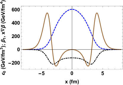
Figure 1: The initial energy density $\varepsilon_{0}$ (dashed), directed flow in $x$-direction $\beta^{1}$ (dash-dotted), and the divergence of directed flow $x\nabla^{i}\beta^{i}$ weighted by $x$ (solid line) as functions of coordinate $x$ at $y=0$ for Pb+Pb collisions at impact parameter $b=6$ fm.

Let us now explore these results numerically. We consider as an example Pb+Pb collisions. We model the shape of the charge fluctuation densities $\mu_{1,2}(x,y)$ by the nuclear thickness functions of the nuclei as given by Woods-Saxon distributions with appropriate radius $R_{A}$. We take nucleus $1$ to be traveling in the $+z$-direction with center at $x=b/2$ and nucleus $2$ to be traveling in the $-z$-direction with center at $x=-b/2$. Thus the primordial total angular momentum of the system at a finite total center of mass energy $\sqrt{s}$ is

$$L_{2}^{0}=-\frac{b}{2}\sqrt{s}\,,$$ (35)

and $L_{1}^{0}=0=L_{3}^{0}$. The primordial angular momentum is clockwise in the reaction plane, $L_{2}^{0}<0$.

The important quantities for the initial angular momentum after the collision are $\beta^{1}$ and $x\nabla^{i}\beta^{i}$. They are shown as functions of $x$ for collisions with impact parameter $b=6$ fm in Fig. 1. We note that $\beta^{1}$ is negative, i.e. for $\eta>0$ the directed flow is in the negative $x$-direction as expected for directed flow, and its contribution to the angular momentum $dL_{2}/d\eta$ is negative. We already know from Eq. (31) that the contribution from shear flow will have the opposite sign. That seems strange since that flow is opposing the motion of the initial nuclei. However, Fig. 1 makes it clear that $x\nabla^{i}\beta^{i}$ must have two nodes along the $x$-axis toward the outer regions of the fireball where its sign flips. In the inner regions the sign is indeed negative, leading to clockwise shear flow, while the outer regions exhibit a counter-clockwise shear flow. Upon integration over the transverse plane the counter-clockwise shear flow wins due to the weighting with the lever arm $x$.

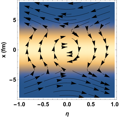
Figure 2: Energy flow components $(T^{01},T^{03})_{\mathrm{odd}}\sim(\tau\beta^{1},-\tau^{2}\nabla^{i}\beta^{i}/4)$ contributing to local angular momentum $dL_{2}/d\eta$, up to second order in time, plotted at $\tau=0.25$ fm/$c$ with the initial energy density $\varepsilon_{0}$ in the background, for Pb+Pb collisions at impact parameter $b=6$ fm.

Figure 3: The angular momentum per rapidity $dL_{2}/d\eta$ at $\eta=0$ at a time $\tau=0.25$ fm/$c$ as a function of impact parameter $b$ for Pb+Pb collisions as given by the leading terms in the power series in time.

An interesting picture emerges. Fig. 2 shows the part of the energy flow vector $(T^{01},T^{03})$ contributing to angular momentum in the reaction plane. To be precise, we plot the rapidity-even part of the 03-component and the rapidity-odd part of the 01-component, $(T^{01},T^{03})_{\text{odd}}=(T^{01}(\eta)-T^{01}(-\eta),T^{03}(\eta)+T^{03}(-\eta))/2$. This procedure drops terms proportional to $\alpha^{1}$ or $\nabla^{i}\alpha^{i}$ which act as a background here. We can clearly recognize the clockwise eddy current of energy flow at the center, and the counter-clockwise shear flow in the outer regions. Note that the nucleus in the top half ($x>0$) is moving to the right, the one at the bottom ($x<0$) is moving to the left.

In Fig. 3 we show the angular momentum $\mathrm{d}L_{2}/\mathrm{d}\eta$, at $\eta=0$, as a function of the impact parameter $b$ for Pb+Pb collisions. As expected the angular momentum of the gluon field goes to zero for $b=0$ and for $b\gg R_{A}$. Recall that this result holds for event averages with color fluctuation densities $\mu_{1,2}$, assumed to follow Woods-Saxon distributions. The shape of the curve is qualitatively consistent with the result from Becattini:2007sr in a setup inspired by the Glauber model. The numerical value of the angular momentum per rapidity is determined by the normalization of the initial energy density $\varepsilon_{0}$ and depends on time. For the former we have chosen $\varepsilon_{0}=605$ GeV/fm³ at a time $\tau=0.2$ fm/$c$ at the center for $b=6$ fm. This value has the correct order of magnitude for collisions at LHC energies but has not been tuned to data with any precision. One can estimate the relation between $\mathrm{d}L_{2}/\mathrm{d}\eta$ and the initial energy density $\varepsilon_{0}$ when one uses a simple approximation for the profile functions $\mu_{1,2}(x,y)$. Let us assume the profile functions represent simple slabs of radius $R_{A}$, with a fixed value $\bar{\mu}$ inside the slab. Then $\varepsilon_{0}$ is also a function describing a slab in the transverse plane with a value of $\bar{\varepsilon}_{0}\sim\bar{\mu}^{2}$ inside the overlap region of the nuclei. From Ref. Chen:2015wia we find

$$\beta^{1}=\varepsilon_{0}\frac{\mu_{1}\nabla^{1}\mu_{2}-\mu_{2}\nabla^{1}\mu_{1}}{\bar{\mu}^{2}}\\ =\varepsilon_{0}\left(-\delta(x-\partial_{2})-\delta(x-\partial_{1})\right)\;,$$ (36)

where $\partial_{i}$ here denotes the $x$-coordinate of the boundary of slab $i$ (at a fixed $y$) within the other slab. Note that the last expression means that we have approximated the realistic function $\beta^{1}(x)$ shown in Fig. 1 with two negative $\delta$-functions that replace the two negative peaks. We can easily integrate over $x$ and approximate the size of the fireball to be roughly $2R_{A}$ in $y$-direction. Thus we obtain approximately

$$\int\mathrm{d}^{2}r_{\perp}\beta^{1}\approx-4\bar{\varepsilon}_{0}R_{A}\;,$$ (37)

for $0<b<2R_{A}$, and we arrive at the final estimate

$$\frac{\mathrm{d}L_{2}}{\mathrm{d}\eta}\approx\frac{1}{2}\tau^{3}R_{A}\bar{\varepsilon}_{0}\left(1-\sinh^{2}\eta\right)\;.$$ (38)

This result should still hold approximately if we relax the assumption of slabs and treat $\bar{\varepsilon}_{0}$ as an average initial energy density of a system with more realistic transverse profiles. Let us emphasize once more, that despite the vortex aligned with the primordial total angular momentum, if integrated over the entire transverse plane $dL_{2}/d\eta>0$ is opposite to $L_{2}^{0}$. It is created by an ingoing longitudinal angular momentum flux, $dN_{2}/d\eta<0$ for $\eta>0$.

Lastly, let us note that in single events which deviate from the situation discussed here by fluctuations, could exhibit interesting additional local dynamics. Such calculations would have to be carried out numerically. However the global picture that we have presented here by integrating over the transverse plane should stay intact when transverse fluctuations are introduced.

III Matching to Fluid Dynamics

The energy momentum tensor of a system which is locally in full kinetic equilibrium can be written as

$$T_{\mathrm{id}}^{\mu\nu}=(e+p)u^{\mu}u^{\nu}-pg^{\mu\nu}\,,$$ (39)

where $e$ and $p$ are the local energy density and (equilibrium) pressure, related by the equation of state, and $u^{\mu}$ is the flow velocity of each local fluid cell as seen by the observer. Deviations from local kinetic equilibrium make it necessary to introduce dissipative corrections in the form of bulk stress $\Pi$ and shear stress tensor $\pi^{\mu\nu}$. The energy momentum tensor of viscous fluid dynamics can then be expressed as Muronga:2004sf

$$T_{\mathrm{vf}}^{\mu\nu}=(e+p+\Pi)u^{\mu}u^{\nu}-(p+\Pi)g^{\mu\nu}+\pi^{\mu\nu}\;,$$ (40)

where the tensor $\pi^{\mu\nu}$ is symmetric, traceless and orthogonal to the flow velocity, $u_{\mu}\pi^{\mu\nu}=0$. We have chosen to neglect additional conserved currents, such as baryon number, as we aim to match to a pure Yang-Mills system in this work. We have also lifted the ambiguity coming from the incomplete definition of a local rest frame by setting the heat flow $q^{\mu}=0$ to zero (Landau frame).

III.1 Matching to Ideal Fluid Dynamics

We will first discuss the case of a system undergoing rapid thermalization at a time $\tau_{\mathrm{th}}$, so that at the end of a rather short time period the energy momentum tensor can be written as in Eq. (39). It is assumed that during the short time interval in which local equilibrium is achieved, due to microscopic processes, the macroscopic evolution given by the flow of energy and momentum is negligible. In this instantaneous approximation we can hope to write the total energy momentum tensor as

$$T^{\mu\nu}_{\mathrm{tot}}=\Theta(\tau_{\mathrm{th}}-\tau)T^{\mu\nu}+\Theta(\tau-\tau_{\mathrm{th}})T_{\mathrm{id}}^{\mu\nu}\;,$$ (41)

where we have denoted the tensor before equilibration simply as $T^{\mu\nu}$, and $\Theta$ is the Heaviside step function.

Clearly not all energy momentum tensors can be written as an equilibrium tensor. Negative pressure, for example realized in Yang-Mills fields discussed here, see Eq. (19), cannot be accommodated in kinetic equilibrium. Thus the components of the energy momentum tensor must be permitted to change rapidly during the short equilibration phase. In order to constrain the local energy density $e$ and the 3-velocity $\mathbf{v}$, with $u^{\mu}=\gamma(1,\mathbf{v})$ at the end of this rapid equilibration process, we can use the fact that we have to satisfy energy and momentum conservation. Given the hierarchy of time scales in our assumptions we impose Fries:2005yc ; Fries:2007iy

$$\partial_{\mu}T^{\mu\nu}_{\mathrm{tot}}=0\,.$$ (42)

This condition provides four equations which equals the number of unknowns ($e,\mathbf{v})$. The pressure needs to be determined self-consistently in the equilibrated phase by the equation of state $p=p(e)$. Of course $\partial_{\mu}T^{\mu\nu}=0=\partial_{\mu}T^{\mu\nu}_{\mathrm{id}}$ and thus Eq. (42), works out to the simple condition

$$n_{\mu}T^{\mu\nu}=n_{\mu}T^{\mu\nu}_{\mathrm{id}}\,,$$ (43)

for $\nu=0,1,2,3$. Here $n_{\mu}=(\cosh\eta,0,0,-\sinh\eta)$ is the normal vector of the matching hypersurface $\tau=\tau_{\mathrm{th}}$. Hence, though energy and momentum are conserved at every point of the matching hypersurface, only the projection of $T^{\mu\nu}_{\mathrm{tot}}$ perpendicular to the matching surface is forced to be continuous at $\tau=\tau_{\mathrm{th}}$. Indeed, the longitudinal pressure in the case of the Yang-Mills energy momentum tensor from the last section matched to ideal fluid dynamics provides an example for non-continuous components.

In the case of a boost-invariant Yang-Mills energy momentum tensor as in the previous section, we can use the boost-symmetry and restrict ourselves to determining the fluid dynamic fields at the space-time rapidity slice $\eta=0$ only. Lorentz boosts then provide the result at any other $\eta$. We find a set of four equations

$$e= \,\varepsilon-\frac{S^{2}}{\varepsilon+p}\;,$$

$$\mathbf{v}= \,\frac{\mathbf{S}}{\varepsilon+p}\;,$$ (44)

where $\varepsilon=T^{00}$ and $S^{i}=T^{0i}$, for $i=1,2,3$, are the energy density and Poynting vector of the Yang-Mills system at midrapidity, respectively. Recall that the equation of state for the equilibrium pressure $p$ closes the system of equations.

Using the expressions up to second order in time from Eq. (19) the equations can be cast in the form Fries:2005yc ; Fries:2007iy

$$e= \,\varepsilon-\frac{\tau_{\mathrm{th}}^{2}}{4}\frac{\alpha^{2}+\frac{\tau_{\mathrm{th}}^{2}}{16}(\nabla^{k}\beta^{k})^{2}}{\varepsilon+p}\;,$$

$$v_{i}= \,\frac{\tau_{\mathrm{th}}}{2}\frac{\alpha^{i}}{\varepsilon+p}\,,\>i=1,2\,,$$ (45)

$$v_{3}= \,-\frac{\tau_{\mathrm{th}}^{2}}{8}\frac{\nabla^{k}\beta^{k}}{\varepsilon+p}\;,$$

$i=1,2$, with

$$\varepsilon=\varepsilon_{0}+\frac{\tau_{\mathrm{th}}^{2}}{8}\left(2\triangle\epsilon_{0}-\delta\right)\,.$$ (46)

First we notice that the rapidity-odd flow $\beta^{i}$ does not directly enter the expression for the transverse flow velocity $v_{i}$, for $i=1,2$. In fact the direction of the transverse fluid flow field $v_{i}$ is entirely determined by the direction of the Poynting vector at midrapidity, which is given by the rapidity-even flow $\alpha^{i}$. Information about directed flow is lost in the matching procedure, consistent with the possibility that individual components of the energy momentum tensor can be discontinuous on the matching hypersurface. On the other hand, the longitudinal velocity flow $v_{3}$ is directly proportional to the longitudinal gluon energy flow term $-\nabla^{i}\beta^{i}$. Therefore longitudinal shear flow is introduced into the fluid velocity field.

Turning to the angular momentum we note that $\partial_{\mu}T^{\mu\nu}=0$ for any symmetric energy momentum tensor automatically guarantees $\partial_{\lambda}M^{\mu\nu\lambda}=0$. So angular momentum is conserved at the matching surface. However, once more only the projection perpendicular to the matching hypersurface, $M^{\mu\nu\lambda}n_{\lambda}$, has to be continuous across $\tau=\tau_{\mathrm{th}}$. This ensures that the $\tau$-component of the $L_{2}$-flow in Milne coordinates,

$$\frac{\mathrm{d}H_{2}}{\mathrm{d}\eta}=\cos\eta\frac{\mathrm{d}L_{2}}{\mathrm{d}\eta}-\sinh\eta\frac{\mathrm{d}N_{2}}{\mathrm{d}\eta}\,$$ (47)

is smooth at matching. However, except at $\eta=0$, $\mathrm{d}L_{2}/\mathrm{d}\eta$ itself is not necessarily continuous across $\tau=\tau_{\mathrm{th}}$. It is straightforward to test the smoothness of $\mathrm{d}H_{2}/\mathrm{d}\eta$ at midrapidity explicitly using Eq. (45) in the calculation of $M^{\mu\nu\lambda}_{\mathrm{id}}$.

The matching to ideal fluid dynamics might seem academic, however it provides some features that generalize to viscous fluid dynamics. Moreover, an argument could be made that it is more physical than the popular procedure of matching to viscous fluid dynamics and then dropping dissipative stress terms. For the sake of studying the time evolution of angular momentum it will be preferable to match to viscous fluid dynamics while keeping dissipative stress, as discussed below.

III.2 Matching To Viscous Fluid Dynamics

The premise for matching to viscous fluid dynamics is different from the ideal case. The decomposition in Eq. (40) has in principle sufficient degrees of freedom and the Yang-Mills energy momentum tensor could be written directly as the energy momentum tensor of an off-equilibrium fluid. In other words one would directly seek a solution of the system of equations

$$T^{\mu\nu}_{\mathrm{YM}}=T^{\mu\nu}_{\mathrm{vf}}\;,$$ (48)

for the 10 independent unknown fields $e$, $p+\Pi$, $u^{\mu}$, $\pi^{\mu\nu}$. The separate determination of $p$ and $\Pi$ can be finalized after choosing an equation of state on the viscous fluid side. In this paradigm it is obvious that all components of the energy momentum tensor and the angular momentum tensor are continuous, and energy, momentum and angular momentum are trivially conserved at the matching time. However, to ensure these conservation laws the viscous fluid dynamics must be initialized with the dissipative stress obtained from the classical Yang-Mills phase.

The further approach of the system to equilibrium can then be calculated with suitable equations of motion for the viscous fluid. This could be standard Israel-Steward viscous fluid dynamics Israel:1979wp ; Heinz:2005bw or anisotropic fluid dynamics Martinez:2010sc ; Bazow:2013ifa . The latter might be more reliable with the large dissipative corrections we expect from a classical Yang-Mills system. In this work we focus on standard viscous fluid dynamics. We note that although the energy momentum tensor is continuous across the matching hypersurface, some of the equations of motion are not continuous.

In general, equation (48) might not allow a physically acceptable unique solution for the fluid fields. Acceptable here means that the physical conditions, $e>0$, $u^{2}=1$ with $u^{0}>0$, as well as $\pi^{\mu\nu}u_{\nu}=0$ are met. It is useful for practical purposes to use the eigenvalue property of the local rest frame

$$T^{\mu}_{\,\,\nu}u^{\nu}=eu^{\mu}\,,$$ (49)

and to state that Eq. (48) has a unique acceptable solution if Eq. (49) has a unique acceptable solution. We will solve Eq. (48) by first solving the eigenvalue problem Eq. (49). which has become standard practice for matching with fluid dynamics, even if the dissipative parts of the energy momentum tensor are later discarded.

We can proceed and determine the dissipative stress from

$$(p+\Pi)\left(u^{\mu}u^{\nu}-g^{\mu\nu}\right)+\pi^{\mu\nu}=T^{\mu\nu}_{\mathrm{YM}}-eu^{\mu}u^{\nu}\,,$$ (50)

and the equation of state $p=p(e)$. We can further decompose the contributions to the left hand side by taking the trace,

$$p+\Pi=\frac{1}{3}\left(e-T^{\mu}_{\mathrm{YM},\mu}\right)\,.$$ (51)

In the classical Yang-Mills case the initial energy momentum tensor is conformal and thus the bulk stress is fixed to one third of the interaction measure $e-3p$ of the fluid after matching.

We now proceed with a decomposition of the classical Yang-Mills energy momentum tensor obtained from the McLerran-Venugopalan model. We keep the matching time $\tau_{0}$ as a parameter, but it is clear that for any practical applications $\tau_{0}$ needs to be chosen before the growth of fluctuations could significantly alter the classical solutions. In addition, for the analytic solutions discussed here, $\tau_{0}$ should be within the convergence radius of the power series in time.

The determination of the viscous fluid fields from Eq. (19) is preferably done numerically on the fluid dynamics grid. However it might be instructive to briefly study one particular case analytically, namely the center of a smooth, event-averaged collision at midrapidity. In that case the symmetry arguments collected in Tab. 1 apply and the energy momentum tensor in its Cartesian components reads

$$T^{\mu\nu}_{\mathrm{YM},0}=\begin{pmatrix}\varepsilon_{0}-\frac{\tau_{0}^{2}}{8}(-2\triangle\epsilon_{0}+\delta)&0&0&0\\ 0&\varepsilon_{0}-\frac{\tau_{0}^{2}}{4}(-\triangle\varepsilon_{0}+\delta-\omega)&0&\frac{1}{2}\tau\beta^{1}\\ 0&0&\varepsilon_{0}-\frac{\tau_{0}^{2}}{4}(-\triangle\varepsilon_{0}+\delta+\omega)&0\\ 0&\frac{1}{2}\tau\beta^{1}&0&-\varepsilon_{0}+\frac{\tau_{0}^{2}}{8}(-2\triangle\varepsilon_{0}+3\delta)\end{pmatrix}+\mathcal{O}(\tau^{4})\,.$$ (52)

As expected from symmetry arguments the velocity $u^{\mu}=(1,0,0,0)$ corresponds to an eigenvector with rest frame energy $e$ which precisely resembles the lab frame energy $T^{00}_{\mathrm{YM}}$:

$$e=\varepsilon_{0}-\frac{\tau_{0}^{2}}{8}\left(-2\triangle\varepsilon_{0}+\delta\right)\,.$$ (53)

One can check that this is the only physically acceptable solution to the pertinent eigenvalue problem. From Eq. (51) we know $p+\Pi=e/3$ and the traceless part of Eq. (50) yields the shear stress tensor,

$$\small{\pi^{\mu\nu}=\begin{pmatrix}0&0&0&0\\ 0&\frac{2}{3}e-\frac{\tau_{0}^{2}}{8}\delta+\frac{\tau_{0}^{2}}{4}\omega&0&\frac{1}{2}\tau_{0}\beta^{1}\\ 0&0&\frac{2}{3}e-\frac{\tau_{0}^{2}}{8}\delta-\frac{\tau_{0}^{2}}{4}\omega&0\\ 0&\frac{1}{2}\tau_{0}\beta^{1}&0&-\frac{4}{3}e+\frac{\tau_{0}^{2}}{4}\delta\end{pmatrix}}\,.$$ (54)

We can make a few basic observations that turn out to hold numerically for other points besides the center. We observe that the rapidity-odd flow $\beta^{i}$ translates directly into transverse flow of viscous stress $\pi^{0i}$, for $i=1,2$. It does not appear in the transverse flow velocity $u^{i}$. This is an immediate consequence of boost-invariance. Boost-symmetry does not permit rapidity-odd transverse 4-vectors, but rapidity-odd transverse flow components are allowed in rank-2 tensors. However, the longitudinal gluon energy flow term $\nabla^{i}\beta^{i}$ directly translates into longitudinal fluid flow $v_{3}$, although it just happens to vanish at the center point. A system without boost-invariance would not have the restriction on the transverse flow field. However, for very large collision energies we would expect our observations in the boost-invariant case to be a valid approximation around midrapidity.

IV Evolution of Initial Angular Momentum in Viscous Fluid Dynamics

IV.1 Initial Conditions

Now let us discuss some numerical results for the matching of the classical Yang-Mills energy tensor to viscous fluid dynamics. As a representative example we continue to study Pb+Pb collisions with an impact parameter of $b=6$ fm as before. We set the matching time to $\tau_{0}=0.1$ fm/$c$ and choose $Q=1$ GeV in the analytic expressions up to second order in $\tau$. We set the second order terms $\omega=0=\gamma$ here for simplicity. These terms would lead to a pressure asymmetry in the transverse plane which shall be studied elsewhere. They do not contribute to $dL_{2}/d\eta$.

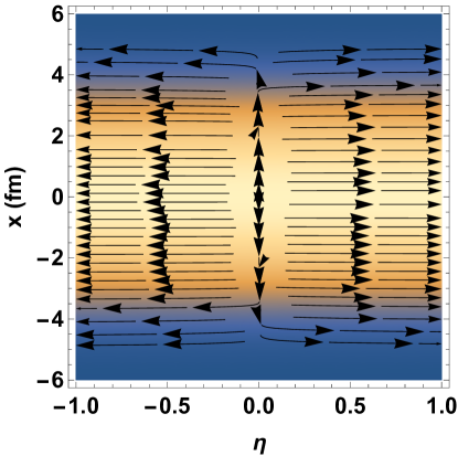
Figure 4: Fluid flow vector field in the reaction plane, $(v_{1},v_{3})$, together with the local fluid energy density $e$ obtained from the matching at $\tau=0.1$ fm/$c$ as described in the text for Pb+Pb collisions at impact parameter $b=6$ fm. The flow is dominated by the Bjorken expansion.

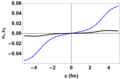
Figure 5: Fluid flow vector components $v_{1}$ (dashed blue line) and $v_{3}$ (solid black line) as functions of $x$ at $\eta=0$, $y=0$ obtained from the matching at $\tau=0.1$ fm/$c$ as described in the text for Pb+Pb collisions at impact parameter $b=6$ fm. Because of the quadratic time-dependence of the longitudinal shear flow the build-up of $v_{3}$ is lagging behind $v_{1}$.

Fig. 4 shows the local energy density $e(\eta,x)$ together with the flow velocity vector $\mathbf{v}(\eta,x)$ in the reaction plane. Predictably the flow is dominated by the longitudinal Bjorken expansion $v_{3}\approx\tanh\eta$. Only around midrapidity can the effect of transverse flow be competitive. Note that “naive” boost-invariant fluid dynamics, as it has been practiced in 2+1D fluid dynamics codes for many years, restricts itself to precisely $v_{3}=\tanh\eta$, which does not cover all allowed boost-invariant solutions. The longitudinal shear flow is an example for a deviation from this naive scenario. It can be visualized by the behavior of the $z$-component of the fluid velocity, $v_{3}$, in the plane $\eta=0$. Fig. 5 shows $v_{1}$ and $v_{3}$ plotted along the $x$-axis at $\eta=0$. The radial flow at this early time takes maximum values around $\sim 0.05\,c$ on the surface of the system. The size of $v_{3}$ at this early time is about an order of magnitude suppressed, but it grows quadratically with time while the transverse flow velocity $v_{1}$ grows linearly. Interestingly, unlike the energy flow $T^{03}$ there are no nodes in $v_{3}$ away from the center. Moreover, the direction of $v_{3}$ goes in the “right” direction, i.e. along the direction of motion of the nuclei. That means that the shear flow opposite to the nuclear motion, observed in the previous section, must be carried by the dissipative stress tensor.

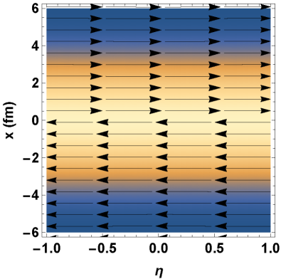
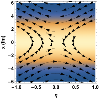
Figure 6: The flow of energy in the reaction plane for Pb+Pb collisions at impact parameter $b=6$ fm, at time $\tau=0.1$ fm/$c$. Left panel: the part of the ideal energy momentum tensor contributing to angular momentum, $(T_{\text{id}}^{01},T_{\text{id}}^{03})_{\text{odd}}$. Right panel: the same for the shear stress tensor, $(\pi^{01},\pi^{03})_{\text{odd}}$. Only the rapidity-even part of longitudinal flow and the rapidity-odd part of transverse flow contribute to angular momentum. The ideal part exhibits longitudinal shear flow aligned with the motion of the nuclei. The dissipative part carries directed flow aligned with, and longitudinal shear flow opposite to, the motion of the nuclei.

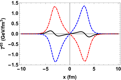
Figure 7: The longitudinal energy flow $T^{03}$ as a function of $x$ at $\eta=0$ and $y=0$. As in Fig. 6 the ideal contribution (dashed blue line) and the dissipative contribution (dot-dashed red line) are shown separately. The total energy flow (solid black line), with the two additional nodes as discussed in the text, emerges from a non-trivial cancellation of the ideal and dissipative contributions.

To separate the two contributions clearly we show in Fig. 6 separately the ideal part and the dissipative part of the energy flow in the reaction plane,

$$\left(T_{\mathrm{id}}^{01},T_{\mathrm{id}}^{03}\right)=\left(e+p\right)\gamma^{2}(v_{1},v_{3})\, \text{(left panel)}\,,$$ (55)

$$\left(\pi^{01},\pi^{03}\right)\, \text{(right panel)}\,,$$ (56)

respectively. In both cases, for clarity, we again only plot the part of the flow field that carries angular momentum, i.e. the rapidity-even part of the 03-component and the rapidity-odd part of the 01-component, formally defined in the previous section. As we expected from Fig. 5 the ideal part of the fluid only exhibits shear flow, whose direction is consistent with the total system angular momentum. The dissipative stress tensor carries the directed flow in transverse direction, and a longitudinal shear flow opposing the velocity field. Note that both contributions have to add up to the total energy flow field and angular momentum discussed in Sec. II.2. We thus expect the dissipative longitudinal shear flow to be dominant. Indeed, in Fig. 7, $T^{03}=T^{03}_{\mathrm{id}}+\pi^{03}$ is plotted along the $x$-axis in the $\eta=0$ plane. We show the ideal part, which basically traces the line of $v_{3}$ in Fig. 5, and the dissipative part separately, together with the total. The ideal and dissipative part have opposite sign and partly cancel each other to give the total energy flow with the two additional nodes as discussed before.

We conclude that the decomposition of the angular momentum in terms of fluid fields yields a non-trivial separation of flow and angular momentum between the ideal and the dissipative part of the energy momentum tensor. Neglecting the shear stress tensor at the point of matching could alter the angular momentum and other macroscopic quantities significantly. This is plainly visible in Figs. 8 and 9 which are discussed in detail in the next subsection.

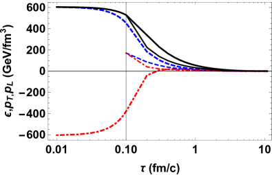
Figure 8: The time evolution of energy density (solid), transverse pressure (dashed) and longitudinal pressure (dash-dotted line) as a function of time $\tau$ at the center $(x,y,\eta)=(0,0,0)$ of a Pb+Pb collision with $b=6$ fm. For the evolution before $\tau_{0}=0.1$ fm/$c$ we use our classical Yang-Mills formalism. After that time the system is evolved with the relativistic viscous hydro code VIRAL in two configurations: (a) dissipative stress is carried over from the classical Yang-Mills simulation to viscous fluid dynamics (thick lines), (b) dissipative stress is discarded at the beginning of the fluid dynamic simulation. In the latter case longitudinal and transverse pressure are discontinuous at the matching time and the system cools much faster at the center of the collision.

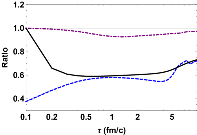
Figure 9: For the same system as shown in Fig. 8 we show the ratio of energy densities in cases (b) and (a) discussed in the text (without and with initial dissipative stress; black solid line) and the ratio of transverse pressures in case (b) and (a) (blue dash-dotted line) as a function of time $\tau$. The energy density and pressure are calculated in VIRAL fluid dynamics and taken at the center of the collision $(x,y,\eta)=(0,0,0)$. Recall that the absence of dissipative stress here refers to the procedure of discarding the shear and bulk stress found from classical Yang-Mills fields at $\tau=0.1$ fm/$c$. We also show the same ratio for the transverse velocity component $v_{1}$ measured at a point $(x,y,\eta)=(4\,\text{fm},0,0)$ away from the center. Discarding the initial dissipative stress leads to a 30-40% decrease in energy density and transverse pressure at a given time over the entire time evolution. At the same time the transverse velocity is reduced by 5-10%.

Figure 10: The time evolution of the ratio $T^{03}/T^{00}$ as a function of time $\tau$ at the center point $(x,y,\eta)=(-4\,\text{fm},0,0)$ in a Pb+Pb collision with $b=6$ fm. Again we have used our classical Yang-Mills formalism before time $\tau_{0}=0.1$ fm/$c$ and after that time we use the relativistic viscous hydro code VIRAL with initial dissipative stress.

IV.2 Evolution In The Fluid Phase

One can give simple qualitative arguments about the subsequent evolution of angular momentum in viscous fluid dynamic given initial conditions as discussed in the previous subsection. Here we briefly discuss those arguments and follow up with a numerical simulation using the Texas VIscous RelAtivistic fLuid (VIRAL) code, see Appendix A. We evolve the system in fluid dynamics with two different initializations: (a) with shear and bulk stress at the matching time carried over from the classical Yang-Mills phase, and (b) with shear and bulk stress discarded at the matching time. While case (a) seems to be the more physical one, an argument could be made that case (b) is an acceptable approximation. Even in case (b) bulk and shear stress build up with time, driven by the gradients in the system, as long as bulk and shear viscosities are finite. In fact, interestingly we find that the Navier-Stokes values $\pi^{\mu\nu}_{\mathrm{NS}}=2\eta d^{\langle\mu}u^{\nu\rangle}$ for the shear stress, calculated from the initial flow field at the matching time, are remarkably similar to the true values $\pi^{\mu\nu}$ extracted from the classical Yang-Mills system. To be more precise, components of the two tensors qualitatively have the same functional dependence on position, and the same sign. One could roughly write $\pi^{\mu\nu}\approx C\pi^{\mu\nu}_{\mathrm{NS}}$ with $C>0$. $C$ varies from component to component but is generally of order one if minimal viscosities are used in the Navier-Stokes approximation. Here we need to define

$$d^{\langle\mu}u^{\nu\rangle}=\frac{1}{2}\left(d^{\mu}u^{\nu}+d^{\nu}u^{\mu}\right)-\frac{1}{3}\Delta^{\mu\nu}d_{\mu}u^{\mu}\,,$$ (57)

where $\Delta^{\mu\nu}=g^{\mu\nu}-u^{\mu}u^{\nu}$ is the usual projection operator orthogonal to the flow velocity, and $d^{\mu}=\Delta^{\mu}_{\nu}\partial^{\nu}$ Muronga:2004sf . The argument in favor of (b) would be that the second order corrections in viscous fluid dynamics, $\pi^{\mu\nu}-\pi^{\mu\nu}_{\mathrm{NS}}$, should be small. In practice, this difference matters greatly at early matching times.

Quantitatively there are sizable differences between running VIRAL for scenarios (a) and (b). Fig. 8 shows the evolution of energy density, transverse pressure and longitudinal pressure at the center of the collision $(x,y,\eta)=(0,0,0)$ as a function of time. Note that the lab frame and local fluid rest frame coincide at the point shown and we plot both the evolution in the classical Yang-Mills phase ($\tau<0.1$ fm) and the viscous fluid phase ($\tau>0.1$ fm) in case (a). Per our matching procedure energy densities and pressures evolve smoothly across the matching time $\tau_{0}$. The VIRAL code is stable although the longitudinal pressure is still negative at initialization. Of course, higher order gradient corrections to second order viscous fluid dynamics, not included here, could potentially be large. For $\tau>\tau_{0}$ we also show the results of initializing VIRAL in case (b), when the initial dissipative stress is discarded. The energy density and pressure are now permitted to be discontinuous and indeed exhibit large jumps at $\tau_{0}$. The energy density is continuous here only due to the fact that at the chosen point at the center the local rest frame is also the lab frame which enforces $\pi^{00}=0$ by construction. We notice that the system cools much faster and at the same time has a lower transverse pressure and larger longitudinal pressure compared to case (a).

The comparison is continued in Fig. 9 where the ratio of cases (b) and (a) is plotted for the energy density and transverse pressure at the center, and for the transverse velocity at a point 5 fm away from the center. The faster cooling and reduced transverse pressure in case (b) are clearly visible and persist to very late times. The effect on the transverse velocity is not as pronounced, case (b) lags behind case (a) by about 5-10%. The discrepancy might decrease if later matching times are chosen, although the validity of the classical Yang-Mills approach becomes doubtful. In any case, keeping the dissipative stress when initializing the fluid dynamics is the preferred method, despite uncertainties coming from large gradients.

Let us discuss the fate of angular momentum. The first observation is that shear viscosity will dampen the longitudinal shear flow shown in the left panel of Fig. 6. At the same time the shear stress tensor will relax to its Navier-Stokes value $\pi_{\mathrm{NS}}^{\mu\nu}$. At the beginning of the fluid dynamic evolution the angular momentum in the shear stress tensor is carried by the rapidity-odd part of $\pi^{01}$ and the rapidity-even part of $\pi^{03}$. It is easy to check that boost-symmetry ensures that the corresponding Navier-Stokes quantities, the rapidity-odd part of $\pi^{01}_{\mathrm{NS}}$ and the rapidity-even part of $\pi^{03}_{\mathrm{NS}}$ vanish. Thus the flow carrying angular momentum on the right hand side of Fig. 6 will be damped.

In summary, from simple arguments we expect that longitudinal shear flow and the angular momentum density at midrapidity tend to die out in the viscous fluid phase of a system with exact boost-invariance. The longitudinal flow of angular momentum, $dN_{2}/d\eta$ in early fluid dynamics is thus reversed compared to the Yang-Mills phase. Our expectations are confirmed by running the VIRAL fluid code. Fig. 10 presents a typical example for the time evolution of the longitudinal shear flow. The ratio $T^{03}/T^{00}$ at a point at midrapidity but away from the center of the transverse plane is depicted as a function of time in case (a). The matching from classical Yang-Mills evolution to fluid dynamics is smooth but leads to a rapid change of the time derivative which dissipates the shear flow. Thus, even though matching procedure (a) ensures continuity and macroscopic conservation laws, we have an explicit example of a non-smooth time evolution. This is not unexpected as important microscopic physics is missing when Gauss’ Law is instantaneously replaced by a dissipative law at time $\tau_{0}$.

Let us for a moment look at the larger picture. Realistic systems obey boost-invariance only around mid-rapidity and the total angular momentum of the system is finite and constant. The arguments given above will still hold approximately around midrapidity, but will fail away from midrapidity. Under realistic conditions the flow field can support directed flow which corresponds to a rotational motion of the system. Indeed, experimental measurements see that quantities directly sensitive to angular momentum, e.g. the directed flow of particles Adamczyk:2014ipa , and the polarization of $\Lambda$ hyperons STARLambda notably decrease at midrapidity with increasing collision energy. They are suppressed by the increasingly well realized boost-invariance. A quantitative study of these effects will require a description of the initial state with a realistic rapidity profile, and its dependence on the collision energy. Lastly, we mention that boost-invariance prevents fluctuations of the fluid dynamic system in longitudinal direction. Such fluctuations can lead to Kelvin-Helmholtz instabilities and the formation of smaller vortices in the fluid phase Csernai:2011qq ; Okamoto:2017ukz .

V Conclusions

In summary, we have estimated the event-averaged angular momentum in nuclear collisions as a function of space-time rapidity, within in the McLerran-Venugopalan model of classical gluon fields, at very early times $\lesssim 1/Q_{s}$. The results can serve as estimates around midrapidity for realistic collisions at top RHIC energies and higher, where boost-invariance holds approximately. We find that $dL_{2}/d\eta$ peaks in mid-central collisions for $b\approx 5$ fm for collisions of Pb nuclei. From Eq. (38) we read off that $dL_{2}/d\eta\approx\frac{1}{2}R_{A}Q_{s}^{-3}\bar{\varepsilon}_{0}$ at time $\tau\approx 1/Q_{s}$ at midrapidity. The build-up of angular momentum at midrapidity is driven by the QCD version of Gauss’ Law. The angular momentum can be visualized as a vortex in the gluon energy flow in the reaction plane, with an opposing longitudinal shear flow of energy. The net effect is angular momentum $dL_{2}/d\eta$ opposite to the total primordial angular momentum.

We have discussed the direct matching of classical gluon fields at early time to relativistic fluid dynamics, following established precedence. We have derived some fundamental statements both regarding matching to ideal and second order viscous fluid dynamics. If conservation laws for energy, momentum and angular momentum are used as the guiding principle the projection of the energy momentum tensor perpendicular to the matching hypersurface is always continuous. In ideal fluid dynamics other components might be discontinuous while viscous fluid dynamics allows for a smooth energy momentum tensor across the matching. However, dissipative stress needs to be kept in the fluid initial conditions to ensure macroscopic conservation laws and continuous energy momentum and angular momentum tensors. As a caveat we have pointed out that even if dissipative stress is kept some equations of motion are discontinuous across the matching surface. Shear in the longitudinal energy flow is a relevant example, with the time derivative changing sign abruptly around the matching time. Thus the total amount of angular momentum built up at midrapidity depends critically on the matching time chosen. A more reliable estimate would have to take into account how the macroscopic mechanism of Gauss’ Law is broken by the onset of decoherence of the classical fields. We will also mention once more that second order viscous fluid dynamics will evolve systems with large initial shear stress with significant uncertainties which can be checked by comparing to anisotropic fluid codes.

In the subsequent fluid dynamic evolution angular momentum is initially carried by the longitudinal shear flow and by directed flow in the shear stress tensor. This is dictated by boost-invariance. Both modes are damped in viscous fluid dynamics. As a result the angular momentum around midrapidity decays quickly with time. This result is consistent with small or vanishing directed flow and particle polarization seen at top RHIC energies.

Although the final angular momentum is small, there are several conclusions we can draw. First, we have clarified the mechanism through which angular momentum can be transported to midrapitity in the initial CGC phase. Secondly, we have described the very simple mechanisms through which the angular momentum dissipates in a boost-invariant fluid system. We emphasize once more that angular momentum is conserved throughout the entire calculation, however the total amount of angular momentum in the boost-invariant system is not well defined. Our study can serve as a starting point for calculations at lower collision energies or at larger rapidities, e.g. if boost-invariance is explicitly broken with additional assumptions in the fluid dynamic phase. This would allow for directed flow at larger rapidities. In the future, event-by-event calculations should also study the effect of fluctuations.

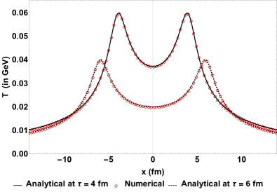
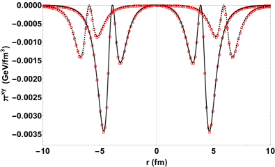
Figure 11: Analytic results (black solid lines) and results obtained with the VIRAL code (red circles) for the cold plasma limit problem described in Marrochio:2013wla . We show the temperature profile along the $x$-axis (upper panel) and the shear stress component $\pi^{xy}$ along a line $x=y$ (lower panel) at midrapidity for times 4 fm/$c$ and 6 fm/$c$. The system is initialized at time 1 fm/$c$.

*

Appendix A The VIRAL Fluid Code

For this work we have utilized the VIscous RelAtivistic fLuid (VIRAL) code developed locally. We will introduce details of this code in more detail elsewhere, but we want to briefly summarize its technical specifications and abilities. VIRAL solves the equations of motion of second order viscous relativistic fluid dynamics in 3+1 dimensions Israel:1979wp ; Muronga:2004sf ; Schenke:2010nt ; Karpenko:2013wva , written as conservation laws with source terms. Only five independent components of the shear stress tensor are treated as dynamical quantities, the remaining components are reconstructed from constraints. The conservation laws are solved through the improved fluxes suggested by Kurganov and Tadmor KurTad:2000 , using 5th order WENO (weighted essentially non-oscillatory) spatial derivatives weno . The time integration is carried out with a 3rd order TVD (total variation diminishing) Runge-Kutta scheme tvdrk . The code is written in C++ with built in MPI capabilities. For the calculations in Sec. IV we have used the equation of state s95p-PCE165-v0 Huovinen:2009yb ; eos:huovinen , and constant specific shear viscosity $\eta/s=1/4\pi$ and specific bulk viscosity $\zeta/s=0.01/4\pi$.

In order to offer a quick but non-trivial check of the code we present results of a test desribed in Marrochio:2013wla based on the work by Gubser et al. Gubser:2010ze ; Gubser:2010ui . In Fig. 11 we show analytic results for the temperature and one component of the shear stress tensor in the cold plasma limit discussed in Marrochio:2013wla , together with results obtained with VIRAL for the same setup. The VIRAL results are virtually indistinguishable from the analytic results despite the steep gradients. For this test the code was run with a conformal equation of state $e=3p$ and $\eta/s=0.2$. For details of the problem solved here we refer the reader to Marrochio:2013wla .

- (1) L. Adamczyk et al. (STAR Collaboration), preprint arXiv:1701.06657.
- (2) Z. T. Liang and X. N. Wang, Phys. Rev. Lett. 94, 102301 (2005), erratum Phys. Rev. Lett. 96, 039901 (2006).
- (3) L. P. Csernai, V. K. Magas and D. J. Wang, Phys. Rev. C 87, 034906 (2013).
- (4) F. Becattini, L. Csernai and D. J. Wang, Phys. Rev. C 88, 034905 (2013), erratum Phys. Rev. C 93, 069901 (2016).
- (5) Y. Jiang, Z. W. Lin and J. Liao, Phys. Rev. C 94, 044910 (2016), erratum Phys. Rev. C 95, 049904 (2017).
- (6) L. G. Pang, H. Petersen, Q. Wang and X. N. Wang, Phys. Rev. Lett. 117, 192301 (2016).
- (7) W. T. Deng and X. G. Huang, Phys. Rev. C 93, 064907 (2016).
- (8) Y. Xie, D. Wang and L. P. Csernai, Phys. Rev. C 95, 031901 (2017).
- (9) L. D. McLerran and R. Venugopalan, Phys. Rev. D 49, 3352 (1994).
- (10) L. D. McLerran and R. Venugopalan, Phys. Rev. D 49, 2233 (1994).
- (11) J. Jalilian-Marian, A. Kovner, L. D. McLerran and H. Weigert, Phys. Rev. D 55, 5414 (1997).
- (12) A. Kovner, L. D. McLerran and H. Weigert, Phys. Rev. D 52, 3809 (1995).
- (13) A. Kovner, L. D. McLerran and H. Weigert, Phys. Rev. D 52, 6231 (1995).
- (14) Y. V. Kovchegov, Phys. Rev. D 54, 5463 (1996).
- (15) Y. V. Kovchegov and A. H. Mueller, Nucl. Phys. B 529, 451 (1998).
- (16) E. Iancu and R. Venugopalan, in Quark Gluon Plasma 3, ed. R. C. Hwa and X.-N. Wang, World Scientific (2003).
- (17) F. Gelis, E. Iancu, J. Jalilian-Marian and R. Venugopalan, Ann. Rev. Nucl. Part. Sci. 60, 463 (2010).
- (18) F. Becattini, F. Piccinini and J. Rizzo, Phys. Rev. C 77, 024906 (2008).
- (19) F. Becattini, I. Karpenko, M. Lisa, I. Upsal and S. Voloshin, Phys. Rev. C 95, 054902 (2017).
- (20) I. Karpenko and F. Becattini, Eur. Phys. J. C 77, 213 (2017).
- (21) H. Li, H. Petersen, L. G. Pang, Q. Wang, X. L. Xia and X. N. Wang, preprint arXiv:1704.03569 [nucl-th].
- (22) R. J. Fries, J. I. Kapusta and Y. Li, preprint nucl-th/0604054.
- (23) G. Chen and R. J. Fries, Phys. Lett. B 723, 417 (2013).
- (24) G. Chen, R. J. Fries, J. I. Kapusta and Y. Li, Phys. Rev. C 92, 064912 (2015).
- (25) M. Li and J. I. Kapusta, Phys. Rev. C 94, 024908 (2016).
- (26) K. Dusling, F. Gelis and R. Venugopalan, Nucl. Phys. A 872, 161 (2011).
- (27) J. Berges, K. Boguslavski, S. Schlichting and R. Venugopalan, Phys. Rev. D 89, 074011 (2014).
- (28) J. Berges, K. Boguslavski, S. Schlichting and R. Venugopalan, Phys. Rev. D 89, 114007 (2014).
- (29) W. Israel and J. M. Stewart, Annals Phys. 118, 341 (1979).
- (30) A. Muronga and D. H. Rischke, preprint nucl-th/0407114.
- (31) U. W. Heinz, H. Song and A. K. Chaudhuri, Phys. Rev. C 73, 034904 (2006).
- (32) P. Romatschke and U. Romatschke, Phys. Rev. Lett. 99, 172301 (2007).
- (33) K. Dusling and D. Teaney, Phys. Rev. C 77, 034905 (2008).
- (34) B. Schenke, S. Jeon and C. Gale, Phys. Rev. C 82, 014903 (2010).
- (35) I. Karpenko, P. Huovinen and M. Bleicher, Comput. Phys. Commun. 185, 3016 (2014).
- (36) B. Schenke, P. Tribedy and R. Venugopalan, Phys. Rev. Lett. 108, 252301 (2012).
- (37) B. Schenke, P. Tribedy and R. Venugopalan, Phys. Rev. C 86, 034908 (2012).
- (38) C. Gale, S. Jeon, B. Schenke, P. Tribedy and R. Venugopalan, Phys. Rev. Lett. 110, 012302 (2013).
- (39) W. van der Schee, P. Romatschke and S. Pratt, Phys. Rev. Lett. 111, 222302 (2013).
- (40) M. Martinez and M. Strickland, Nucl. Phys. A 848, 183 (2010).
- (41) D. Bazow, U. W. Heinz and M. Strickland, Phys. Rev. C 90, 054910 (2014).
- (42) F. Gelis, T. Lappi and R. Venugopalan, Phys. Rev. D 78, 054019 (2008).
- (43) L. P. Csernai and J. H. Inderhaug, Int. J. Mod. Phys. E 24, 1550013 (2015).
- (44) A. Krasnitz and R. Venugopalan, Phys. Rev. Lett. 86, 1717 (2001).
- (45) T. Lappi, Phys. Rev. C 67, 054903 (2003).
- (46) A. Krasnitz, Y. Nara, and R. Venugopalan, Nucl. Phys. A 727, 427 (2003).
- (47) R. J. Fries, J. I. Kapusta, and Y. Li, Nucl. Phys. A 774, 861 (2006).
- (48) T. Lappi, Phys. Lett. B 643, 11 (2006).
- (49) P. Romatschke and J. D. Hogg, JHEP 1304, 048 (2013).
- (50) R. J. Fries, J. Phys. G 34, S851 (2007).
- (51) L. Adamczyk et al. [STAR Collaboration], Phys. Rev. Lett. 112, 162301 (2014).
- (52) L. P. Csernai, D. D. Strottman and C. Anderlik, Phys. Rev. C 85, 054901 (2012).
- (53) K. Okamoto and C. Nonaka, preprint arXiv:1703.01473 [nucl-th].
- (54) A. Kurganov, E. Tadmor, J. Comp. Phys. 160, 241 (2000).
- (55) C. W. Shu, in Advanced Numerical Approximation of Nonlinear Hyperbolic Equations, Springer (1998).
- (56) S. Gottlieb and C. W. Shu, Math. Comp. 67, 73 (1998).
- (57) P. Huovinen and P. Petreczky, Nucl. Phys. A 837, 26 (2010).
- (58) P. Huovinen, https://wiki.bnl.gov/TECHQM/index.php/ QCD_Equation_of_State, accessed May 15,2017.
- (59) H. Marrochio, J. Noronha, G. S. Denicol, M. Luzum, S. Jeon and C. Gale, Phys. Rev. C 91, 014903 (2015).
- (60) S. S. Gubser, Phys. Rev. D 82, 085027 (2010).
- (61) S. S. Gubser and A. Yarom, Nucl. Phys. B 846, 469 (2011).