Constraining sleptons at the LHC in a supersymmetric low-scale seesaw scenario

Abstract

We consider a scenario inspired by natural supersymmetry, where neutrino data is explained within a low-scale seesaw scenario. We extend the Minimal Supersymmetric Standard Model by adding light right-handed neutrinos and their superpartners, the R-sneutrinos, and consider the lightest neutralinos to be higgsino-like.
We consider the possibilities of having either an R-sneutrino or a higgsino as lightest supersymmetric particle. Assuming that squarks and gauginos are heavy, we systematically evaluate the bounds on slepton masses due to existing LHC data.

1 Introduction

The discovery of the Higgs boson in the 8 TeV run of the LHC Aad:2012tfa ; Chatrchyan:2012xdj marks one of the most important milestones in particle physics. Its mass is already known rather precisely: $m_{h}=125.09\pm 0.21$ (stat.) $\pm 0.11$ (syst.) GeV Aad:2015zhl , and the signal strength of various LHC searches has been found consistent with the SM predictions. While this completes the Standard Model (SM) particle-wise, several questions still remain open, for example: (i) Is it possible to include the SM in a grand unified theory where all gauge forces unify? (ii) Is there a particle physics explanation of the observed dark matter relic density? (iii) What causes the hierarchy in the fermion mass spectrum and why are neutrinos so much lighter than the other fermions? What causes the observed mixing patterns in the fermion sector? (iv) What stabilizes the Higgs mass at the electroweak scale?

Supersymmetric models address several of these questions and thus the search for supersymmetry (SUSY) is among the main priorities of the LHC collaborations. Up to now no significant sign for physics beyond SM has been found. The combination of the Higgs discovery with the (yet) unsuccessful searches has led to the introduction of a model class called ‘natural SUSY’ Brust:2011tb ; Papucci:2011wy ; Hall:2011aa ; Blum:2012ii ; Espinosa:2012in ; D'Agnolo:2012mj ; Baer:2012uy ; Younkin:2012ui ; Kribs:2013lua ; Hardy:2013ywa ; Kowalska:2013ica ; Han:2013kga . Here, the basic idea is to give electroweak-scale masses only to those SUSY particles giving a sizeable contribution to the mass of the Higgs boson, such that a too large tuning of parameters is avoided. All other particle masses are taken at the multi-TeV scale. In particular, masses of the order of a few hundred GeV up to about one TeV are assigned to the higgsinos (the partners of the Higgs bosons), the lightest stop (the partner of the top-quark) and, if the latter is mainly a left-stop, also to the light sbottom. In addition the gluino and the heavier stop masses should also be close to at most a few TeV.

Neutrino oscillation experiments confirm that at least two neutrinos have a non-zero mass. The exact mass generation mechanism for these particles is unknown, and both the SM and the MSSM remain agnostic on this topic. Although many ways to generate neutrino mass exist, perhaps the most popular one is the seesaw mechanism Minkowski:1977sc ; Yanagida:1979as ; Mohapatra:1979ia ; GellMann:1980vs ; Schechter:1980gr ; Foot:1988aq . The main problem with the usual seesaw mechanisms lies on the difficulty in testing its validity. In general, if Yukawa couplings are sizeable, the seesaw relations require Majorana neutrino masses to be very large, such that the new heavy states cannot be produced at colliders. In contrast, if one requires the masses to be light, then the Yukawas need to be small, making production cross-sections and decay rates to vanish. A possible way out of this dilemma lies on what is called the inverse seesaw Mohapatra:1986bd , which is based on having specific structures on the mass matrix (generally motivated by symmetry arguments) to generate small neutrino masses. This, at the same time, allows Yukawa couplings to be large, and sterile masses to be light.

We consider here a supersymmetric model where neutrino data are explained via a minimal inverse seesaw scenario where the gauge-singlet neutrinos have masses in the range $\mathcal{O}\left({{\rm keV}}\right)$ to $\mathcal{O}\left({100~{}{\rm GeV}}\right)$. We explore this with a parametrization built for the standard seesaw, and go to the limit where the inverse seesaw emerges, such that Yukawas and mixings become sizeable. Although non-SUSY versions of this scenario can solve the dark matter and matter-antimatter asymmetry problems Dodelson:1993je ; Akhmedov:1998qx ; Asaka:2005pn , we shall make no claim on these issues in our model.

In view of the naturalness arguments, we also assume that the higgsinos have masses of $\mathcal{O}\left({100~{}{\rm GeV}}\right)$, whereas the gaugino masses lie at the multi-TeV scale (see Carpenter:2016lgo for an example of such a scenario). In addition, we assume all squarks are heavy enough such that LHC bounds are avoided, and play no role in the phenomenology within this work. In contrast we allow for fairly light sleptons and investigate the extent to which current LHC data can constrain such scenarios. For further studies in other regions of the parameter space, see Deppisch:2004fa ; Bazzocchi:2009kc ; Hirsch:2009ra .

This paper is organized as follows: in the next section we present the model. Section 3 summarizes the numerical tools used and gives an overview of the LHC analysis used for these investigations. In Section 4 we present our findings for the two generic scenarios which differ in the nature of the lightest supersymmetric particle (LSP): a higgsino LSP and a sneutrino LSP. In Section 5 we draw our conclusions. Appendices A and B give the complete formulae for the neutrino and sneutrino masses.

2 The Model

We add three sterile neutrino superfields $\hat{\nu}_{R,k}$, and assume conserved $R$-parity. With this, the superpotential reads as

$$\mathcal{W}_{eff}=\mathcal{W}_{\rm MSSM}+\frac{1}{2}(M_{R})_{ij}\,\hat{\nu}_{R,i}\,\hat{\nu}_{R,j}+(Y_{\nu})_{ij}\,\widehat{L}_{i}\cdot\widehat{H}_{u}\,\hat{\nu}_{R,j}$$ (2.1)

The corresponding soft SUSY breaking terms are given by

$$\mathcal{V}^{soft} = \mathcal{V}_{\rm MSSM}^{soft}+(m^{2}_{\tilde{\nu}_{R}})_{ij}\tilde{\nu}^{*}_{R,i}\tilde{\nu}_{R,j}+\frac{1}{2}(B_{\tilde{\nu}})_{ij}\tilde{\nu}_{R,i}\tilde{\nu}_{R,j}$$ (2.2)

$$+(T_{\nu})_{ij}\,\tilde{L}_{i}\cdot H_{u}\,\tilde{\nu}_{R,j}$$

For the neutrino sector we use a Casa-Ibarra-like pa-rametrization Casas:2001sr ; Donini:2012tt , the details of which can be found in Appendix A. In this work, for simplicity, we shall use a non-trivial $R$ matrix which will enhance the Yukawa couplings of the two heaviest neutrinos, allowing us to write:

$$(Y_{\nu})_{a5} = \pm(Z^{\rm NH}_{a})^{*}\sqrt{\frac{2m_{3}M_{5}}{v_{u}^{2}}}\cosh\gamma_{56}\,e^{\mp i\rho_{56}}~{},$$ (2.3a)

$$(Y_{\nu})_{a6} = -i(Z^{\rm NH}_{a})^{*}\sqrt{\frac{2m_{3}M_{6}}{v_{u}^{2}}}\cosh\gamma_{56}\,e^{\mp i\rho_{56}}~{}.$$ (2.3b)

Here, $m_{3}$ is the mass of the largest light neutrino mass, $M_{i}$ are the masses of the heaviest neutrinos, and $a=e,\,\mu,\,\tau$. The parameters $\rho_{56}$ and $\gamma_{56}$ are the real and imaginary components of a complex mixing angle, appearing in the $R$ matrix. The $Z_{a}^{\rm NH}$ factors Gago:2015vma depend on the PMNS mixing matrix and ratios of light neutrino masses, and are in general of $\mathcal{O}\left({1}\right)$. The only exception is $Z_{e}^{\rm NH}$, which is slightly suppressed due to the small $s_{13}$.

The Yukawas can be significantly enhanced by taking a large $\gamma_{56}$. Furthermore, we can see that, if $M_{5}=M_{6}$, the two Yukawa couplings have the same size. From here, it is straightforward to redefine the sterile states, and demonstrate that the resulting mass matrix has the same structure as the one of the inverse seesaw.

In this work, we denote $\nu_{L}=\nu_{1,2,3}$ and $\nu_{h}=\nu_{5,6}$. Since the Yukawas for the lightest right-handed neutrino $\nu_{4}$ are not enhanced, this particle effectively decouples in the model. For definiteness, we take the neutrino oscillation parameters $s_{12}^{2}=0.304$, $s^{2}_{13}=0.0218$, $s^{2}_{23}=0.452$, $\Delta m^{2}_{21}=7.5\times 10^{-5}$ eV², $\Delta m^{2}_{31}=2.5\times 10^{-3}$ eV², with all CP phases equal to zero. For the heavy neutrino sector, we set $M_{4}=7$ keV, $M_{5}=M_{6}=20$ GeV and $\gamma_{56}=8$. The latter choice is taken such that the non-SUSY contribution does not saturate lepton flavour violation (LFV) bounds Gago:2015vma . With these values, the largest neutrino Yukawa coupling becomes of $\mathcal{O}\left({10^{-4}}\right)$.

For the sneutrino sector, we have written the full sneutrino mass matrix in Appendix B. For simplicity, we neglect terms proportional to $Y_{\nu}$, and take vanishing $B_{\tilde{\nu}}$ and $T_{\nu}$. In this case, we do not need to split the sneutrino fields into scalar and pseudoscalar components, and can work with the $\tilde{\nu}_{L}$ and $\tilde{\nu}_{R}^{c}$ states. We can then approximately write the sneutrino mass matrix as:

$$M_{\tilde{\nu}}^{2}=\left(\begin{array}[]{cc}m_{\tilde{L}}^{2}+\frac{1}{2}m_{Z}^{2}\cos 2\beta&0\\ 0&m_{\tilde{\nu}_{R}}^{2}+M_{R}^{\dagger}M_{R}\end{array}\right)$$ (2.4)

such that we can assume that three $\tilde{\nu}_{i}$ states shall be dominantly $\tilde{\nu}_{L}$, and other three states shall be dominantly $\tilde{\nu}_{R}$. Thus, we refer to them as L-sneutrinos and R-sneutrinos, respectively. In the following, we take $m^{2}_{\tilde{L}}$ and $m^{2}_{\tilde{\nu}_{R}}$ flavour diagonal, so the only source of sneutrino mixing comes from $M_{R}$, which is very small. Thus, we denote the L-sneutrinos through their interaction eigenstates ($\tilde{\nu}_{eL}$, $\tilde{\nu}_{\mu L}$, $\tilde{\nu}_{\tau L}$), while R-sneutrinos are denoted as $\tilde{\nu}_{1,2,3}$. Notice that in our results we use the full formulae shown in Appendices A and B.

As usual, the model contains neutralinos and chargi-nos. As mentioned before, we assume that the gaugino mass parameters are much larger than the higgsino mass parameter $|\mu|$. Therefore, the lightest states are two higgsi-no-like neutralinos $\tilde{\chi}^{0}_{1,2}$ and a higgsino-like chargino $\tilde{\chi}^{-}$ which are nearly mass degenerate, see e.g. Barducci:2015ffa for a discussion of the resulting spectrum.

The best way to probe this model and to distinguish it from the MSSM is by discovering and studying the R-(s)neutrino properties. However, it is clear that their direct production at the LHC is not a very efficient process, as the cross sections are proportional to the corresponding Yukawa couplings. A better way to generate them is through cascade decays of heavier particles, such as L-sleptons or higgsinos. Thus, in this work, we always consider L-sneutrinos heavier than R-sneutrinos.

Figure 1: Various tree-level cross sections in fb for the production of one generation of sleptons and sneutrinos at the LHC with 13 TeV as a function of the corresponding soft SUSY mass parameter $\tilde{M}$: green (bright) full line $\sigma(pp\to\tilde{e}_{L}\tilde{\nu}_{eL}^{*})+\sigma(pp\to\tilde{e}_{L}^{*}\tilde{\nu}_{eL})$, green (bright) dashed line $\sigma(pp\to\tilde{\nu}_{eL}\tilde{\nu}_{eL}^{*})$, red (dark) full line $\sigma(pp\to\tilde{e}_{L}\tilde{e}_{L}^{*})$ and red (dark) dashed line $\sigma(pp\to\tilde{e}_{R}\tilde{e}_{R}^{*})$. $\tilde{M}$ is either the soft SUSY breaking parameter $M_{\tilde{L}}$ or $M_{\tilde{E}}$ depending on the particles considered.

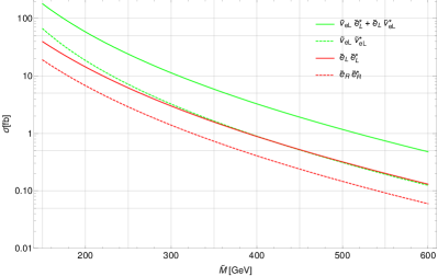
In Figure 1 we present the cross sections for $\tilde{e}_{L,R}$/$\tilde{\nu}_{L}$ production at tree-level. Notice that these cross sections are the same for the $\tilde{\mu}_{L,R}$/$\tilde{\nu}_{\mu L}$ and $\tilde{\tau}_{L,R}$/$\tilde{\nu}_{\tau L}$ flavours. It is well-known that QCD corrections shift these to larger values Fuks:2013vua , so we apply an overall K-factor of 1.17. Note that the sum of the processes $pp\to\tilde{e}_{L}\tilde{\nu}_{eL}^{*}$ and $pp\to\tilde{e}_{L}^{*}\tilde{\nu}_{eL}$ has by far the largest cross section, followed by $\tilde{e}_{L}\tilde{e}_{L}^{*}$ and $\tilde{\nu}_{eL}\tilde{\nu}_{eL}^{*}$ pair production. In the following, we focus on the resulting signal from the decay of these states, as they explain the main features of our results. Nevertheless, in the numerical analysis we have included all possible processes, such that the available data is fully exploited.

Note that left-right mixing in the stau sector is large, such that both $\tilde{\tau}^{-}_{1}$ and $\tilde{\tau}^{-}_{2}$ have a relatively large $\tilde{\tau}^{-}_{L}$ component. This means that in the following we need to study the decays of both states.

The final states, and thus the signal, depend on the nature of the LSP, which can be either an R-sneutrino or a neutralino. Moreover, in case of an R-sneutrino LSP, we also have a different phenomenology depending on wheth-er the higgsinos are lighter or heavier than the L-sleptons. In addition, in the case of higgsinos being lighter than the L-sleptons, we shall also have a dependence on the size of the small gaugino admixture to the physical charginos and neutralinos.

Before we give details of each scenario, we first review the relevant part of the interaction Lagrangian of $\tilde{l}_{L}$ and $\tilde{l}_{R}$ with charginos and neutralinos:

$${\cal L}=\sum_{\begin{subarray}{c}i=1,\dots,4\\ j=L,R\end{subarray}}\big{(} \bar{l}(c^{L}_{ij\tilde{l}}P_{L}+c^{R}_{ij\tilde{l}}P_{R})\tilde{\chi}^{0}_{i}\tilde{l}_{j}$$

$$+\bar{\nu}(c^{L}_{ij\tilde{\nu}}P_{L}+c^{R}_{ij\tilde{\nu}}P_{R})\tilde{\chi}^{0}_{i}\tilde{\nu}_{j}+h.c.\big{)}$$

$$+\sum_{\begin{subarray}{c}k=1,2\\ j=L,R\end{subarray}}\big{(} (\bar{\nu}_{R}d^{L}_{kj\tilde{l}}P_{L}+\bar{\nu}_{L}d^{R}_{kj\tilde{l}}P_{R})\tilde{\chi}^{+}_{k}\tilde{l}_{j}$$

$$+\left(\bar{l}_{R}d^{L}_{kj\tilde{\nu}}P_{L}+\bar{l}_{L}d^{R}_{kj\tilde{\nu}}P_{R}\right)\tilde{\chi}^{+}_{k}\tilde{\nu}_{j}+h.c.\big{)}$$ (2.5)

with

$$c^{L}_{iL\tilde{l}} =-Y_{l}N_{i3}^{*} c^{R}_{iL\tilde{l}} =\frac{1}{\sqrt{2}}\left(g^{\prime}N_{i1}+gN_{i2}\right)$$ (2.6)

$$c^{L}_{iR\tilde{l}} =-\sqrt{2}g^{\prime}N_{i1}^{*} c^{R}_{iR\tilde{l}} =-Y_{l}N_{i3}$$ (2.7)

$$c^{L}_{iL\tilde{\nu}} =-Y_{\nu}N_{i4}^{*} c^{R}_{iL\tilde{\nu}} =\frac{1}{\sqrt{2}}\left(g^{\prime}N_{i1}-gN_{i2}\right)$$ (2.8)

$$c^{L}_{iR\tilde{\nu}} =0 c^{R}_{iR\tilde{\nu}} =-Y_{\nu}N_{i4}$$ (2.9)

$$d^{L}_{kL\tilde{l}} =Y_{\nu}V_{k2}^{*} d^{R}_{kL\tilde{l}} =-gU_{k1}$$ (2.10)

$$d^{L}_{kR\tilde{l}} =0 d^{R}_{kR\tilde{l}} =Y_{l}U_{k2}$$ (2.11)

$$d^{L}_{kL\tilde{\nu}} =Y_{l}U_{k2}^{*} d^{R}_{kL\tilde{\nu}} =-gV_{k1}$$ (2.12)

$$d^{L}_{kR\tilde{\nu}} =0 d^{R}_{kR\tilde{\nu}} =Y_{\nu}V_{k2}$$ (2.13)

where, for simplicity, we have neglected generation indices as well as left-right mixing. This is a very good approximation for the sneutrinos, the first two slepton generations, and for the staus in case of small to medium values of $\tan\beta$.

The neutralino mixing matrix $N$ is in the basis $\tilde{b}$, $\tilde{w}^{3}$, $\tilde{H}_{d}$, $\tilde{H}_{u}$, and in our model we have $|N_{i1}|,|N_{i2}|\ll|N_{i3}|,|N_{i4}|$, for $i=1,2$. Moreover, $U$ and $V$ are the chargi-no mixing matrices, in the basis $\tilde{w}^{\pm},\tilde{H}^{\pm}$, such that in our model we have $|U_{11}|,|V_{11}|\ll|U_{12}|,|V_{12}|$. In addition, we know that $Y_{l},Y_{\nu}\ll g^{\prime},g$, the only exception being $Y_{\tau}$, which can become $\mathcal{O}\left({g^{\prime}}\right)$ in case of very large $\tan\beta$.

Knowing these couplings is very convenient at the time of understanding the different branching ratios. For example, if we want to compare the $\tilde{\mu}_{L}$ decays into higgsinos, for very large values of $M_{1}$, $M_{2}$, we find:

$$\frac{{\rm BR}(\tilde{\mu}_{L}^{-}\to\nu_{L}\tilde{\chi}^{-}_{k})}{{\rm BR}(\tilde{\mu}_{L}^{-}\to\mu^{-}\tilde{\chi}^{0}_{i})}\sim\frac{|g\,U_{k1}|^{2}}{|Y_{\mu}N_{i3}|^{2}}$$ (2.14)

where we see that decays into charginos will be subdominant if the mixing with gauginos is small enough.

2.1 Sneutrino LSP and light higgsinos ($m_{\tilde{\nu}_{R}}<\mu<m_{\tilde{L}}$)

This scenario is characterized by subsequent two-body decays. The heavier L-sleptons decay into states involving $\tilde{\chi}^{0}_{1,2}$ or $\tilde{\chi}^{\pm}_{1}$, which then decay into states involving R-sneutrinos. The decay chains have several branches, with the dominant branching ratio for L-sleptons depending on the size of the couplings and the respective elements of neutralino and chargino mixing matrices.

In the following, for each slepton, we compare two scenarios. In the first one, we set $M_{1}=M_{2}=2$ TeV, such that there is a small but non-negligible gaugino admixture on the neutralino and chargino states. On the second one, both gauginos are “decoupled” from the model by setting their masses at 1 PeV.

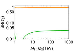
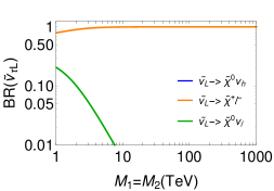
For definiteness, we shall set $m_{\tilde{L}}=600~{}{\rm GeV}$, $\mu=120$ GeV and $\tan\beta=6$. In Figure 2, we show the most important branching ratios of each slepton as a function of $M_{1}=M_{2}$, which shall now be discussed. Notice we neglect to comment those cases where two contributions interfere destructively, as this effect is not of our interest.

Figure 2: Branching ratios for sleptons as a function of gaugino mass $M_{1}=M_{2}$, for $\mu<m_{\tilde{L}}$ Decays for charged sleptons (sneutrinos) are shown on the left (right) column. The last panels describe the colours for the branching ratios shown in each column. In case of neutralinos, the sum over the two lightest states is shown.

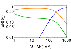
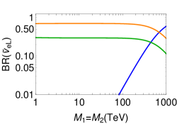
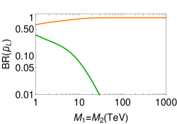
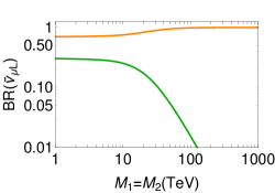
For the smuon $\tilde{\mu}_{L}^{-}$, the 2 TeV gaugino scenario leads to primarily $\tilde{\mu}^{-}_{L}\to\mu^{-}\tilde{\chi}^{0}$ ($75\%$), followed by $\tilde{\mu}^{-}_{L}\to\nu_{L}\tilde{\chi}^{-}$ ($25\%$). The latter decay is due to a gauge coupling, and its branching ratio vanishes when the gauginos decouple. In contrast, $\tilde{\mu}^{-}_{L}\to\mu^{-}\tilde{\chi}^{0}$ is due to a combination of $Y_{\mu}$ and gauge contributions, and its branching ratio rises to unity in the decoupling regime. The muon sneutrino $\tilde{\nu}_{\mu L}$ follows a very similar pattern, with $\tilde{\nu}_{\mu L}\to\mu^{-}\tilde{\chi}^{+}$ dominating ($70\%$ at 2 TeV, and then $100\%$ in the decoupling scenario), followed by $\tilde{\nu}_{\mu L}\to\nu_{L}\tilde{\chi}^{0}$, which decreases in front of rising gaugino masses.

The case for the selectron $\tilde{e}_{L}^{-}$ is very similar to the one for $\tilde{\mu}_{L}^{-}$ in the 2 TeV case, replacing $\mu$ by $e$, and with very similar branching ratios. However, in the gaugino decoupling scenario, we find that the most relevant decay is $\tilde{e}_{L}^{-}\to\nu_{h}\tilde{\chi}^{-}$ ($90\%$), followed by $\tilde{e}_{L}^{-}\to e^{-}\tilde{\chi}^{0}$ ($9\%$) and $\tilde{e}_{L}^{-}\to\nu_{L}\tilde{\chi}^{-}$ ($1\%$). The reason for this is that the first decay proceeds through a $Y_{\nu}$ coupling, which is larger than the $Y_{e}$ coupling that governs the second decay. Again, the electron sneutrino $\tilde{\nu}_{eL}$ decays are similar to the $\tilde{\nu}_{\mu L}$ for 2 TeV gauginos, and in the decoupling case they change to $\tilde{\nu}_{eL}\to\nu_{h}\tilde{\chi}^{0}$ ($60\%$), $\tilde{\nu}_{eL}\to e^{-}\tilde{\chi}^{+}$ ($30\%$) and $\tilde{\nu}_{eL}\to\nu_{L}\tilde{\chi}^{0}$ ($10\%$).

Stau decays are somewhat unique, as the mass eigenstates have large components of both $\tilde{\tau}_{L}^{-}$ and $\tilde{\tau}_{R}^{-}$. We find that the lightest stau, $\tilde{\tau}_{1}^{-}$, which is mostly $\tilde{\tau}_{R}^{-}$, decays in equal proportions through $\tilde{\tau}_{1}^{-}\to\tau^{-}\tilde{\chi}^{0}$ and $\tilde{\tau}^{-}_{1}\to\nu_{L}\tilde{\chi}^{-}$ ($50\%$). In contrast, the heaviest stau, mainly $\tilde{\tau}_{L}$, decays through $\tilde{\tau}^{-}_{2}\to\tau^{-}\tilde{\chi}^{0}$ ($97\%$) and $\tilde{\tau}^{-}_{2}\to\nu_{L}\tilde{\chi}^{+}$ ($3\%$). Ignoring interference effects, the branching ratios of both $\tilde{\tau}_{1}$ and $\tilde{\tau}_{2}$ are independent of the mass of the gauginos. The reason for this is that the stau states can always couple with higgsinos through the $Y_{\tau}$ coupling, which is relatively large. For $\tilde{\tau}_{2}$, the difference in the values of the branching ratios is due to $\tilde{\tau}_{2}^{-}\to\nu_{L}\tilde{\chi}^{+}$ being somewhat suppressed due to the need of $LR$ mixing.

The tau sneutrino $\tilde{\nu}_{\tau L}$ follows a different pattern, as here there is no large mixing with any $\tilde{\nu}_{R}$, such that gaugino couplings can play an important role again. For the 2 TeV gaugino scenario, the dominating decay is $\tilde{\nu}_{\tau L}\to\tau^{-}\tilde{\chi}^{+}$ ($90\%$), followed by $\tilde{\nu}_{\tau L}\to\nu_{L}\tilde{\chi}^{0}$ ($10\%$). The former increases to ($100\%$) in the decoupled case, as in the $\tilde{\nu}_{\mu L}$ scenario.

In all scenarios, the charginos decay into a charged lepton, and a light sneutrino: $\tilde{\chi}^{-}_{1}\to\ell^{-}\tilde{\nu}_{1,2,3}$. The charged lepton is usually a muon or a tau, due to the $Z^{\rm NH}_{a}$ factors in the Yukawa couplings, Eqs (2.3), with the branching ratio into an electron being below 10%. Moreover, due to their couplings, the branching ratio of the decay into $\tilde{\nu}_{1}$ is very suppressed, so charginos decay mostly into $\tilde{\nu}_{2,3}$. In principle, these should decay further through 3-body processes into additional leptons and $\tilde{\nu}_{1}$. However, we find $\tilde{\nu}_{2,3}$ to be long-lived, and escape the detector. Thus, charginos contribute to our signal with a charged lepton and missing energy. Neutralinos follow a similar trend, but decay into a light neutrino instead of a charged lepton. Thus, neutralinos can be considered missing energy.

Finally, one has to take into account the decays of the heavy neutrinos, which are independent of the SUSY scenario considered. The heaviest neutrinos form a pseudo-Dirac pair, and shall decay promptly Atre:2009rg . We shall concentrate on decays involving at least one charged lepton: $\nu_{5,6}\to\ell^{-}qq^{\prime}$ or $\nu_{5,6}\to\ell^{-(\prime)}\ell^{+}\nu_{\ell}$, with off-shell mediators.

2.2 Sneutrino LSP and heavy higgsinos ($m_{\tilde{\nu}_{R}}<m_{\tilde{L}}<\mu$)

The situation changes drastically once the $\mu$ parameter is larger than the slepton mass. In that case, the previous decays are not possible, and one either needs to consider alternative two-body channels, or new three-body decays. We show the available branching ratios in Figure 3, as a function of the slepton mass, where we have fixed $\mu=400$ GeV.

Figure 3: Branching ratios for sleptons as a function of slepton soft mass $m_{\tilde{L}}$, for $m_{\tilde{L}}<\mu=400$ GeV. Decays for charged sleptons (sneutrinos) are shown on the left (right) column. The last panels describe the colours for the branching ratios shown in each column.

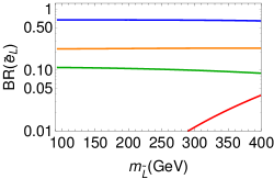
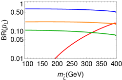
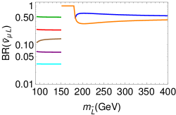
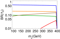
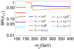
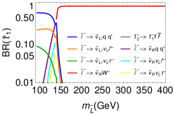
For $\tilde{e}_{L}^{-}$ and $\tilde{\mu}_{L}^{-}$, we find that the dominant decay is $\tilde{\ell}^{-}_{L}\to\tilde{\nu}_{\ell L}W^{-*}$, with the virtual $W^{-}$ giving jet pairs or a charged lepton plus a light neutrino. As usual, decays with quark final states have larger branching ratios.

Another possibility is to decay directly to an R-sneutri-no and a real $W^{-}$ ($\tilde{\ell}^{-}_{L}\to\tilde{\nu}_{2,3}W^{-}$). This process depends on the small $LR$ mixing in the sneutrino sector, so it is proportional to $Y_{\nu}$. We find that the branching ratio for $\tilde{\mu}_{L}^{-}$ is generally smaller than $20\%$. As mentioned earlier, the $Z_{e}^{\rm NH}$ factor in $Y_{\nu}$ is slightly suppressed with respect to $Z_{\mu}^{\rm NH}$, so for $\tilde{e}_{L}^{-}$ the branching ratio is smaller.

The stau sector has a slightly different phenomenology, due to the large left-right mixing. In particular, this leads the predictions of this scenario to depend strongly on $\tan\beta$. The mixing splits the states, such that $\tilde{\tau}_{2}^{-}\to\tilde{\tau}_{1}^{-}Z^{0*}$ decay is allowed. The inclusion of this new channel modifies the other $\tilde{\nu}_{\tau L}\,W^{-*}$ and $\tilde{\nu}_{2,3}\,W^{-}$ branching ratios.

The $\tilde{\tau}_{1}^{-}$, on the other hand, for small $m_{\tilde{L}}$, has similar $\tilde{\nu}_{\tau L}W^{-*}$ decays, with non negligible $\tilde{\nu}_{R}W^{-*}$ contributions. The reason for this is that the mixing-induced mass shift implies that $\tilde{\tau}_{1}^{-}$ is close in mass to the $\tilde{\nu}_{\tau L}$, leading to a strong kinematical suppression. As a consequence the two-body decay into $\tilde{\nu}_{R}\,W^{-}$ clearly dominates once kinematically allowed, despite the fact that there is only a small left-right mixing in the sneutrino sector. Thus, with the exception of $\tilde{\tau}_{1}^{-}$, charged slepton decay shall usually produce one additional $\tilde{\nu}_{\ell L}$. These states shall be accompanied by jets more than $50\%$ of the time.

We find that all $\tilde{\nu}_{L}$ flavours have the same behaviour. For low masses, the decays are governed by off-shell $Z^{0}$- and $h^{0}$-boson exchange, and a $\tilde{\nu}_{R}$ emission. For larger masses, the branching ratios are dominated by two-body decays into a $\tilde{\nu}_{R}$ and an on-shell $Z^{0}$ or $h^{0}$ boson, if kinematically allowed. When both bosons are accessible, the decays into the light Higgs have larger branching ratios.

2.3 Higgsino LSP ($\mu<m_{\tilde{\nu}_{R}}$)

For completeness, we also study the case where the higgsino is the LSP. This is motivated by the fact that it has not been considered so far in the literature.

In this scenario the sleptons and sneutrinos have two-body decays only as described above for the case of $M_{1}=M_{2}=2~{}{\rm TeV}$. We note that, at the one-loop level, a mass splitting between the lightest neutralino and the chargino is induced via the photon-loop yielding the contribution Barducci:2015ffa

$$\Delta m_{\tilde{\chi}^{+}}=\frac{|\mu|\alpha(m_{Z})}{\pi}\left(2+\log\left(\frac{|\mu|^{2}}{m^{2}_{Z}}\right)\right)$$ (2.15)

This implies that the chargino will always have a sufficiently large decay width such that it decays inside the detector. However, due to the small mass differences, the decay products of the lightest chargino and the second heaviest neutralino are so soft that they mainly contribute to the missing transverse momentum. Note that, in this case, $\tilde{\nu}_{i}$ are hardly produced in the decays of the sleptons and heavier L-sneutrinos.

3 Set-up

For this investigation we have used a series of public programs: As a first step we have used SARAH Staub:2008uz ; Staub:2013tta ; Staub:2012pb ; Staub:2010jh ; Staub:2009bi in the SUSY/BSM toolbox 2.0.1 Staub:2011dp ; Staub:2015kfa to implement the model into the event generator MadGraph5_aMC@NLO 2.5.2 Alwall:2014hca . For each set of parameters, we use SPheno 3.3.8 Porod:2003um ; Porod:2011nf to numerically calculate the mass spectrum and branching ratios. After generating the hard scattering in MadGraph, the showering and hadronization is carried out internally with PYTHIA 8.233 Sjostrand:2006za , which uses the CTEQ6L1 PDF set Pumplin:2002vw . We also use PYTHIA for the heavy neutrino decays. As default we generate 25000 events for every production process. The generated events are then fed into CheckMATE 2.0.7 Drees:2013wra ; Dercks:2016npn , which uses Delphes 3.4.0 as detector simulation deFavereau:2013fsa .

Given a specific experimental search, CheckMATE compares the number of events passing each signal region with the observed $S95$ limit obtained by the experiment via the parameter

$$r^{c}=\frac{S-1.64\cdot\Delta S}{S^{95}_{obs}}$$ (3.1)

with $S$ being the number of events in the considered signal region, $\Delta S$ the error from the Monte Carlo and $S^{95}_{obs}$ is the experimentally observed 95% confidence limit on the signal Drees:2013wra ; Drees:2015aeo . In our work, we indicate CheckMATE to compare our predicted signal with all of the available experimental searches.

Notice that Eq. (3.1) does not capture all theoretical uncertainties, such as missing higher order corrections in the production and decays of the various particles. Moreover, there are effects due to variations of the input parameters. For example, in case of an $\tilde{\nu}_{R}$-LSP, the charginos will decay into either a $\mu$ or $\tau$ plus one of the $R$-sneutrinos which escapes detection. The ratio of $\mu$ over $\tau$ depends on $Y_{\nu}$ and varies with the choice of neutrino mixing angles. We therefore follow the basic idea presented in ref. Drees:2015aeo to capture such uncertainties: we do not take the $r^{c}=1$ value as sharp boundary but assume that all points with $r^{c}\geq 1.2$ ($r^{c}\leq 0.8$) are excluded (allowed) whereas for the range in between one would need a more detailed investigation.

For each point, we have also checked that the Z and Higgs invisible width respect experimental bounds, and that the heavy neutrino mixing is small enough to avoid direct detection Deppisch:2015qwa . We have also checked that LFV processes such as $\mu\to e\gamma$, do not exceed the current constraints Abada:2014kba . In this scenario, the SUSY contribution to LFV is very small, either due to the heavy gaugino masses, or due to the small Yukawa couplings. Thus, the non-SUSY part dominates, and as one can see in Gago:2015vma , for the current choice of $M_{5}$, $M_{6}$ and $\gamma_{56}$, it does not saturate the bounds.

4 Results

4.1 Higgsino LSP

We study first the case of a higgsino LSP. In these scenarios the sleptons decay directly into either a lepton and missing energy, or invisibly. The latter case occurs in case of $\tilde{l}\to\nu\tilde{\chi}^{-}$ because the decay products of the charginos are very soft.

For the following investigation we have fixed $M_{1}=M_{2}=1$ TeV implying that (i) the $\tilde{e}$ decays are mainly via the small gaugino admixtures in the chargino and neutralinos and (ii) there will be practically no right-handed neutrinos produced in the slepton decays. From this point of view we are effectively in the usual MSSM with a higgsino LSP. However, to our knowledge the bounds on the slepton mass parameters due to the LHC data have not been presented in the literature.

Figure 4: Constraints on combinations of $m_{\tilde{E}}$ and $m_{\tilde{L}}$ due to slepton/sneutrino production in case of a higgsino LSP with $M_{1}=M_{2}=1$ TeV, $\mu=120$ GeV and $\tan\beta=10$. Red points are excluded, blue ones are allowed and in case of the green ones no conclusive statement can be drawn, within the known theoretical and experimental uncertainties.

In this scenario, the most important analysis is the search for two same sign leptons in combination with large missing transverse energy, carried out in ATLAS:2016uwq . This leads to bounds on the $m_{\tilde{E}}-m_{\tilde{L}}$ plane, which are shown in Figure 4 for the case $\mu=120$ GeV and $\tan\beta=10$. On this Figure, one can see that $m_{\tilde{L}}<400$ GeV is excluded, independent of $m_{\tilde{E}}$. This constraint increases up to 500 GeV if, in addition, light $\tilde{\ell}_{R}^{-}$ are present.

In contrast, even $\tilde{\ell}_{R}$ with a mass of 200 GeV cannot be excluded, which can be seen in the Figure in the limit of heavy $\tilde{\ell}^{-}_{L}$. We understand this is due to insufficient LHC data having been analysed. However, this might change in the near future, once the full 2016 data set has been investigated by ATLAS and CMS.

The structure for $m_{\tilde{L}}\raise 1.29167pt\hbox{$\;>$\kern-7.5pt\raise-4.73611pt\hbox{$\sim\;$}}$ 600 GeV and $m_{\tilde{E}}\raise 1.29167pt\hbox{$\;<$\kern-7.5pt\raise-4.73611pt\hbox{$\sim\;$}}250$ GeV can be understood from the interplay of different signal regions defined in ATLAS:2016uwq . These regions differ mainly in the required bound on the ‘stransverse’ mass $m_{T2}$ Lester:1999tx ; Barr:2003rg : $m_{T2}\geq 90$, 120, 150 GeV, corresponding to the signal regions 2LASF, 2LBSF and 2LCSF, respectively. Taking, for example, $m_{\tilde{L}}=625$ GeV, one finds that for $m_{\tilde{E}}=200$, 225, 250 and 275 GeV, the signal region 2LASF, 2LBSF, 2LBSF and 2LCSF is the most important one, respectively.

Last but not least, we remind that if the mass difference between the sleptons and the higgsinos gets too small, then the average value of the transverse moment of the lepton could be below 20 GeV. This can be a problem, as the $p_{T}$ cut for the leading (subleading) lepton in this search is of 25 GeV (20 GeV). In this situation, one cannot carry out any exclusions, as the final states are not energetic enough to pass the triggers.

Figure 5: $r^{c}$ as a function for $\tan\beta=10$, $M_{1}=M_{2}=1$ TeV and $\mu=120$, 150, 200 and 250 GeV, respectively. The grey band ($0.8\leq r^{c}\leq 1.2$) gives the region where one cannot draw a conclusion whether the point is allowed or not, values below are allowed and those above are excluded.

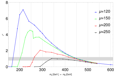
We note that the results hardly depend on the value of $\tan\beta$, whose main effect is to enlarge the mass splitting of the staus for growing values. More important is the size of $\mu$ as this affects the kinematics, e.g. larger values of $|\mu|$ imply softer leptons for fixed slepton mass parameters. This is demonstrated in Fig. 5, where we display the $r^{c}$-value for different values of $\mu$ as a function of $m_{\tilde{L}}=m_{\tilde{E}}$. As we have mentioned previously, scenarios with $r^{c}$ values below 0.8 are allowed, the ones with $r^{c}>1.2$ are excluded whereas for those in between (gray band) no conclusive statement can be made. The structure close to the maxima of the different curves is again due to the interplay of the different signal regions.

4.2 R-Sneutrino LSP

As we have seen in Sections 2.1 and 2.2, on the R-sneutrino LSP scenario, different decays occur depending on the size of $\mu$ with respect to $m_{\tilde{L}}$. Thus, in order to study this situation appropriately, we first need to understand the constraints on chargino pair production.

As mentioned previously, after production, each char-gino decays into a $\tilde{\nu}_{2,3}$ and a charged lepton. Thus, the main constraints arise from the search for two leptons plus missing transverse energy at 13 TeV ATLAS:2016uwq . For very small values of $\mu$, additional constraints arise from the measurement of the $W^{+}W^{-}$ cross section at 8 TeV, with subsequent decays of the $W$ into leptons ATLAS-CONF-2014-033 . In this case, the charginos would contribute more than what is allowed by the experimental uncertainty to the $W^{+}W^{-}$ signal regions.

Figure 6: Constraints on combinations of $m_{\tilde{\nu}_{R}}$ and $\mu$ due to chargino pair production $pp\to\tilde{\chi}^{+}\tilde{\chi}^{-}\to l^{+}l^{-}\tilde{\nu}_{R}\tilde{\nu}_{R}^{*}$. Colour conventions follow Figure 4.

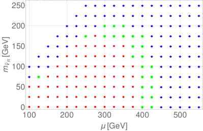
In Figure 6, we show the exclusion region in the $\mu-m_{\tilde{\nu}_{R}}$ parameter space, based on $\tilde{\chi}^{+}\tilde{\chi}^{-}$ production. From the plot, we see that, for vanishing $m_{\tilde{\nu}_{R}}$, the bound on $m_{\tilde{\chi}^{\pm}}$ can be as large as 375 GeV. Note that the $\tilde{\nu}_{2,3}$, for $m_{{\tilde{\nu}}_{R}}=0$, have nearly the same masses as the right-handed neutrinos. For relatively small values of $\mu$, one finds that R-sneutrino masses lighter than $\mu-75$ GeV are ruled out, with the allowed region increasing for $\mu\gtrsim 250$ GeV. For completeness, we note that this exclusion does not depend on the sign of $\mu$ or the value $\tan\beta$.

In Section 2.1, we analyzed two scenarios for the gauginos, one where $M_{1}=M_{2}=2$ TeV, and another “decoupled” scenario, where we set $M_{1}=M_{2}=1$ PeV. Given our results for chargino production, we explore two additional possibilities. On the first one (“varying $\mu$”), we set $\mu=m_{\tilde{\nu}_{R}}+25$ GeV, such that we always have $m_{\tilde{\nu}_{R}}<\mu<m_{\tilde{L}}$. On the second one (“fixed $\mu$”), we set $\mu=400$ GeV, such that one also needs to take into account the $m_{\tilde{\nu}_{R}}<m_{\tilde{L}}<\mu$ case. Thus, four different exclusion plots will be generated. In all of these, we merge exclusions from 8 and 13 TeV data.

Figure 7: Constraints on combinations of $m_{\tilde{\nu}_{R}}$ and $m_{\tilde{L}}$ due to slepton/sneutrino production in case of an R-sneutrino LSP with $M_{1}=M_{2}=2$ TeV ($M_{1}=M_{2}=1$ PeV) on the left (right) panel. We fix $\mu=m_{\tilde{\nu}_{R}}+25$ GeV and $\tan\beta=6$. Colour conventions follow Figure 4.

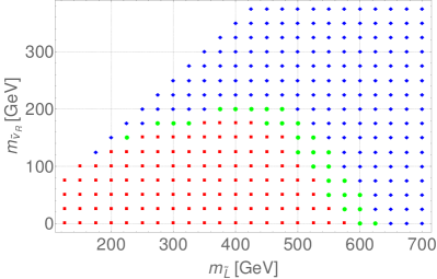
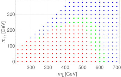
We show the constraints on the varying $\mu$ scenario in Figure 7. Here, the relevant analysis is again ATLAS:2016uwq , which searches for events with 2-3 leptons and missing energy. We find that, for both choices of gaugino mass, we can rule out values of $m_{\tilde{L}}$ as large as 575 GeV. In addition, for lighter slepton masses, it is possible to rule out R-sneutrino masses as heavy as 175-225 GeV, depending on the amount of gaugino admixture.

The exclusion for “decoupled” gauginos is stronger, which can be understood from Figure 2. For $\tilde{\ell}_{L}$, all possible decays shall lead at least to one charged lepton, for all values of gaugino mass (recall that, in this scenario, charginos decay always into final states with visible charged leptons). However, for $\tilde{\nu}_{\ell L}$, one finds that it is possible to have only missing energy on the final state, due to $\tilde{\nu}_{\ell L}\to\nu_{L}\tilde{\chi}^{0}$ decay. This decay channel is suppressed in the “decoupled” scenario, meaning that it is much more likely to have energetic charged leptons on the final state, which strengthens the multi-lepton signal.

Figure 8: Constraints on combinations of $m_{\tilde{\nu}_{R}}$ and $m_{\tilde{L}}$ due to slepton/sneutrino production in case of an R-sneutrino LSP with $M_{1}=M_{2}=2$ TeV ($M_{1}=M_{2}=1$ PeV) on the left (right) panel. We fix $\mu=400$ GeV and $\tan\beta=6$. Colour conventions follow Figure 4.

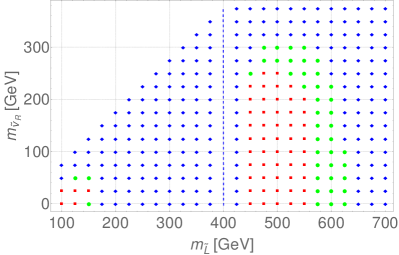
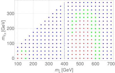
The constraints on the fixed $\mu$ case are shown in Figure 8, again, for different values of gaugino mass. Here it is very interesting to note that there are very weak constraints when $m_{\tilde{L}}<\mu$. The reason for this can be found in Figure 3. We see that in most of the cases, we have the charged slepton decaying into $\tilde{\nu}_{\ell L}$ and light fermions. Given the proximity in the slepton masses, most light fermions end up being very soft, and elude detection. On the other hand, when the two resulting $\tilde{\nu}_{\ell L}$ decay, the decay products shall involve either an on-shell $h^{0}$ or $Z^{0}$. This is again problematic for detection, as fermions coming from these states are generally avoided in new physics searches by suitable cuts to suppress SM background. This leaves us sensitive only to the very low $m_{\tilde{L}}$ region, where L-sneutrino three-body decays are allowed.

For large values of $m_{\tilde{L}}$, we return to the $\mu<m_{\tilde{L}}$ scenario. Here, again, we have ATLAS:2016uwq giving the relevant constraints. The bounds reach $m_{\tilde{L}}$ as large as 575 GeV for vanishing $m_{\tilde{\nu}_{R}}$. Morover, for smaller charged slepton masses, we can bound $m_{\tilde{\nu}_{R}}$ up to 250 GeV. This is all consistent with our results for the varying $\mu$ scenario.

5 Conclusions

In this work, the MSSM was extended by three right-handed neutrino superfields, with active neutrino masses being provided through the seesaw mechanism. In addition, driven by naturalness arguments, the $\mu$ term was kept relatively small, such that the lightest neutralinos were higgsino-like. We considered LHC data on this model, and explored how much existing data constrain such scenarios.

Two possibilities were considered for the nature of the LSP. On the first one, this was a higgsino-like neutralino. In this case, one requires a non-vanishing gaugino admixture in order not to have too long-lived charginos. The sleptons would decay into SM particles and neutralinos. We carried out an analysis considering $m_{\tilde{L}}\neq m_{\tilde{E}}$, for fixed neutralino mass, and found that only $m_{\tilde{L}}$ could be bounded. For $\mu=120$ GeV, we can rule out at least $m_{\tilde{L}}<400$ GeV for all values of $m_{\tilde{E}}$, and $m_{\tilde{L}}<500$ GeV for $m_{\tilde{E}}=200$ GeV.

On the second possibility we considered, the right-handed neutrino superpartner, the R-sneutrino, was taken as the LSP. This provided a very complex scenario, depending on the relative size of the neutralino / chargino mass with respect to the slepton mass. The phenomenology also depended on the amount of gaugino component within the neutralinos. We found that, as long as $\mu<m_{\tilde{L}}$, we can exclude slepton masses to a maximum of $575$ GeV, for vanishing $m_{\tilde{\nu}_{R}}$. For lower values of slepton mass, the R-sneutrino masses can be excluded up to about 200 GeV. In case $m_{\tilde{L}}<\mu$, constraints became very weak, as final states were either too soft, or excluded from signal regions.

Appendix A Parametrization of the Neutrino Sector

In order to parametrize neutrino mixing, we generalize the work in Casas:2001sr ; Donini:2012tt to three heavy neutrinos. The $6\times 6$ neutrino mixing matrix $U$ is decomposed into four $3\times 3$ blocks:

$$U_{6\times 6}=\left(\begin{array}[]{cc}U_{a\ell}&U_{ah}\\ U_{s\ell}&U_{sh}\end{array}\right)~{}.$$ (A.1)

where $a=e,\,\mu,\,\tau$ and $s=s_{1},\,s_{2},\,s_{3}$ make reference to the active and sterile states, while $\ell=1,\,2,\,3$ and $h=4,\,5,\,6$ refer to the light and heavy mass eigenstates, respectively.

For the normal hierarchy, each block can be parame-trized in the following way:

$$U_{a\ell} =U_{\rm PMNS}\,H~{},$$ (A.2)

$$U_{ah} =i\,U_{\rm PMNS}\,H\,m_{\ell}^{1/2}R^{\dagger}M_{h}^{-1/2}~{},$$ (A.3)

$$U_{s\ell} =i\bar{H}M_{h}^{-1/2}\,R\,m_{\ell}^{1/2}~{},$$ (A.4)

$$U_{sh} =\bar{H}~{},$$ (A.5)

where $m_{\ell}={\rm diag}(m_{1},\,m_{2},\,m_{3})$ and $M_{h}={\rm diag}(M_{4},\,M_{5},$ $\,M_{6})$ are $3\times 3$ matrices including the light and heavy neutrino masses, respectively, and:

$$H = \left(I+m_{\ell}^{1/2}\,R^{\dagger}\,M_{h}^{-1}\,R\,m_{\ell}^{1/2}\right)^{-1/2}$$

$$\bar{H} = \left(I+M_{h}^{-1/2}\,R\,m_{\ell}\,R^{\dagger}\,M_{h}^{-1/2}\right)^{-1/2}~{}.$$ (A.6)

In addition, $U_{\rm PMNS}$ corresponds to the standard PMNS matrix in the limit where $H\to I$, and $R$ is a complex orthogonal matrix as in Casas:2001sr , which we parametrize in the following way:

$$R=\left(\begin{array}[]{ccc}1&&\\ &c_{56}&s_{56}\\ &-s_{56}&c_{56}\end{array}\right)\left(\begin{array}[]{ccc}c_{46}&&s_{46}\\ &1&\\ -s_{46}&&c_{46}\end{array}\right)\left(\begin{array}[]{ccc}c_{45}&s_{45}&\\ -s_{45}&c_{45}&\\ &&1\end{array}\right)$$ (A.7)

Here, $s_{ij}$ and $c_{ij}$ are, respectively, the sine and cosine of a complex mixing angle, $\rho_{ij}+i\gamma_{ij}$. With these parameters, one can rebuild the $Y_{\nu}$ and $M_{R}$ matrices, meaning that the neutrino sector is described without ambiguities:

$$Y_{\nu} = -i\frac{\sqrt{2}}{v_{u}}U_{\rm PMNS}^{*}H^{*}m_{\ell}^{1/2}\left(m_{\ell}R^{\dagger}+R^{T}M_{h}\right)M_{h}^{-1/2}\bar{H}$$

$$M_{R} = \bar{H}^{*}M_{h}^{1/2}\left(I-M_{h}^{-1}R^{*}m_{\ell}^{2}R^{\dagger}M_{h}^{-1}\right)M_{h}^{1/2}\bar{H}$$ (A.9)

In general, the active-heavy mixing is suppressed by $(m_{\ell}/M_{h})^{1/2}$, which would imply heavy neutrinos being difficult to probe if their masses are much heavier than those of the light neutrinos. However, this result can be avoided by taking large $\gamma_{ij}$. Since these involve hyperbolic sines and cosines, at least one large $\gamma_{ij}$ would lead to an exponential enhancement of the mixing.

In order to simplify our analysis, in the following we keep $\nu_{4}$ decoupled from $\nu_{5}$ and $\nu_{6}$, setting $\rho_{45}=\rho_{46}=\gamma_{45}=\gamma_{46}=0$, that is, only $\rho_{56}$ and $\gamma_{56}$ are not zero. For GeV masses, and $\gamma_{56}$ in the range $3-10$, we find the standard results:

$$|U_{a4}|^{2} = \left|(U_{\rm PMNS})_{a1}\right|^{2}\frac{m_{1}}{M_{4}}$$ (A.10)

$$|U_{a5}|^{2} = \left|Z^{NH}_{a}\right|^{2}\frac{m_{3}}{M_{5}}\cosh^{2}\gamma_{56}$$ (A.11)

$$|U_{a6}|^{2} = \left|Z^{NH}_{a}\right|^{2}\frac{m_{3}}{M_{6}}\cosh^{2}\gamma_{56}$$ (A.12)

where $Z^{NH}_{a}$ is a factor of $\mathcal{O}\left({1}\right)$ depending on the PMNS mixing angles and the neutrino mass ordering, which can be found in Gago:2015vma . This limit also leads to Eqs. 2.3.

Appendix B Sneutrino Mass Matrix

Being electrically neutral, the sneutrino interaction states can be split into real and imaginary parts:

$$\tilde{\nu}_{L}=\frac{1}{\sqrt{2}}\left(\tilde{\phi}_{LR}+i\tilde{\phi}_{LI}\right) \tilde{\nu}_{R}^{c}=\frac{1}{\sqrt{2}}\left(\tilde{\phi}_{RR}-i\tilde{\phi}_{RI}\right)$$ (B.1)

We can define $\tilde{\phi}_{R}=(\phi_{LR},\,\phi_{RR})^{T}$ and $\tilde{\phi}_{I}=(\phi_{LI},\,\phi_{RI})^{T}$, such that the sneutrino mass term is divided into four $2\times 2$ blocks:

$$\mathcal{L}_{\tilde{\nu}}^{\rm mass}=\frac{1}{2}(\tilde{\phi}_{R}^{T},\,\tilde{\phi}_{I}^{T})\cdot\left(\begin{array}[]{cc}M^{2}_{RR}&M_{RI}^{2}\\ M_{IR}^{2}&M_{II}^{2}\end{array}\right)\cdot\left(\begin{array}[]{c}\tilde{\phi}_{R}\\ \tilde{\phi}_{I}\end{array}\right)$$ (B.2)

The blocks are:

$$M_{RR}^{2}=\left(\begin{array}[]{cc}m_{\tilde{L}}^{2}+\frac{1}{2}m_{Z}^{2}\cos 2\beta+\frac{1}{2}v_{u}^{2}Y_{\nu}Y_{\nu}^{\dagger}&\Re e\left[\frac{v_{u}}{\sqrt{2}}\left(T_{\nu}+Y_{\nu}M_{R}^{\dagger}-\mu^{*}Y_{\nu}\cot\beta\right)\right]\\ \Re e\left[\frac{v_{u}}{\sqrt{2}}\left(T^{T}_{\nu}+M_{R}^{\dagger}Y_{\nu}^{T}-\mu^{*}Y^{T}_{\nu}\cot\beta\right)\right]&m_{\tilde{\nu}_{R}}^{2}+M_{R}^{\dagger}M_{R}+\frac{1}{2}v_{u}^{2}Y_{\nu}^{\dagger}Y_{\nu}+\Re e[B_{\tilde{\nu}}]\end{array}\right)$$ (B.3)

$$M_{II}^{2}=\left(\begin{array}[]{cc}m_{\tilde{L}}^{2}+\frac{1}{2}m_{Z}^{2}\cos 2\beta+\frac{1}{2}v_{u}^{2}Y_{\nu}Y_{\nu}^{\dagger}&\Re e\left[\frac{v_{u}}{\sqrt{2}}\left(T_{\nu}-Y_{\nu}M_{R}^{\dagger}-\mu^{*}Y_{\nu}\cot\beta\right)\right]\\ \Re e\left[\frac{v_{u}}{\sqrt{2}}\left(T^{T}_{\nu}-M_{R}^{\dagger}Y_{\nu}^{T}-\mu^{*}Y^{T}_{\nu}\cot\beta\right)\right]&m_{\tilde{\nu}_{R}}^{2}+M_{R}^{\dagger}M_{R}+\frac{1}{2}v_{u}^{2}Y_{\nu}^{\dagger}Y_{\nu}-\Re e[B_{\tilde{\nu}}]\end{array}\right)$$ (B.4)

$$M_{RI}^{2}=\left(\begin{array}[]{cc}0&\Im m\left[\frac{v_{u}}{\sqrt{2}}\left(T_{\nu}+Y_{\nu}M_{R}^{\dagger}+\mu^{*}Y_{\nu}\cot\beta\right)\right]\\ -\Im m\left[\frac{v_{u}}{\sqrt{2}}\left(T^{T}_{\nu}+M_{R}^{\dagger}Y_{\nu}^{T}-\mu^{*}Y^{T}_{\nu}\cot\beta\right)\right]&-\Im m[B_{\tilde{\nu}}]\end{array}\right)$$ (B.5)

$$M_{IR}^{2}=(M_{RI}^{2})^{T}$$ (B.6)

It is possible to avoid the splitting of $\tilde{\nu}_{L}$ and $\tilde{\nu}_{R}^{c}$ into $\tilde{\phi}_{(L,R)(R,I)}$ if $M^{2}_{RR}=M^{2}_{II}$ and $M^{2}_{RI}=M^{2}_{IR}=0$. This is achieved by taking CP conservation, as well as vanishing $B_{\tilde{\nu}}$ and $Y_{\nu}M_{R}^{\dagger}$. In this work, we have real $\mu$ and $T_{\nu}$, and very small $Y_{\nu}M_{R}^{\dagger}$ and $B_{\tilde{\nu}}$. Thus, to a very good approximation, we can assume that the real and imaginary parts of each field are aligned, so we can work directly with $\tilde{\nu}_{L}$ and $\tilde{\nu}_{R}^{c}$.

References

- (1) G. Aad, et al. (ATLAS), Phys. Lett. B716, 1 (2012), 1207.7214
- (2) S. Chatrchyan, et al. (CMS), Phys. Lett. B716, 30 (2012), 1207.7235
- (3) G. Aad, et al. (ATLAS, CMS), Phys. Rev. Lett. 114, 191803 (2015), 1503.07589
- (4) C. Brust, A. Katz, S. Lawrence, et al., JHEP 03, 103 (2012), 1110.6670
- (5) M. Papucci, J. T. Ruderman, A. Weiler, JHEP 09, 035 (2012), 1110.6926
- (6) L. J. Hall, D. Pinner, J. T. Ruderman, JHEP 04, 131 (2012), 1112.2703
- (7) K. Blum, R. T. D’Agnolo, J. Fan, JHEP 01, 057 (2013), 1206.5303
- (8) J. R. Espinosa, C. Grojean, V. Sanz, et al., JHEP 12, 077 (2012), 1207.7355
- (9) R. T. D’Agnolo, E. Kuflik, M. Zanetti, JHEP 03, 043 (2013), 1212.1165
- (10) H. Baer, V. Barger, P. Huang, et al., JHEP 05, 109 (2012), 1203.5539
- (11) J. E. Younkin, S. P. Martin, Phys. Rev. D85, 055028 (2012), 1201.2989
- (12) G. D. Kribs, A. Martin, A. Menon, Phys. Rev. D88, 035025 (2013), 1305.1313
- (13) E. Hardy, JHEP 10, 133 (2013), 1306.1534
- (14) K. Kowalska, E. M. Sessolo, Phys. Rev. D88, 7, 075001 (2013), 1307.5790
- (15) C. Han, K.-i. Hikasa, L. Wu, et al., JHEP 10, 216 (2013), 1308.5307
- (16) P. Minkowski, Phys. Lett. B67, 421 (1977)
- (17) T. Yanagida, Conf.Proc. C7902131, 95 (1979)
- (18) R. N. Mohapatra, G. Senjanovic, Phys. Rev. Lett. 44, 912 (1980)
- (19) M. Gell-Mann, P. Ramond, R. Slansky, Conf. Proc. C790927, 315 (1979), %****␣Rsneutrino.bbl␣Line␣75␣****1306.4669
- (20) J. Schechter, J. W. F. Valle, Phys. Rev. D22, 2227 (1980)
- (21) R. Foot, H. Lew, X. He, et al., Z.Phys. C44, 441 (1989)
- (22) R. N. Mohapatra, J. W. F. Valle, Phys. Rev. D34, 1642 (1986)
- (23) S. Dodelson, L. M. Widrow, Phys. Rev. Lett. 72, 17 (1994), hep-ph/9303287
- (24) E. K. Akhmedov, V. A. Rubakov, A. Yu. Smirnov, Phys. Rev. Lett. 81, 1359 (1998), hep-ph/9803255
- (25) T. Asaka, M. Shaposhnikov, Phys. Lett. B620, 17 (2005), hep-ph/0505013
- (26) L. M. Carpenter (2016), 1612.09255
- (27) H. Baer, V. Barger, J. S. Gainer, et al. (2017), 1702.06588
- (28) F. Deppisch, J. W. F. Valle, Phys. Rev. D72, 036001 (2005), hep-ph/0406040
- (29) F. Bazzocchi, D. G. Cerdeno, C. Munoz, et al., Phys. Rev. D81, 051701 (2010), 0907.1262
- (30) M. Hirsch, T. Kernreiter, J. C. Romao, et al., JHEP 01, 103 (2010), 0910.2435
- (31) J. A. Casas, A. Ibarra, Nucl. Phys. B618, 171 (2001), hep-ph/0103065
- (32) A. Donini, P. Hernandez, J. Lopez-Pavon, et al., JHEP 1207, 161 (2012), 1205.5230
- (33) A. M. Gago, P. Hernández, J. Jones-Pérez, et al., Eur. Phys. J. C75, 10, 470 (2015), 1505.05880
- (34) D. Barducci, A. Belyaev, A. K. M. Bharucha, et al., JHEP 07, 066 (2015), 1504.02472
- (35) B. Fuks, M. Klasen, D. R. Lamprea, et al., Eur. Phys. J. C73, 2480 (2013), 1304.0790
- (36) A. Atre, T. Han, S. Pascoli, et al., JHEP 0905, 030 (2009), 0901.3589
- (37) F. Staub (2008), 0806.0538
- (38) F. Staub, Comput. Phys. Commun. 185, 1773 (2014), 1309.7223
- (39) F. Staub, Comput. Phys. Commun. 184, 1792 (2013), 1207.0906
- (40) F. Staub, Comput. Phys. Commun. 182, 808 (2011), 1002.0840
- (41) F. Staub, Comput. Phys. Commun. 181, 1077 (2010), 0909.2863
- (42) F. Staub, T. Ohl, W. Porod, et al., Comput. Phys. Commun. 183, 2165 (2012), 1109.5147
- (43) F. Staub, Adv. High Energy Phys. 2015, 840780 (2015), 1503.04200
- (44) J. Alwall, R. Frederix, S. Frixione, et al., JHEP 07, 079 (2014), 1405.0301
- (45) W. Porod, Comput. Phys. Commun. 153, 275 (2003), hep-ph/0301101
- (46) W. Porod, F. Staub, Comput. Phys. Commun. 183, 2458 (2012), 1104.1573
- (47) T. Sjostrand, S. Mrenna, P. Z. Skands, JHEP 05, 026 (2006), hep-ph/0603175
- (48) J. Pumplin, D. R. Stump, J. Huston, et al., JHEP 07, 012 (2002), hep-ph/0201195
- (49) M. Drees, H. Dreiner, D. Schmeier, et al., Comput. Phys. Commun. 187, 227 (2014), 1312.2591
- (50) D. Dercks, N. Desai, J. S. Kim, et al. (2016), 1611.09856
- (51) J. de Favereau, C. Delaere, P. Demin, et al. (DELPHES 3), JHEP 02, 057 (2014), 1307.6346
- (52) M. Drees, J. S. Kim (2015), 1511.04461
- (53) F. F. Deppisch, P. S. Bhupal Dev, A. Pilaftsis, New J. Phys. 17, 7, 075019 (2015), 1502.06541
- (54) A. Abada, M. E. Krauss, W. Porod, et al., JHEP 11, 048 (2014), 1408.0138
- (55) The ATLAS collaboration (ATLAS-CONF-2016-096) (2016), URL http://cds.cern.ch/record/2212162
- (56) C. G. Lester, D. J. Summers, Phys. Lett. B463, 99 (1999), hep-ph/9906349
- (57) A. Barr, C. Lester, P. Stephens, J. Phys. G29, 2343 (2003), hep-ph/0304226
- (58) The ATLAS collaboration (ATLAS-CONF-2014-033) (2014), URL http://cds.cern.ch/record/1728248