CheckMATE: Confronting your Favourite New Physics Model with LHC Data
Abstract
In the first three years of running, the LHC has delivered a wealth of new data that is now being analysed. With over 20 fb-1 of integrated luminosity, both ATLAS and CMS have performed many searches for new physics that theorists are eager to test their model against. However, tuning the detector simulations, understanding the particular analysis details and interpreting the results can be a tedious task.
Checkmate (Check Models At Terascale Energies) is a program package which accepts simulated event files
in many formats for
any model. The program then determines whether the model is excluded or not at 95 C.L.
by comparing to many recent
experimental analyses. Furthermore
the program can calculate confidence limits and provide detailed information about
signal regions of interest. It is simple to use and the program structure allows for
easy extensions to upcoming LHC results in the future.
Checkmate can be found at: http://checkmate.hepforge.org
![[Uncaptioned image]](/html/1312.2591/assets/images/Final.png)
Important Note
-
•
Checkmate is built upon the tools and hard work of many people. If Checkmate is used in your publication it is extremely important that all of the following citations are included,
-
–
Delphes 3 deFavereau:2013fsa .
-
–
FastJet Cacciari:2011ma ; Cacciari:2005hq .
-
–
Anti-kt jet algorithm Cacciari:2008gp .
-
–
CL prescription 0954-3899-28-10-313 .
-
–
In analyses that use the MT2 kinematical discriminant we use the Oxbridge Kinetics Library Lester:1999tx ; Barr:2003rg and the algorithm developed by Cheng and Han Cheng:2008hk .
-
–
All experimental analyses that were used to set limits in the study.
-
–
The Monte Carlo event generator that was used.
-
–
I Introduction
I.1 Motivation
In the three years that the Large Hadron Collider (LHC) has been running, the Beyond the Standard Model (BSM) landscape has changed enormously. To take just a few examples, the possible parameter spaces of Supersymmetry (SUSY) Haber:1984rc ; Nilles:1983ge , Technicolour Weinberg:1975gm ; Susskind:1978ms and Extra Dimensional models ArkaniHamed:1998rs ; Randall:1999ee are now significantly more limited and constrained than in the pre–LHC era.
LHC experimentalists typically classify analyses in terms of a specific final state configuration. They interpret the results in essentially two different approaches: The first strategy is to take a constrained version of a complete model, with a small number of free parameters and investigate exactly what set of model parameters have been excluded by the latest data and which are still allowed. The advantage of such a complete model is its predictivity and the small number of input parameters. However, as soon as the model is slightly modified, it can be very difficult, if not impossible, to set a new appropriate limit. Therefore, only a small number of models tested by the experimental collaborations can be reliably checked.
The second approach employed to great effect at the LHC uses simplified models Alves:2011wf . The idea here is that an effective Lagrangian with only a small number of particles and interactions is considered. Limits on the mass of BSM particles, in particular production and decay topologies, are presented. The production and decay modes chosen are those that often occur in a particular class of models and consequently can be applied widely.
However, the particular interpretation of these results can lead to very different results. For example, the headline limits are often presented in terms of 100% branching ratios and in models with a dark matter candidate Bertone:2004pz , this is often taken as being massless. In most ‘realistic’ models, neither of these assumptions is true which can lead to a far more conservative bound.
One may nevertheless attempt to map the particular model of interest onto the simplified model by considering the rate of events that have exactly the same production and decay topologies. However, rarely are branching ratios 100% and many different production modes may contribute. These different topologies may not be identical to those given in the simplified model and so cannot be safely used to set a limit. Despite this, it is inevitable that some events from these processes will contribute to signal regions. Consequently, the limit set may be far weaker than if the full model had been properly analysed by the particular experimental collaboration.
The above two issues lead to the obvious question of how to reinterpret the data to place bounds on the BSM models that have not previously been analysed by the experiments. Unavoidably, the only way to do this accurately is to generate simulated events and then run these through an implementation of the experimental analysis, including all detector effects. Checkmate is meant to provide the best possible reproduction of both the analysis and detector effects. In addition we aim to simplify and improve confidence in the second step so that any user can investigate the model of their choice.
The idea behind Checkmate is that the user only has to provide event file(s) and the corresponding cross section(s). The user also selects the analyses111If the particular analysis of interest is missing from the current Checkmate list, we welcome requests for new analyses. Indeed, the analysis under question may be almost ready for public release and is only awaiting final validation. against which the event files should be tested. Checkmate then informs the user whether the particular model is excluded or not using the 95% CL 0954-3899-28-10-313 method. In addition, the actual exclusion likelihood can be given if desired.
I.2 Overview
To run Checkmate, the user has to provide simulated event files (in HepMC Dobbs:2001ck or HepEvt Knowles:1995kj ) from an event generator of choice (Pythia Sjostrand:2006za ; Sjostrand:2007gs , Herwig++ Bahr:2008pv , CalcHEPBelyaev:2012qa , MadGraph Alwall:2011uj , Sherpa Gleisberg:2008ta , …) plus the effective cross sections that correspond to these events, e.g. taking into account potential phase space cuts or branching ratios. The total systematic error on the cross section has to be provided which enters the calculation of the total uncertainty. Input events can be weighted and these weights are properly taken into account by Checkmate.
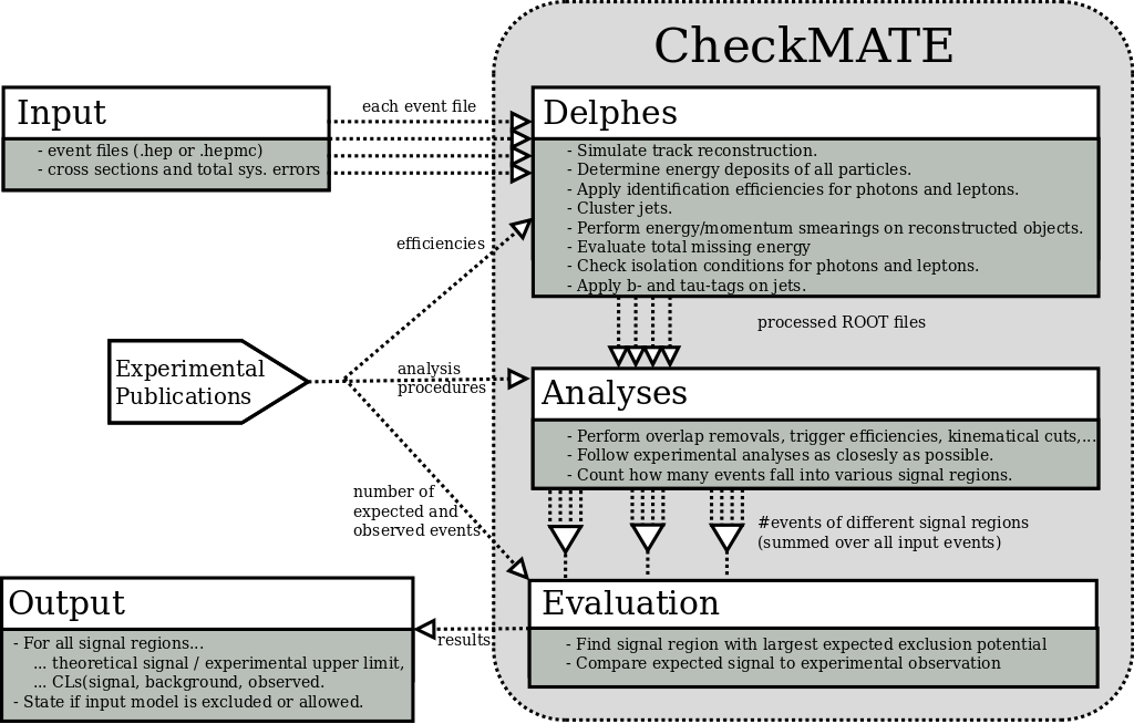
This information is then consecutively processed by three independent modules (see Figure 1). As a first step, the events are run through a fast detector simulation. We have chosen to use Delphes deFavereau:2013fsa , which we have heavily modified to accurately model the ATLAS detector and the final state reconstructions that are performed. This includes the smearing of the visible particles’ momenta according to the respective experimental resolution, efficiency–based object identification, b–/–tagging for jets and reconstruction of the missing transverse momentum vector. The program has been optimised to check for all the final state information needed by the given selection of analyses and to minimise the computational effort by removing redundant and/or superfluous parts from the simulation, see Section III.2 for more details. The results of this simulation are stored in Root trees, which can optionally be read and/or manipulated by the user externally Brun:1997pa .
These files are automatically processed by those of the supplied analyses the user selects when starting Checkmate. A list of currently implemented analyses can be found in Table 1 and will be significantly extended in the coming months. They are internally coded in a well–structured framework that allows for an easy extension to new upcoming experimental results (see Appendix B for more details). It furthermore allows users to easily update given analyses or implement their own.
The input data is processed event by event by checking isolation criteria, removing overlapping objects, and implementing the cuts that define the signal regions. The analysis program determines how many events in total satisfy certain signal region criteria and stores this information in human–readable output for each separate input event file. Both the true number of Monte Carlo events as well as the number of events normalised to the given cross section and luminosity are stored.
The final step of the program consists of a statistical evaluation of the result. For each individual signal region of the chosen analyses, the total number of expected signal events is determined by summing up the results from each input event file. The total uncertainty on this number is determined from both the statistical uncertainty, given by the number of Monte Carlo events, and the systematic uncertainty, which is estimated from the total uncertainty on the signal cross section given by the user. These numbers are compared to the results from the respective experimental search, listed in the references shown in Table 1. There are two possible ways of comparison:
-
1.
Many experimental searches translate their results into model independent 95% upper confidence limits on the number of signal events coming from new physics. A quick–and–easy way of comparison is given by computing the parameter,
(1) In that case, a model can be considered as excluded to the 95% confidence level, if .
-
2.
The user can ask for the explicit confidence level for the given signal. Following common use of experimental searches, Checkmate uses a profile log–likelihood ratio test paired with the CL prescription 0954-3899-28-10-313 to determine the confidence level that corresponds to the determined number of signal events and the expected and observed number of events at the experiment. Both the uncertainty on the signal and on the background are taken into account as Gaussian probability distribution functions around the nominal values. The calculation of the CL allows for Checkmate to be easily included into a fitting routine for the chosen model.
The aforementioned parameters are determined for all signal regions of all selected analyses. If available from the experimental papers, not only the observed but also the expected limits are used. The signal region with the strongest expected limit is determined and the corresponding observed limit is used to state whether the input can be considered excluded or not.
| Internal name | #SR | Description | Ref | CR? | ||
|---|---|---|---|---|---|---|
| atlas_1308_2631 | 2 | 2 b-jets + | 8 TeV | 20.1 fb-1 | Aad:2013ija | |
| atlas_conf_2012_104 | 2 | 1 lepton + 4 jets + | 8 TeV | 5.8 fb-1 | ATLAS-CONF-2012-104 | |
| atlas_conf_2012_147 | 4 | Monojet + | 8 TeV | 10.5 fb-1 | ATLAS-CONF-2012-147 | |
| atlas_conf_2013_024 | 3 | 0 lepton + 6 (2 b-)jets + | 8 TeV | 20.5 fb-1 | ATLAS-CONF-2013-024 | |
| atlas_conf_2013_035 | 6 | 3 leptons + | 8 TeV | 20.7 fb-1 | ATLAS-CONF-2013-035 | |
| atlas_conf_2013_047 | 9 | 0 leptons + 2-6 jets + | 8 TeV | 20.3 fb-1 | ATLAS-CONF-2013-047 | |
| atlas_conf_2013_049 | 9 | 2 leptons + | 8 TeV | 20.3 fb-1 | ATLAS-CONF-2013-049 | |
| atlas_conf_2013_061 | 9 | 0-1 leptons + 3 b-jets + | 8 TeV | 20.1 fb-1 | ATLAS-CONF-2013-061 | |
| atlas_conf_2013_062 | 19 | 1-2 leptons + 3-6 jets + | 8 TeV | 20.3 fb-1 | ATLAS-CONF-2013-062 | |
| atlas_conf_2013_089 | 12 | 2 leptons + jets + | 8 TeV | 20.3 fb-1 | ATLAS-CONF-2013-089 | |
| cms_pas_exo_12_048 | 7 | Monojet | 8 TeV | 19.5 fb-1 | CMS-PAS-EXO-12-048 | |
| cms_1303_2985 | 59 | + b jet multiplicity | 8 TeV | 11.7 fb-1 | Chatrchyan:2013lya |
II Using Checkmate
This section introduces the basic setup of the program. It should give the users enough insight into the program to run the code for their own purposes, which does not require knowledge of the internal details. These will be introduced in Section III.2 and the Appendices. An even simpler version showing the minimum required information to run Checkmate and extract the relevant results is given on the Checkmate website. Checkmate can easily be downloaded and installed222If you encounter problems during installation, please contact us via the webpage and we are happy to help. by the following set of commands:
wget http://www.hepforge.org/archive/checkmate/CheckMATE-Current.tar.gz tar -xvf CheckMATE-Current.tar.gz cd CheckMATE-X.Y.Z ./configure makeMore information on Root prerequisites and installation parameters can be
found in Appendix A. A successful installation should
have created a CheckMATE binary within the bin/ folder of the
installation directory.
To run Checkmate, the user has to provide at least the following information:
- Name of the run
-
A unique name has to be set to define the current run and to set up the output folder accordingly.
- Analyses to be tested
-
The user has to choose at least one of the provided analyses to be used by Checkmate for testing the input data against experiment. Any combination of the available analyses can be chosen. Note that a single analysis usually defines several signal regions, all of which will be investigated by Checkmate.
- Events
-
Any number of event files can be given as long as they are either in .hep, .hepmc or .lhe333The use of lhe event files is strongly discouraged. If they have been created from a parton level Monte-Carlo program, the lack of a parton shower can significantly alter the analysis acceptances and lead to incorrect limits. Even if the events have been showered, the choice of jet clustering before a detector simulation has been performed can lead to large differences. If lhe files are required care must be taken when employing analysis that make use of flavour tagging. For flavour tagging to be performed, the parton level particles must be stored in the event file along with the final state particles. format, which allows linkage to all modern event generators. Weighted event files are allowed and properly considered within the detector simulation, the analyses and the evaluation.
- Processes
-
In case there are multiple input event files, they have to be sorted into processes, since Checkmate needs to know whether they correspond to the same or to different production modes. This will change the final summation over all individual results; see Section III.1 for more details
- Total cross section and error
-
In order to properly normalise the final number of events in each signal region to the corresponding luminosity of the respective experimental data, the total cross section that corresponds to a given process has to be provided. Furthermore, an absolute error on that value is necessary to quantify the effect of this systematic uncertainty on the final exclusion. Note that all event files for a given process (see above) are considered to have identical cross sections, i.e. they must have been created with the same event generator settings.
In addition to the aforementioned list, several optional parameters are available. They are listed and explained in Table 2. Checkmate provides two possibilities to let the user define the options of a certain run:
- Parameter File
-
A convenient method to provide the parameters of choice by the user is the usage of a separate text-file that stores all information in human readable form. A minimal example looks as follows:
## General Options[Mandatory Parameters]Name: My_New_RunAnalyses: atlas_conf_2013_047[Optional Parameters]## Process Information (Each new process ’X’ must start with [X])[gluinogluino]XSect: 3.53*FBXSectErr: 1e-5*PBEvents: testfile.hepParameter names and corresponding values have to be separated by a colon. Most optional parameters need a Boolean answer; they can be either
True/False,Yes/No,1/0oron/off. The itemsAnalysesandEventscan consist of more than one entry. In that case, they have to be separated by commas (line breaks are allowed as long as the new lines start with a whitespace). Every separate process has to be introduced with a new[PROCESSNAME]block and has to contain the three entriesXSect, XSectErrandEventsas shown in the above example.In order to load Checkmate via such an input parameter file, the user has to run
./CheckMATE PARAMETERFILE. - Command Line Input
-
For an automatised embedding of Checkmate into a program chain, it can be useful if one is not obliged to save the parameters in a separate file. For that purpose, all parameters mentioned before and in Table 2 can also be directly entered into Checkmate in the form of command line parameters. The above example would look as follows:
bin/: ./CheckMATE -n My_New_Run -a atlas_conf_2013_047 -p "gluinogluino" -xs "3.53*FB" -xse "1e-5*PB" testfile.hepNote that the list of event files comes last without any prefix indicator and separated by spaces only. In case of event files, there have to be either exactly or exactly entries in the options for
-p, -xsand-xsewhich have to be separated by semicolons. If there is only one entry, Checkmate will assume that all given event files belong to the same process with identical cross sections and errors. Otherwise it will consider event file to belong to the process at the th position etc.
Running either of the aforementioned examples with the event file testfile.hep provided by the Checkmate installation should, after confirmation and some
intermediate output, produce the following result (which should not be surprising as the
test events effectively do not contain any signal events):
[...]Test: Calculation of r = signal/(95%CL limit on signal)Result: AllowedResult for r: r_max = 0.0SR: atlas_conf_2013_047 - ALThe most important result is given by the Result: line, which will either state Allowed or Excluded. This statement alone allows the user to quickly perform simple tests on his model of
interest. However, if they should be interested in the intermediate details that lead to this result, they can find further information in Section III.1.
| Input File | Command Line | Definition |
|---|---|---|
FullCL |
-cl, --full-cl |
Calculates CL explicitly for each signal region and uses it for the exclusion statement. |
RandomSeed |
-rs, --random-seed |
Defines a fixed seed for the random number generator. |
OutputDirectory |
-od, --outdir |
This defines the path to the directory into which all Checkmate output should be saved. Both absolute and relative paths are allowed. If not set, Checkmate will create and use a results/ directory within its main folder.
|
OutputExists |
-oe, --output-exists |
If there are already output files with the same run name in the same output directory as the current run, Checkmate can deal with this in different ways: overwrite will delete the old output and restart with a new run. add will consider the current run as an addendum to the previous run and will add the current results to the old ones. overwrite will always ask the user via prompt.
|
SkipParamCheck |
-sp, --skip-paramcheck |
Skip startup parameter check. |
SkipDelphes |
-sd, --skip-delphes |
Only works if the output directory already exists and has Delphes Root files. Delphes won’t run and the given Root files in the output directory are re–processed by the given analyses. This is only useful in case the user changed parts of the analysis and wants to test with the same input. |
SkipEvaluation |
-se, --skip-evaluation |
The input files are only processed by the detector simulation and the chosen analyses, but the analysis result will not be further evaluated and compared to experimental data. It should be used when doing a control region analysis or for debugging purposes. |
QuietMode |
-q, --quiet |
No output will be print on screen. |
VerboseMode |
-v, --verbose |
All Delphes and analysis output will be printed to the standard output. |
TempMode |
-t, --temporary |
All Delphes Root files will be deleted after the analysis step to save hard disk space. |
III Internal Details
III.1 Investigating the Results
In order to demonstrate the structure of Checkmate’s output, we show and discuss the results for a reasonably complex example. We will describe the steps that Checkmate performs in detail and discuss the information that can be extracted from the results. Knowing these details allows use of Checkmate for more detailed studies and/or to adapt the code to the user’s needs.
Description of the Example Run
## General Options [Mandatory Parameters] Name: cMSSM Analyses: atlas_conf_2013_047 [Optional Parameters] FullCL: yes OutputDirectory: /hdd/results RandomSeed: 42 ## Process Information (Each new process ’X’ must start with [X]) [gluino_pair] XSect: 5.52*FB XSectErr: 0.68*FB Events: /hdd/CheckMATE_example/gg_1.hep, /hdd/CheckMATE_example/gg_2.hep [gluino_squark] XSect: 0.926*FB XSectErr: 0.173*FB Events: /hdd/CheckMATE_example/gs_1.hep, /hdd/CheckMATE_example/gs_2.hep
Input events have
been produced with MadGraph using the CMSSM model
with
and . The total cross sections for
and production at collisions at have been estimated with NLL-Fast Beenakker:1997ut ; Kulesza:2008jb ; Kulesza:2009kq ; Beenakker:2009ha ; Beenakker:2010nq ; Beenakker:2011fu , together
with the respective theoretical uncertainties from scale
variations and PDF dependences, to
be
and . Squark pair
production has been neglected444. For each
production process, we
created two event files with events each, which we desire to be tested
against atlas_conf_2013_047, i.e. a zero lepton search with
missing energy and two to six jets. The CL value should be used for the final exclusion statement. The corresponding input parameter
file is shown in Figure 2.
Structure of the Results Folder
A successful run with the parameter file shown in Figure 2 should have created a results folder at the desired destination. It consists of the following files and directories:
/hdd/results/cMSSM: lsanalysis delphes evaluation progress.txt result.txt
To keep a general overview on all processed data files, Checkmate produces
a file progress.txt at the top level of the results directory. It lists
the cross section and process information of all events files that have been
fully analysed by Checkmate, together with the time of production and a unique
prefix that identifies the output files which correspond to a given input file.
In the aforementioned example, the progress file would look as follows:
/CheckMATE_example: cat progress.txt#Prefix EventFile Sigma dSigma Process Date and Time of Procession000 /hdd/CheckMATE_example/gg_1.hep 5.52 FB 0.68 FB gluino_pair 2013-11-28 13:29:46.981908001 /hdd/CheckMATE_example/gg_2.hep 5.52 FB 0.68 FB gluino_pair 2013-11-28 13:30:43.669558002 /hdd/CheckMATE_example/gs_1.hep 0.926 FB 0.173 FB gluino_squark 2013-11-28 13:31:52.322075003 /hdd/CheckMATE_example/gs_2.hep 0.926 FB 0.173 FB gluino_squark 2013-11-28 13:32:59.544565This file is particularly important when the user uses the add
(see Table 2 for more details) feature
of Checkmate, i.e. when they add data to an already existing output directory,
as all necessary information from previous runs is stored in the above shown progress file.
Delphes
As a first step, the input event file has to be processed by the detector simulation Delphes, which will produce the following output:
/hdd/results/cMSSM: ls delphes000_delphes.root 001_delphes.root 002_delphes.root 003_delphes.root log_delphes.txt merged.tclFirst, the simulation has to be set up according to the required information
the later analyses need (see Section III.2). This so-called detector–card, which
saves the settings in a specific syntax the Delphes code is able to parse
internally, is generated at the beginning of the Checkmate run and is
saved in /delphes/merged.tcl for later inspection by the user. All
output that is generated by Delphes will be stored in a single log
file, log_delphes.txt and can be examined later; this can e.g. help to understand unexpected
behaviour of the simulation.
Furthermore, Checkmate will keep all Root trees Delphes generates and
stores them in the same folder. They can be investigated directly by the
user, e.g. by using the Root internal TBrowser object
or indirectly by the subsequent analysis
step. The naming of the individual files uses the prefix mapping as listed in the previously mentioned progress.dat. There will always be
one Root file per input event file, irrespective of the number of chosen analyses.
It should be noted that, depending on the number and complexity of the
chosen analyses and the size of the input event files, the
resulting Root trees can be very large and the corresponding
file might consume large amounts of disk space555The size of the Root file depends
upon the type of signal events produced (e.g. events with lots of hard jets give
larger files), the particular Monte-Carlo program used to generate the events and the particular
analysis being run. As a rough estimate however, 1000 events
should produce a Root file size below 20 Mb..
To avoid this, the user
can declare that these files should be immediately deleted after
the analysis step by using the tempMode setting
in Checkmate (see Table 2). Still, the
complex Root structure needs the output of one Delphes run to
be saved as one complete file, i.e. it is impossible to pipe the
data on the fly from Delphes to the analysis code. The user therefore
has to make sure that enough disk space is available to save at least
one full Root file, even when tempMode is activated. Should
disk space be very limited, the user might consider splitting the
input event file into multiple subfiles.
Analysis
# ATLAS # ATLAS-CONF-2013-047 # 0 leptons, 2-6 jets, etmiss # sqrt(s) = 8 TeV # int(L) = 20.3 fb^-1 Inputfile: /hdd/results/cMSSM/delphes/000_delphes.root XSect: 5.52 fb Error: 0.68 fb MCEvents: 10000 SumOfWeights: 10000 SumOfWeights2: 10000 NormEvents: 111.608 Cut Sum_W Sum_W2 Acc N_Norm 0 10000 10000 1 111.608 1 4439 4439 0.4439 49.5427 2 3694 3694 0.3694 41.2279 3 3680 3680 0.368 41.0717 3J1 3676 3676 0.3676 41.027 3J2 3048 3048 0.3048 34.0181 4 3680 3680 0.368 41.0717 4J1 3622 3622 0.3622 40.4243 4J2 3002 3002 0.3002 33.5047 [...] # ATLAS # ATLAS-CONF-2013-047 # 0 leptons, 2-6 jets, etmiss # sqrt(s) = 8 TeV # int(L) = 20.3 fb^-1 Inputfile: /hdd/results/cMSSM/delphes/000_delphes.root XSect: 5.52 fb Error: 0.68 fb MCEvents: 10000 SumOfWeights: 10000 SumOfWeights2: 10000 NormEvents: 111.608 SR Sum_W Sum_W2 Acc N_Norm AL 2866 2866 0.2866 31.9868 AM 353 353 0.0353 3.93975 BM 478 478 0.0478 5.33485 BT 35 35 0.0035 0.390627 CM 1416 1416 0.1416 15.8037 CT 89 89 0.0089 0.993309 D 870 870 0.087 9.70988 EL 1655 1655 0.1655 18.4711 EM 1255 1255 0.1255 14.0068 ET 609 609 0.0609 6.79691
Looking into the analysis folder reveals the following files:
/hdd/results/cMSSM: ls analysis000_atlas_conf_2013_047_cutflow.dat 002_atlas_conf_2013_047_cutflow.dat000_atlas_conf_2013_047_signal.dat 002_atlas_conf_2013_047_signal.dat001_atlas_conf_2013_047_cutflow.dat 003_atlas_conf_2013_047_cutflow.dat001_atlas_conf_2013_047_signal.dat 003_atlas_conf_2013_047_signal.datlog_analysis.txtThe Root files produced by Delphes will automatically be processed by all the
chosen analyses. Each input file will create its individual outputs, identified by the prefix defined
in the progress file. Most analyses that are included in Checkmate will produce
only two types of output: cutflow-files show the absolute and relative
amounts of data that pass the individual event selection cuts of the
corresponding analysis, whereas signal-files give the amount of
events that fall into each signal region defined by the analysis. The latter file is more
important for Checkmate as its content is used for the later evaluation step.
The cutflow information can be used by the user for various purposes (e.g. validating
analyses by comparing with the cutflows produced by the collaborations), but it is not
needed by Checkmate.
Examples for both types of output are shown in Figure 3. After
some general information on the analysis666This header information is printed in
all output files, but has been removed from all further example output files in
this section. and the processed event file, a list of all individual
cutflow milestones / signal regions follows. For each of these, Checkmate lists
the sum of weights (and squared weights) of all events that passed the corresponding cut(s) (Sum_W, Sum_W2), the
relative number compared to the total sum of weights (Acc) as well as the
physically expected number of events (N_Norm), after normalising
to the given total cross section of the data and the luminosity of the respective analysis. In case of unweighted events, Sum_W and Sum_W2 corresponds to the number of Monte Carlo events in the respective region. However, in case of weighted events, both these columns are needed by Checkmate to properly calculate the statistical error in the upcoming evaluation step.
We note that usually the analyses do not produce any output on the screen but
just write into the above described output files. However, in case of
errors777Warnings ’** WARNING: cannot access branch
’Jet2’, return NULL pointer’ might appear in the analysis log file. These are
inevitably produced internally by Root but do not hint to any problems and
should be ignored by the user. and/or if the user adds extra print
commands to the analysis code, the output will be stored in log_analysis.txt.
Evaluation
Prefix N_TotMC AL stat sys AM stat sys BM stat sys BT stat sys CM stat sys CT stat sys .. Process: gluino_pair 000 10000.00 31.99 0.60 3.94 3.94 0.21 0.49 5.33 0.24 0.66 0.39 0.07 0.05 15.80 0.42 1.95 0.99 0.11 0.12 .. 001 10000.00 32.84 0.61 4.04 4.04 0.21 0.50 5.49 0.25 0.68 0.41 0.07 0.05 16.91 0.43 2.08 1.08 0.11 0.13 .. ---------------------------------------------------------------------------------------------------------------------------------- Tot 20000.00 32.41 0.43 3.99 3.99 0.15 0.49 5.41 0.17 0.67 0.40 0.05 0.05 16.36 0.30 2.01 1.04 0.08 0.13 .. Process: gluino_squark 002 10000.00 4.99 0.10 0.93 1.34 0.05 0.25 1.92 0.06 0.36 0.47 0.03 0.09 1.89 0.06 0.35 1.31 0.05 0.24 .. 003 10000.00 5.00 0.10 0.93 1.43 0.05 0.27 1.92 0.06 0.36 0.42 0.03 0.08 1.84 0.06 0.34 1.27 0.05 0.24 .. ---------------------------------------------------------------------------------------------------------------------------------- Tot 20000.00 4.99 0.07 0.93 1.38 0.04 0.26 1.92 0.04 0.36 0.44 0.02 0.08 1.86 0.04 0.35 1.29 0.03 0.24 .. ================================================================================================================================== Tot 40000.00 37.41 0.43 4.10 5.37 0.15 0.56 7.33 0.18 0.76 0.84 0.05 0.10 18.22 0.30 2.04 2.32 0.08 0.27 ..
We discuss the last step, namely examining the evaluation folder:
/hdd/results/cMSSM: ls evaluationatlas_conf_2013_047_cl_limits.txt atlas_conf_2013_047_event_numbers.txt atlas_conf_2013_047_r_limits.txt best_signal_regions.txtIn the evaluation step, the results of all individual analyses have to be combined
to compare the total number of events to the experimental limits. The result of this summation
is stored in evaluation/ANALYSISNAME _event_numbers.txt (as an example, see
Figure 4) and utilises the following logic. Using the information
from the progress file, Checkmate will determine which *_signal.dat files
correspond to the same and which to different input processes. Events that correspond
to the same process will be considered as if they originated from one large
input file, i.e. their results will be averaged by taking the corresponding weights properly into account. The statistical error
is calculated from the sum of weights and sum of squared weights in the given signal region, whereas the systematic error is given as times the
number of signal events after cuts, where and are the cross section
and error given as input by the user for the process the events correspond to (see Section II). Subsequently, results
from different processes will contribute individually and therefore will be added to determine the total expected number of signal events. The
errors are considered independent and hence added in quadrature. This
is done for each signal region in each selected analysis separately.
These results are then compared to the experimental limits, separately for each signal region in each selected analysis. The conservative –limit as defined in Equation 1 is always evaluated and the results are stored in evaluation/ ANALYSISNAME_r_limits.txt, together with the total number of signal events after cuts, the errors and the experimental upper limits. An example is shown in Figure 5 for the above example run.
If the FullCLs option has been activated in the input parameters, Checkmate will
furthermore calculate the CL value, using the total number and uncertainty
of signal events determined by Checkmate, the total number and uncertainty of
expected background events and the number of observed events, all taken from the
respective experimental source. The expected limit is determined by
setting the ‘observed’ number of events in the signal region equal
to the expected background (O = B). Since CL is determined
numerically, the result has a computational uncertainty that is also printed
in the output to state the numerical stability of the result. All these numbers
are stored in evaluation/ANALYSISNAME_cl_limits.txt.
SR S dS_stat dS_sys dS_tot S95_obs S95_exp r^c_obs r^c_exp AL 37.41 0.43 4.10 4.12 1341.20 1135.00 0.02 0.03 AM 5.37 0.15 0.56 0.58 51.30 42.70 0.08 0.10 BM 7.33 0.18 0.76 0.78 14.90 17.00 0.39 0.34 BT 0.84 0.05 0.10 0.11 6.70 5.80 0.09 0.11 CM 18.22 0.30 2.04 2.07 81.20 72.90 0.17 0.19 CT 2.32 0.08 0.27 0.28 2.40 3.30 0.74 0.54 D 12.15 0.24 1.29 1.32 15.50 13.60 0.62 0.70 EL 21.56 0.33 2.38 2.41 92.40 57.30 0.18 0.29 EM 16.08 0.29 1.79 1.81 28.60 21.40 0.44 0.59 ET 8.10 0.20 0.89 0.91 8.30 6.50 0.76 0.97
SR S dS_stat dS_sys dS_tot B dB O CL_obs dCL_obs CL_exp dCL_exp AL 37.41 0.43 4.10 4.12 4700.00 500.00 5333.00 0.9754 0.0147 0.9204 0.0224 AM 5.37 0.15 0.56 0.58 122.00 18.00 135.00 0.9269 0.0137 0.8307 0.0210 BM 7.33 0.18 0.76 0.78 33.00 7.00 29.00 0.3453 0.0137 0.4566 0.0125 BT 0.84 0.05 0.10 0.11 2.40 1.40 4.00 0.8518 0.0095 0.6890 0.0158 CM 18.22 0.30 2.04 2.07 210.00 40.00 228.00 0.7395 0.0136 0.6691 0.0171 CT 2.32 0.08 0.27 0.28 1.60 1.40 0.00 0.1063 0.0077 0.2225 0.0082 D 12.15 0.24 1.29 1.32 15.00 5.00 18.00 0.1590 0.0049 0.0824 0.0041 EL 21.56 0.33 2.38 2.41 113.00 21.00 166.00 0.7574 0.0072 0.3704 0.0109 EM 16.08 0.29 1.79 1.81 30.00 8.00 41.00 0.3927 0.0064 0.1296 0.0055 ET 8.10 0.20 0.89 0.91 2.90 1.80 5.00 0.0609 0.0027 0.0077 0.0013
analysis bestSR r_obs^c r_exp^c CLs_obs dCLs_obs CLs_exp dCLs_exp [...] atlas_conf_2013_047 ET 0.76 0.97 0.0609 0.0027 0.0077 0.0013 [...]
As the last step, Checkmate will search for the signal region with
the largest expected sensitivity; for the -limits this corresponds to
the signal region with the largest r^c_exp, whereas for
the CL test the one with the smallest CL_exp is chosen. The results of the most
sensitive signal region
of each analysis separately is written in the file best_signal_regions.txt and an example is shown in
Figure 7. Checkmate then
chooses the most sensitive region among these and the corresponding
observed result will be used to finally conclude whether the input can be
considered to be excluded or not, i.e. in the case of the -limit if r^c_obs is
larger than one or for the CL test if the corresponding CL_obs is
smaller than 0.05. This statement is printed on the screen during
the Checkmate run and can be found in the file result.txt at the
top of the output directory. In the above example, it reads as follows:
Test: Calculation of CLs from determined signalResult: AllowedResult for CLs: cls_min = 0.0695756126718Result for r: r_max = 0.757777916596SR: atlas_conf_2013_047 - ET
It should be noted that the -limit is usually weaker than the CL result, as the first uses the total uncertainty on the signal in a more conservative manner than the latter. It is therefore not impossible that CL and , i.e. CL excludes but allows the input model. In those cases, the model will still be considered excluded, since if CL is evaluated, it will exclusively be used to determine the final exclusion statement.
III.2 Delphes Tunings
Each of the given event files will be processed with version 3.0.10 of the fast multipurpose detector simulation Delphes deFavereau:2013fsa . This tool includes the experimental resolutions and efficiencies of the two LHC multipurpose detectors, Atlas and Cms, by parametrising a large list of detector effects (see Figure 1 or details in Ref. deFavereau:2013fsa ). However exhaustive this list seems, many analyses Checkmate uses need extra functionalities, which lie beyond the published version of Delphes. We have added these extra functionalities as well as re-parametrised many of the pre-existing functions of Delphes in order to better model the LHC detectors. These changes were motivated by detailed comparisons to the experimental results of individual simulation components which showed that the standard Delphes configuration needed to be improved. In the remainder of this section we qualitatively describe these changes in detail. Quantitative results are listed in Appendix C.
Improved Description of Lepton Reconstruction
In order to properly estimate the measurement of leptons inside a detector, there are two main effects which have to be taken into account:
-
1.
Inaccuracies in both the tracker and the calorimeter or muon spectrometer lead to an uncertainty in the kinematical properties of the lepton candidate. These can be estimated by applying a Gaussian smearing on every candidate, depending on its energy and position in the detector.
-
2.
Algorithms to reconstruct electrons inside the calorimeter and to identify muons by associating tracks to hits in the muon chamber might fail. Hence a given truth lepton should only appear in the list of reconstructed lepton objects with a probability describing the reconstruction/identification efficiency.
There exist sophisticated experimental studies which provide quantitative statements for these effects, e.g. in the form of probability functions . These can be used in detector simulations like Delphes to reproduce the experimental effects without having to reproduce all the internal details. We provide references to all the studies we used in this section and Appendix C.
Delphes uses text files, so–called detector–cards, which provide all necessary functions for both ATLAS and CMS, such that the users do not need to parametrise these effects themselves but can use the simulation straight away. However, on further investigation it turns out that the implemented standard functions are rather simplified versions of the usually complex distributions the experiments measure. Depending on the kinematics of the model and the considered analysis, the results from the simulation can deviate significantly from the experimental measurement.
Checkmate has therefore replaced most of these functions, using publicly available data from the experiments888For now, these improvements have only been implemented in Checkmate for the ATLAS experiment. They are planned for CMS at a later point.. These include:
-
•
Detailed and dependent reconstruction and identification efficiency functions for ‘medium’ and ‘tight’ electrons999‘loose’ electrons are considered in a special manner, see Appendix C. Aad:2011mk ; ATL-COM-PHYS-2013-1287 .
-
•
Muon reconstruction efficiency with respect to the type of detector that will measure the candidate according to its position, using a – map of the muon spectrometer ATLAS-CONF-2011-063 .
-
•
Gaussian smearing of the momenta of the electron and muon candidates with – and –dependent width 2012EPJWC..2812039S ; ATLAS-CONF-2011-063 ; Aad:2011mk ; Aad:2009wy .
Improved Description of Jet Tagging
Jets that originate from -quarks or hadronically decaying -leptons can in some cases be distinguished from other hadronic jets, e.g. by measuring displaced vertices or reconstructing a distinctive track signature. Sophisticated algorithms are used by the experimental collaborations on every reconstructed jet object and tag them as a -quark or a if they pass certain criteria. These algorithms usually have various working points depending on how pure a sample is demanded and what background rejection is required. Similar to the lepton efficiencies, Delphes already provides rough efficiency functions for these tagging algorithms, which have been replaced by more detailed functions in Checkmate:
-
•
dependent -quark identification efficiency and mis-tagging probability for jets with and without a -quark component ATLAS-CONF-2011-102 ; ATLAS-CONF-2012-039 ; ATLAS-CONF-2012-040 ; ATLAS-CONF-2012-097 .
-
•
dependent tagging efficiencies for signal and background, distinguishing between 1-track and 3-track candidates and deducing the candidate’s charge from the combined charge of the track particles ATLAS-CONF-2011-152 .
Flag Members for Efficiency, Isolation and Tagging
Delphes provides an isolation module, which checks the calorimeter and/or tracking environment around a particular candidate and removes that candidate if there is too much activity in its vicinity. This functionality is sufficient if only one analysis is being performed with Delphes and the analysis in question only requires a single isolation condition. However, many analyses require at least two different isolation conditions per final state object. Examples are many of the exclusive ATLAS lepton studies that use loosely isolated leptons in veto conditions but require tightly isolated leptons for signal regions.
The same problem appears for efficiencies, which remove objects with a particular - and -dependent probability to parametrise losses during reconstruction and identification. These efficiencies depend on the precise experimental definition of the object in question. Many analyses use a loose definition — corresponding to a relatively large efficiency — to perform event vetoes or overlap removals, and then use stronger requirements with smaller efficiency for the actual signal objects. For jet tagging, i.e. for labelling a jet as having most likely originated from a quark or a hadronically decaying lepton, the original version of Delphes only provides binary member variables to state whether a particular tagging test succeeded or not. Therefore problems arise as soon as one needs to store results of multiple tagging algorithms, e.g. with different working points for the signal efficiency.
For these purposes, charged lepton101010Throughout this article, the word ‘lepton’ excludes leptons, which are reconstructed as jets with a tag., photon and jet objects have been extended by one additional member, called flag, for each of the above mentioned checks, with the tagging being used exclusively for jets: If the th flag condition succeeds, the member’s flag value is increased by . The final flag value of a candidate therefore represents, using binary decomposition, which tests have been passed or failed, and as such allows different test outcomes to be checked independently. The current implementation allows for the check of at most 32 independent conditions per flag.
Detector Simulation Settings
As described above, Delphes has been modified to be able to produce all necessary information needed by the various analyses. To do so, the following information is required for each analysis:
-
•
The experiment (ATLAS or CMS) the analysis corresponds to,
-
•
the dR cone parameter and for the FastJet program (all current analyses in Checkmate use the anti-kt jet clustering algorithm Cacciari:2008gp ),
-
•
potentially, the dR parameter of a second type of jet,
-
•
the working signal efficiencies of all required b-/-tagging algorithms and
-
•
which isolation criteria for electrons/muons/photons have to be tested, including
-
–
the size of the cone around the candidate used to define the isolation criterion,
-
–
whether tracks or calorimeter entries should be used for the isolation111111The distance parameter is defined as , where denotes the pseudorapidity difference and the relative angle projected onto the plane perpendicular to the beam axis.,
-
–
the minimum of objects within the cone to be taken into account and
-
–
the maximum (absolute or relative to ) that is allowed within the cone of a candidate.
-
–
Merge of Settings
Many of the aforementioned settings are identical for different analyses, e.g. signal electrons with the same identification efficiency, jet tags corresponding to common working points or identical isolation conditions for final state objects. Before each run, Checkmate collects the individual requirements of each chosen analysis, checks for common settings and merges them to a detector card with the smallest number of necessary modules. This both saves computing time and significantly reduces the size of the Delphes result files.
IV Analyses
Checkmate provides a variety of different analyses against which the users can test their models. In this section we give an overview of what defines a particular analysis. See Appendix B for details on where this information can be found within Checkmate and what users who would like to create their own analysis need to provide.
IV.1 Analysis Code
The analysis part of Checkmate is based on the program package Root which takes as input the Rootfile output of the modified Delphes detector simulation. The final output from any analysis contains the numbers of events that pass each recorded cut and the final number of events in all the signal regions of interest, as can be seen for an example in Figure 3. All counters for these cutflows and the various signal regions are defined in the initialization process. In addition, kinematical variables relevant for the analysis can be given here.
The analysis begins with the definition of reconstructed final state objects. Potential isolation and tagging conditions must be defined in the relevant Delphes detector card, see Section III.2. If relevant for the analysis, trigger cuts on the events have to be imposed, such as cuts on the transverse momentum of leptons, jets or transverse missing momentum. Many of the experimental analyses are based on triggers that are not 100% efficient for all signal regions. Unfortunately, as of now, the experimental collaborations do not provide detailed efficiency maps for the employed triggers. In the absence of this data, Checkmate analyses uses tuned triggers according to the supplied cutflows and parameter scans to match the experimental result as closely as possible.
Many analyses apply various cleaning cuts to remove beam and/or cosmic background events. However, since Checkmate is not running with real experimental data, no event cleaning needs to take place. In order to account for the loss of experimental luminosity due to these effects however, the reduction in the number of events used in the experimental analysis is applied as a flat efficiency factor. The reduction depends on the particular analysis but is never more than a few percent.
The analysis code tries to replicate as closely as possible the analysis structure of the corresponding experimental study. Cuts are placed on various final states and kinematical variables121212More advanced observables such as the stransverse mass are included by integrating the Oxbridge Kinetics Library into Checkmate Lester:1999tx ; Barr:2003rg . and corresponding cutflow counters keep track of the number of events that survive each cut.
The analyses in Checkmate all follow the philosophy that whenever a cutflow table is presented in the original study, the analysis follows the cutflow exactly. Following the corresponding cutflows has the consequence that the analyses are not optimised for computing time performance. However, we believe that this is a sacrifice worth making since the running time of the analysis is usually small in comparison to the event generation steps and detector simulation. The big advantage of our approach is that the same analysis code that is used in validation is also used for setting limits. In addition, users can check the particular cutflow themselves. At the end of the analysis, events are counted in each of the signal regions used to set limits. For a detailed overview on how to extend Checkmate with your own analysis, please see Appendix B.
IV.2 Reference Data
The reference data that Checkmate uses to set limits on models all come from the corresponding experimental analysis. Since different analyses provide different levels of detail regarding errors, backgrounds and experimental limits, the format is flexible, but a certain minimum set of information is required.
As already described in Section I.2, Checkmate can set limits on the model that is being tested in two different ways. One method is to compare the number of events in the most sensitive signal region with the 95% exclusion given by the experiment, Equation 1. Note that, in order to determine which signal region should be used to set the limit, the expected limit for each signal region is also required131313For experimental analyses that do not contain this information, the 95% CL has been pre-calculated by Checkmate so that this method is always available.. The uncertainty of the expected limit, determined by the experimental collaboration, is also required and is split into positive and negative fields if this information is provided.
The second method is to calculate the likelihood for the model using the CL prescription, which requires the following information:
-
•
The number of background events expected for a particular signal region along with the associated error. If given, the error is split into statistical and systematic components, each of which have positive and negative fields.
-
•
The number of observed events in the signal region.
IV.3 Currently Validated Analyses
The following analyses have been implemented in Checkmate and the results have been cross-checked against the published results. The current analyses were chosen to give a broad overview of the current ATLAS searches for final states containing a significant amount of missing transverse momentum, plus various combinations of jets, leptons and b-tags. In particular, we included the most sensitive ATLAS New Physics searches for final states containing an invisible particle.
In the following section we briefly discuss the corresponding signatures and example cases to which the analysis has been optimised.
atlas_conf_2012_104: 1 lepton + 4 jets + , ATLAS-CONF-2012-104
The one lepton search requires one isolated electron or muon with at least four jets and large missing transverse momentum in the final state. The study has two independent signal regions corresponding to an electron as well as a muon channel.
The study focuses on the pair production of new strongly interacting particles which then decay primarily into jets and a particle that evades detection, e.g. the Lightest Supersymmetric Particle (LSP) in SUSY. In addition at least one decay chain must contain a detected charged lepton. The search is motivated by the commonly studied mSUGRA (minimal supergravity) model where a left handed squark dominantly decays to a light chargino which subsequently produces a lepton pair and the LSP.
atlas_conf_2012_147: Monojet search + , ATLAS-CONF-2012-147
The monojet search is optimised for a signal consisting of a single hard jet recoiling against missing energy. A second jet is allowed as long as the between the second jet and the missing is greater than 0.5, but events with further jets are vetoed. Events containing reconstructed electrons, muons or hard photons are vetoed.
The signal regions have been optimised for a variety of signal models including graviton production in large extra dimension models ArkaniHamed:1998rs , SUSY gravitino production in the context of gauge mediated SUSY breaking models Giudice:1998bp and a model independent search for dark matter Goodman:2010ku . In addition, if the model of new physics has a very compressed spectrum, this search can also become relevant Dreiner:2012gx ; Dreiner:2012sh .
atlas_conf_2013_024: 0 lepton + 6 (2 b-)jets + (All-hadronic stop search), ATLAS-CONF-2013-024
The all-hadronic stop search requires at least 6 jets including 2 -jets to fully reconstruct two final state top quarks. In addition, a significant amount of is required and a lepton–, including tau–, veto is applied. The search is targeted at SUSY top squark pair production where the top squark decays into a top quark and the LSP. However, the search can equally be applied to any model producing a pair of top quarks and significant missing energy in the final state.
atlas_conf_2013_035: 3 leptons + , ATLAS-CONF-2013-035
The trilepton search considers final states containing three charged leptons (i.e. electrons or muons), with at least 2 being from a same-flavour opposite-sign (SFOS) pair, and missing transverse energy in the final state. It has six signal regions that are either enriched or depleted in boson decays (the SFOS leptons lie within the mass window). For each enriched and depleted region, loose, medium and tight signal regions are defined. These correspond to tighter missing transverse momentum and transverse mass requirements.
The search focuses on the electroweak production of charginos and neutralinos with subsequent decays into final states with leptons and missing transverse momentum via slepton or electroweak gauge bosons.
atlas_conf_2013_047: 2-6 jets + , ATLAS-CONF-2013-047
The multijet search is optimised for models with large production cross sections for heavy particles that decay to hard jets and a significant component of missing energy. For SUSY models this corresponds to squark and gluino production with direct decays into first or second generation quarks and the LSP. Signal regions with various numbers of final state jets and different proportions of missing energy are adapted to the different combinations of squark and gluino production.
atlas_conf_2013_049: 2 leptons + , ATLAS-CONF-2013-049
The search for two opposite–sign leptons, missing transverse momentum and no jets in the final state focuses on electroweak production of charginos and sleptons. The study has five signal regions in total with two signal regions imposing a veto and a low missing transverse momentum cut. The three remaining signal regions are sensitive to on–shell bosons and require stricter cuts on the transverse momentum of the leptons.
Both signal regions with a veto are optimised for direct slepton pair production or provide sensitivity to sleptons from chargino decays. The three remaining signal regions are adapted to direct chargino pair production with charginos subsequently decaying into a W boson and the LSP.
atlas_conf_2013_061: 0-1 leptons + 3 b-jets + , ATLAS-CONF-2013-061
The 3 -jets study concentrates on the pair production of a heavy coloured particle which then decays with at least 2 -jets in the final state, giving 4 -jets in total. The reason only 3 -jets are used is that the tagging algorithm has an efficiency of approximately 70 %, hence consequently requiring all 4 -jets to be tagged leads to a significant reduction in acceptance. In addition, a large cut is used in all signal regions.
The primary motivation for the search is to find gluino pair production followed by the decay into the LSP and either a pair of bottom quarks or top quarks. Another possible application is the production of Higgs bosons in decay chains, since the dominant decay mode of the Higgs is into 2 -jets.
atlas_conf_2013_089: 2 leptons + jets + (razor), ATLAS-CONF-2013-089
This 2-leptons + jets study focuses on the strong production of new states followed by decays that include leptons. A specific emphasis is placed on looking for soft leptons and the study allows for both electrons and muons to have transverse momenta as low as 10 GeV. To gain a better discrimination between the signal and SM backgrounds, the ‘Razor’ Rogan:2010kb variables are used. These variables exploit the symmetry that can be expected in the pair production and decay of new states with sizable missing momentum.
cms_1303_2985: At least 2 jets + b jet multiplicity + (), Chatrchyan:2013lya
This all hadronic search uses the variable to search for strongly produced high mass states that decay to hard jets and a significant component of missing energy. The strength of the variable is that it is robust against jet energy mis-measurements of and consequently can search for new physics at lower jet than more traditional ‘jet + searches’. There are also signal regions containing different -jet multiplicities to search for bottom and top quark partners.
We remind the reader that the CMS detector is currently only modelled by the default Delphes settings for final states and has not been tuned to the latest experimental data. However, in order to simulate realistic -tagging functionality, the ATLAS performance efficiency is used.
V Performance Studies
V.1 Validation
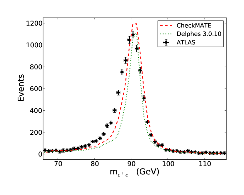
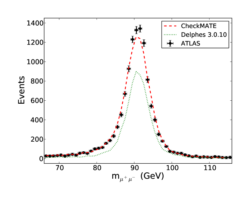
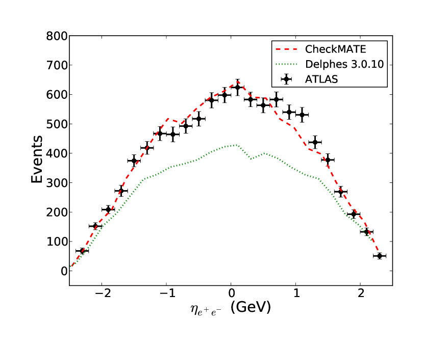
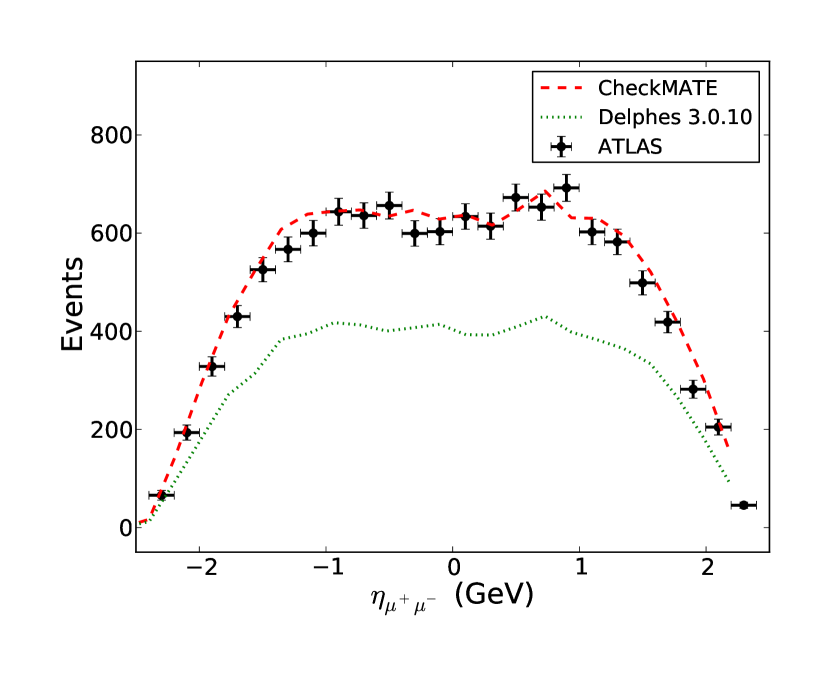
As stated in Section III.2, the default detector settings of Delphes have been significantly improved to match the latest ATLAS performance. In particular, all final state objects have been matched within the experimental uncertainties to the latest data available and the detailed results are given in Appendix C. These tunings have been validated by comparing with some ATLAS analyses of Standard Model processes. As an example we show the reconstruction of SM production141414Note that this analysis has been performed at and the efficiencies Checkmate used for the results shown in Figure 8 correspond to the detector performance during this phase. However, recently ATLAS improved their electron reconstruction and identification algorithms with better overall efficiency factors. Checkmate uses these updated results for its public version. versus ATLAS data for both electrons and muons in Figure 8. More detailed results are given in Appendix C.
Before any analysis is accepted into the the latest version of Checkmate it must be validated against the various data given in the published result. Whenever cutflows are given, these are checked at each step to make sure that all experimental cuts perform as expected, c.f. Appendix D. The majority of the cutflows we have evaluated with Checkmate have an acceptance that is within 10% of the published value for the signal regions. If this accuracy is not achieved, the analysis has been checked thoroughly to ensure no bugs remain and possible (or confirmed) reasons for the discrepancy are clearly stated, see Appendix D.

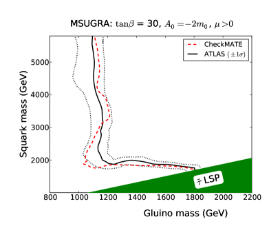
Many of the experimental analyses give exclusion curves for some popular (or simplified) models. Whenever possible these have been replicated by Checkmate (Appendix D) and in general the results lie within the 1 theoretical uncertainty predicted by the model. Again, in the rare occasions that the required accuracy has not been met, possible reasons for the discrepancy are given. An example parameter scan is shown in Figure 9 for the commonly studied SUSY model mSUGRA for the ATLAS jets and search (atlas_conf_2013_047) that shows agreement within the 1 theoretical uncertainty for almost the whole plane.
V.2 Computing Performance
As an example to show the relative computing time of Checkmate we consider an estimate from the ATLAS trilepton study (atlas_conf_2013_049). The generation of 1000 events in the HepMC format takes about 121 seconds of CPU time151515The CPU time performance has been tested on an Intel Core 2, Quad CPU with 2.4 GHz and 8 GB RAM. with Herwig++ 2.6.3. The Delphes 3.0.10 detector simulation with the relevant detector cards from Checkmate requires 11 seconds of CPU time. Once the detector simulation is finished, running the ATLAS trilepton analysis only takes about 1 second for all five signal regions. Thus the running time of the analysis is negligible compared to the event generation and detector simulation. This justifies our choice to closely match the cutflows of the experiments and thus add reliability and not to optimise the analyses for computing time performance.
VI Outlook
We would like to emphasise that while Checkmate is fully functional, it remains a work in progress. We will improve and extend the program over time.
At the moment, we have concentrated on searches for supersymmetry from ATLAS. However, the various supersymmetric analyses already cover multiple final state configurations and thus should be sensitive to many non–supersymmetric BSM physics scenarios containing invisible particles. Nevertheless, we want to implement as many of the new exotic searches from ATLAS and CMS as possible. We hope that the user will have access to an even larger selection of analyses in the near future.
Furthermore, we have decided to implement the results of the conferences notes rather than taking analyses from journal publications. Our decision is justified due to the fact that the majority of published results have not so far taken into account the 8 TeVdata and we are convinced that the implementation of studies with the best kinematical reach is the better alternative. As soon as the published results become available, we will update our studies.
Checkmate already provides a large number of validated analyses and many more only require final validation. Moreover, the structure of the program allows for easy implementation of additional analyses by any user. If an analysis has been programmed we would welcome the opportunity to include the study in the official Checkmate library. After the new analysis has been validated, it would then be made available to the whole user community.
As discussed, we have significantly improved the detector simulation performance of Delphes. However, we would like to implement even better detector tunings. In particular, when ATLAS and CMS publish updated detector performances, it is planned that we will revise the detector tunings to take advantage of the new information161616We would like to take this opportunity to plead with the collaborations to provide more detail in regards to detector performance. In particular, final state object maps for both identification and reconstruction should be provided in terms of and for all final state objects..
In addition to improving the analysis base of Checkmate, we further plan to present applications (case studies) to investigate models that the collaborations have not yet been able to complete and which we hope illustrate the power of Checkmate. When these studies are available we will publish programs that enable the user to repeat these studies and easily run new parameter scans themselves.
Further into the future we plan to significantly extend the functionality of Checkmate to aid usability. Firstly we plan to include a Monte-Carlo generator into the program so that users no longer have to generate event files themselves. Along with this innovation, will be a supersymmetry SLHA file reader requiring only a supersymmetric spectrum as input. For models other than supersymmetry we plan a close integration with FeynRules Alloul:2013bka and SARAH Staub:2013tta so that the user can begin their Checkmate investigations armed only with a Lagrangian.
VII Summary
We have introduced the program Checkmate, which is a tool to automatically check the compatibility of BSM models with LHC data. The program takes input in the form of Monte Carlo event files and cross-sections. These event files are given to a detector simulation and the result passed to implementations of LHC analyses. The outcome of the analyses is then compared to LHC results to see if the given model can be excluded.
The program has been designed for easy installation and operation. In addition, the structure allows the user to include new experimental analyses in a straightforward manner. However, it must be emphasised that the current analysis status in Checkmate is in no way considered complete. It is foreseen that many additional LHC new physics searches will be included in future upgrades.
The code can be obtained from the Checkmate webpage
http://checkmate.hepforge.org
as well as the installation instructions, more detailed technical informations and frequently asked questions.
Acknowledgements
We would especially like to thank Andreas Hoecker for many detailed discussions regarding ATLAS analyses. In addition, we would like to thank Philip Bechtle, Jamie Boyd, Geraldine Conti, Carolina Deluca, Klaus Desch, Monica D’Onofrio, Frank Filthaut, Eva Halkiadakis, Emma Kuwertz, Zachary Marshall, Antoine Marzin, Alaettin Serhan Mete, Marija Vranjes Milosavljevic, Maurizio Pierini, Tina Potter, George Redlinger, Steven Worm and Frank Wuerthwein for helpful discussions regarding different analyses. On the theoretical side, Tim Stefaniak provided useful advice from his work with ‘HiggsBounds/Signals’. The work has been supported by the BMBF grant 00160200. The work of M. Drees has been supported by the SFB TR33 ”The Dark Universe” funded by the Deutsche Forschungsgemeinschaft (DFG). The work of J. S. Kim has been partially supported by the MICINN, Spain, under contract FPA2010- 17747; Consolider-Ingenio CPAN CSD2007-00042 and by the ARC Centre of Excellence for Particle Physics at the Terascale. J. S. Kim also thanks the Spanish MINECO Centro de excelencia Severo Ochoa Program under grant SEV-2012-0249.
Appendix A Getting Started
This section guides the user through the installation of Checkmate and outlines how to check and potentially install updated versions of all the necessary prerequisites. The program has been tested and will run on both Linux and MacOS X171717The installation on MacOS X systems require the Xcode Command Line Tools. Details for the installation can be found on http://railsapps.github.io/xcode-command-line-tools.html and https://developer.apple.com/xcode/. Please note that wget is not pre-installed on MacOS X systems. However, it can be obtained from the MacPorts system https://www.macports.org or by downloading the respective files by hand.. An alternative online step–by–step tutorial can be found under http://checkmate.hepforge.org/tutorial/start.php.
Setting up Python
Checkmate requires Python 2.7.X with on your system. Most systems already come with a Python installation, which
you can easily check by typing python -V and hitting ‘enter’ in a terminal. If Python is installed, it should
start and immediately tell you the version number. If the installation is too old, too
new181818Checkmate does not work with Python 3. or if there is no Python at all, please install it
either manually from http://www.python.org/download/ or using the software management of your system.
Setting up Root
Checkmate uses Root for a variety of tasks, therefore it is necessary that
every user has a fully working Root installation available on their system.
Furthermore, Checkmate uses some Root packages which are not installed automatically and which may
need to be added. Due to the large size of the Root source code, we refrained from including it in
our package and only provide a step-by-step tutorial for how to install it from scratch or add
potentially missing obligatory packages to an existing installation. Running whereis root inside the terminal tells you if there already exists an installation on your system and determines how to continue with the installation:
- Case 1: There is no Root installed yet
-
You must download the source and install Root from scratch. Please do not use the Root pre-compiled binaries but follow these instructions, since we encountered internal linking problems with the binary version of Root. Start by downloading the latest version from http://root.cern.ch/drupal/content/downloading-root with:
wget ftp://root.cern.ch/root/root_xyz.source.tar.gzgzip -dc root_xyz.source.tar.gz | tar -xf -cd root
After downloading Root you can choose where you would like the installation located. If you don’t want to do a system-wide installation in
/usr/bin(e.g. because you do not have administrator rights), you have to use--prefixand--etcdirto declare the installation folder. Should you use a local Python installation (i.e. if the Python binary is not located in/usr/bin), you have to give the positions of both/includeand/libby adding--with-python-incdir=[path_to_python]/include/python2.7--with-python-libdir=[path_to_python]/libwith:./configure --enable-python --enable-roofit --enable-minuit2 {--prefix=[desired_root_path]} \ {--with-python-incdir=[path_to_python]/include/python2.7 --with-python-libdir=[path_to_python]/lib}make
Root is large, so go and have a (big) cup coffee in the meanwhile. After a successful completion, please hit:
make install
- Case 2: There is already a Root installation on the system.
-
If you already have Root on your system, let us first check if it includes all necessary packages. In the Root base directory, please run the following commands:
./bin/root-config --has-minuit2 ./bin/root-config --has-roofit ./bin/root-config --has-pythonIf all three commands return ‘yes’, your Root installation includes everything Checkmate needs and you can safely skip to the ‘Setting up Checkmate’ section. If not, you have to recompile the code and add the missing packages. Follow the instructions mentioned for ‘Case 1’, but make sure that
-
•
you download the same Root version the system has (you can use
./root-config --versionto find out), -
•
you install into the same root-directory by choosing
--prefixaccordingly. Alternatively, you can always download and install a second root version locally according to step 1. Make sure that you set up Checkmate with this local Root version explicitly.
In case you are using the standalone Root binaries, beware that we sometimes encountered problems during the compilation of Checkmate. Should you find the same problems, i.e. that all the aforementioned checks were positive but still there are Root linking errors occurring, please consider using a proper installation from source code as explained above.
-
•
Setting up Checkmate
Contrary to many other tools, Checkmate does not have a separate make install routine and
will set itself up in the directory you put it. You should therefore begin the following procedure
from within the folder you want Checkmate to be located.
Start by downloading the tarball either by hand or from within the terminal
wget http://www.hepforge.org/archive/checkmate/CheckMATE-Current.tar.gzExtract the tarball and have a look at the Checkmate folder:
tar -xvf CheckMATE-Current.tar.gz cd CheckMATE-X.Y.Z lsaclocal.m4 bin configure.ac depcomp m4 missing toolsAUTHORS ChangeLog COPYING INSTALL Makefile.am NEWS VERSIONautom4te.cache configure data install-sh Makefile.in READMEIn order to run Checkmate we have to compile the code, connect the Python scripts
to the Root libraries and create the binary. The configuration step will make sure
that you followed the aforementioned sections to properly setup Root and have a valid
Python interpreter. The easiest way to proceed is to run ./configure and follow the
instructions in case of an error. After successful configuration, type make191919Depending upon your
system the make command can generate various warning messages. These can be safely ignored unless the
final output is an error message (e.g. make: *** [all-recursive] Error 1) in which case the
installation will have failed. If you are unable to understand the cause of the problem, please check the
installation FAQ on the Checkmate website., which will
create a Checkmate binary in bin/.
./configure {--with-rootsys=[path_to_root]} {--with-python=[path_to_python]/bin/python} makeNote for experienced Root users: Checkmate should work even if you haven’t set up $ROOTSYS (and similar) environmental variables since it takes all information from the --with-rootsys parameter. However in case of any unexpected errors, run thisroot.(c)sh inside the Root binary directory and retry.
To test the installation, run the test parameter file in the bin directory.
cd bin ./CheckMATE testparam.datThe program will ask if the automatically chosen output directory is correct. After
answering ’y’ the program should run and finish with the statement that the
input is allowed. If it doesn’t, check whether your configuration and compilation
produced any errors or warnings. Otherwise, you finished setting up Checkmate and you
can continue with Section II to learn how you can run the code.
Appendix B Adding Analyses
Checkmate is not only meant to be simple to use and transparent. The philosophy of the program is that it is also supposed to be easy to extend with new ideas for analyses or users who need a particular analysis, which has not been implemented yet. In this section we give a brief introduction into the most important steps that are necessary to implement a new analysis.
B.1 Using the Analysis Manager
Checkmate comes with an Analysis Manager, i.e. a binary which asks the user for all the necessary details and takes care of the internal setup. In order to not confuse the normal user, this binary is not created automatically with the ordinary compilation of the code. However, it can easily be added by typing (after having already configured the code according to Appendix A)
make AnalysisManagerThis should create a second binary AnalysisManager within the bin/ folder. Running it will reveal three possible options:
-
•
Show a list of all currently implemented analyses,
-
•
add a new analysis/modify an existing analysis or
-
•
remove an analysis.
Choosing the second option will guide the user through a large list of
questions regarding the analysis. These gather information with respect to the
general properties of the analysis like name and luminosity, the setup of the detector
simulation (see Section III.2) and all the considered signal regions
with their respective experimental numbers for observation and background.
These settings are written in human–readable form in data/ANALYSIS_var.j and can be
changed afterwards, by re-running the ‘adding’ step with the
AnalysisManager202020Adding a new analysis will not only produce the described analysis variable file, but will also save the analysis information and the signal region numbers in separate auxiliary files, which are read by the respective Checkmate modules.
Changing the analysis variable file will not update these auxiliary files automatically.. Furthermore, the AnalysisManager creates ready–to–compile source and header files in tools/analysis/src and tools/analysis/include and adds them to the configuration files, such that they are compiled with the make routine.
B.2 Analysis Code
After the source files have been created, they have to be filled with the actual analysis code. For this, Checkmate provides a general C++ analysis framework using a globally defined base class212121The concept of the code structure is based on the Rivet analysis framework Buckley:2010ar .. This class provides particle containers for all the different types of final state objects, like leptons or jets, alongside with various methods that are commonly needed in many analyses, like phase space reduction and overlap removals.
To keep this manual at a reasonable volume, we will only show a minimal example to illustrate the basic structure of the code in Figure 10. For more details on the full list of implemented procedures, see the Checkmate webpage or the source code of the already implemented analyses.
#include "example.h" // The header file can stay untouched. void Example::initialize() { // This function is called once before the event loop. setAnalysisName("example"); // These set the header of all output files. setInformation("" "@#Example Analysis\n" ""); setLuminosity(10*units::INVFB); // Events are normalised to this integrated lumi. ignore("towers"); // These won’t read tower or track information from the ignore("tracks"); // Delphes output branches to save computing time. bookSignalRegions("jets;jets_plus_e;jets_plus_m"); // All signal- and cutflow regions to be used later have bookCutflowRegions("singlelep;twojets"); // to be defined here using a unique name. } void Example::analyze() { // This function is called once for each event. electronsMedium = filterPhaseSpace(electronsMedium, 20, -2.5, 2.5, true); // ’medium’ electrons, pT > 20 GeV, |eta| < 2.5, // excluding the region with 1.37 < |eta| < 1.52. std::vector<Electron*> isoElecs = filterIsolation(electronsMedium); // Whatever isolation cuts have been defined in the // analysis definition are applied here and the result // stored in a new container. muonsCombined = filterPhaseSpace(muonsCombined, 25, -2.0, 2.0); // ’combined’ muons, pT > 25 GeV, |eta| < 2.0. std::vector<Muon*> isoMuons = filterIsolation(muonsCombined); missingET->addMuons(isoMuons); // Muons are excluded from the missing energy calculation // in Delphes and have to be added manually. jets = filterPhaseSpace(jets, 50); // Jets, pT > 50 GeV. jets = overlapRemoval(jets, electronsMedium, 0.2); // Jets that overlap with an isolated electron with // dR < 0.2 are discarded. if (isoElecs.size() + isoMuons.size() == 1) // Veto event if it does not contain exactly one lepton. return; countCutflowEvent("singlelep"); // Count this event for the first cutflow step. if (jets.size() < 2) return; countCutflowEvent("twojets"); // Veto on events with less than 2 jets. double E_tot = 0; for(int j = 0; j < jets.size(); j++) // This loops over all jets and sums up their scalar ET. E_tot += jets[j]->PT; if (E_tot >= 150) { // Signal region 1: Sum(Scalar ET) > 150 GeV. countSignalEvent("jets"); if ((isoElecs.size() == 1)&& (fabs(isoElecs[0]->P4().DeltaPhi(missingET->P4())) < 0.3)) countSignalEvent("jets_plus_e"); // Signal Region 2: SR1 + an electron that lies close to // the missing momentum vector. else if ((isoMuons.size() == 1)&& (fabs(isoElecs[0]->P4().DeltaPhi(missingET->P4())) < 0.15)) countSignalEvent("jets_plus_m"); // Signal Region 3: SR1 + a muon that lies even closer to // the missing momentum vector. } } void Example::finalize() { // This function is called once after the event loop. } // However, usually there is nothing to do here.
The shown example consists of a fictitious analysis with three signal regions and a two-step cutflow. It considers isolated electrons with , passing the ‘medium’ identification requirement and not being in the overlap region . Furthermore it considers ‘combined’ muons and jets with different kinematical cuts. Jets that overlap with an isolated electron within are discarded. The event is also vetoed if it does not contain exactly one lepton and at least two jets. One signal region demands the total scalar sum of all isolated jet energies to be larger than 150 GeV. The second and third signal region requires an isolated electron or muon, respectively, that has a small angular separation from the missing momentum vector.
We finish this section with some important information regarding analyses in general:
-
•
Available particle containers are
electronsLoose, electronsMedium, electronsTight, muonsCombinedPlus,muonsCombined, jets, jets2, photons, tracksandtowers.jets2only contains data if a second jet type has been defined in the creation of the analysis.towersandtracksare not needed by many analyses and are hence ignored in the standard analysis initialisation, meaning that the Root branch is not read. -
•
These containers are of the standard C++ vector type, string pointers to the respective particle objects.
-
•
All vectors are sorted according to the objects’ , with e.g.
jets[0]having the highest transverse momentum. -
•
The final numbers for all signal–, control– and cutflow regions are automatically saved in the corresponding output file after the analysis run, listed in alphabetical order.
-
•
Calling the
P4()method returns the particle’s 4–vector in the lab frame, using Root’s TLorentzVector format which comes with a convenient list of applicable methods. -
•
The header file (
example.hin this case) can stay untouched in most cases. However, to save computing time it might be reasonable to not define local variables in theanalyze()method but instead define them as members of the analysis class within the header.
Appendix C ATLAS Detector Tunings
C.1 Jets and Photons
For both jets and photons, the standard Delphes parametrisations for reconstruction and identification have been used. Please see deFavereau:2013fsa for more details.
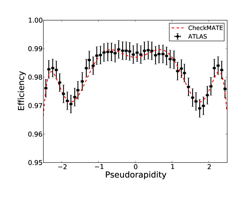
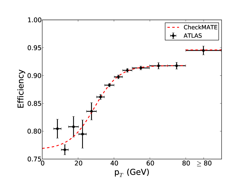
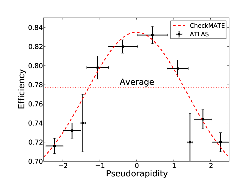
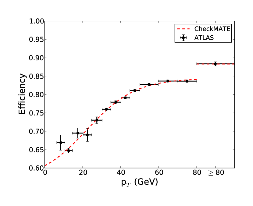
C.2 Electrons
The efficiencies for electron objects to be reconstructed as such are combined from the individually measured reconstruction and identification efficiency, for which the latter distinguishes between two kinds of electrons: ‘medium’ and ‘tight’222222The ’loose’ electron efficiency for identifying a truth-level electron is estimated by implementing a weak calorimeter isolation that mimics the ATLAS reconstruction. We require that within a cone size around the electron, at least 80% of energy deposition is due to the electron.. The reconstruction efficiency does not show any significant dependence on the candidate’s momentum but mostly on the pseudorapidity, as can be seen in Figure 11(a). Conversely, the identification efficiency for medium electrons mostly depends on the transverse energy of the electron, as shown in Figure 11(b), and insignificantly on its position. The total efficiency is given as the product of the two contributions and can be seen in a representative two-dimensional grid in Figure 12(a).
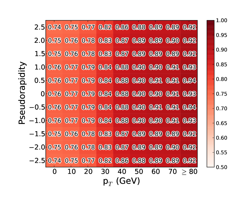
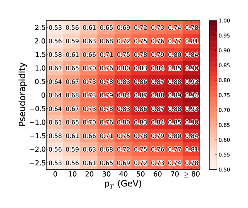
For ‘tight’ electrons, there exist measurements for both the pseudorapidity and the dependence of the identification efficiency individually, for which the corresponding other variable has been integrated over (see Figure 11(c) and Figure 11(d)). We normalise the pseudorapidity dependent function to an average value of unity and use as the overall identification efficiency the absolute efficiency with respect to , multiplied by the renormalised efficiency with respect to pseudorapidity. Combining this with the reconstruction efficiency described before leads to the total efficiency distribution shown in Figure 12(b).
The following functional behaviour for the efficiencies is used ( in GeV):
| (2) | ||||
| (6) | ||||
| (10) | ||||
| (11) |
C.3 Muons
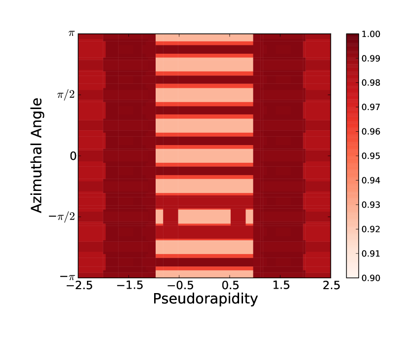
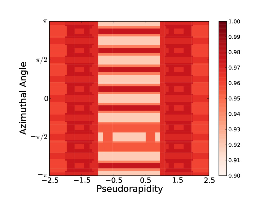
For muons, the main effect that has to be taken into account is the efficiency to reconstruct an object in the muon chambers and associate it to a track in the inner detector region. There exist two main quality criteria for this reconstruction, namely ‘Combined’ (requires both a track in the inner detector and muon chambers) and ‘Standalone’ (only requires a track in the muon chamber). The latter is usually used in combination with the first to maximise the muon efficiency and is hence called ‘Combined+Standalone’ (a standalone track is used when a combined track is not reconstructed).
The muon chambers in ATLAS consist of different components, which each have a different reconstruction probability, mainly caused by different types and quantities of material and the geometry inside the full detector. In Checkmate, we parametrised a detector-component map in the – plane and associate a particular efficiency to each detector type. The resulting two-dimensional grid232323We refrain from showing the functional description of the full map inside the main text, as the fine and irregular segmentation leads to a hard-to-read matrix. If further information is desired, the user should feel free to contact the authors. is shown in Figure 13.
C.4 B–Tagger
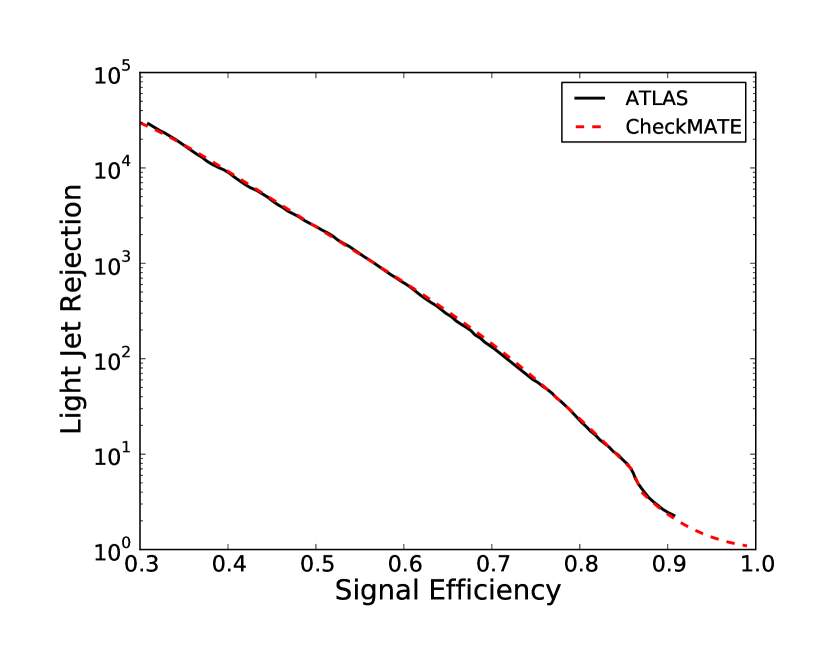
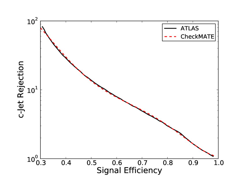
The quality of algorithms that try to filter jets containing b–quarks from others is determined by two main quantities: The signal efficiency describes the probability to assign a tag to a jet that actually contains a b–quark, whereas the background efficiency is a measure for the relative amount of jets that are tagged even though they don’t have any bottom quark content. Since the background efficiency is usually small, it is common to use the inverse value, called rejection, for illustrative purposes. Also, one usually distinguishes between rejections against jets with charm–content and other jets that only contain light quarks, as the first are harder to distinguish from the signal.
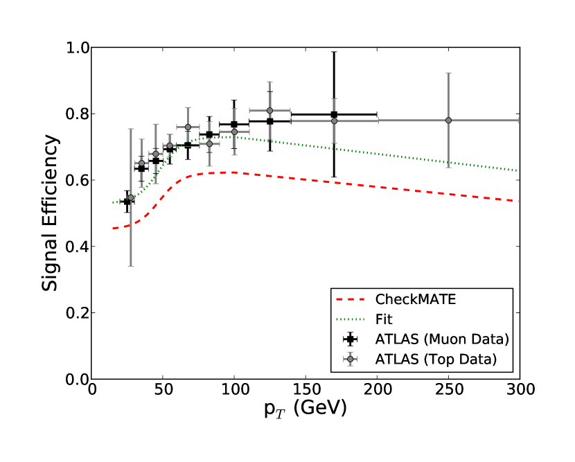
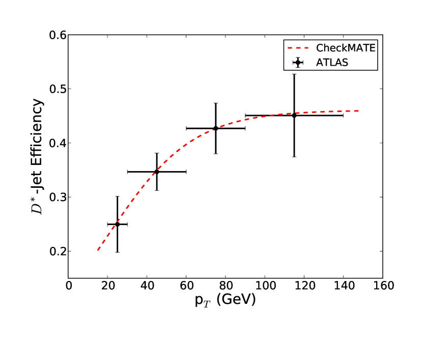
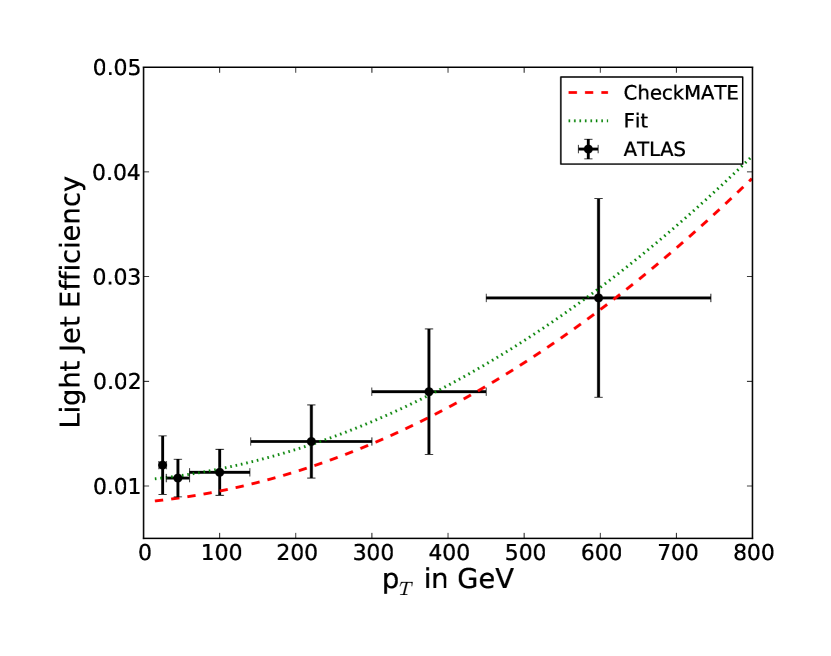
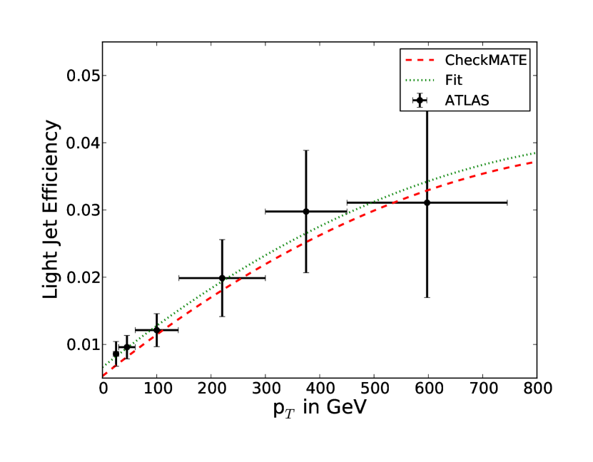
Since the rejection gets weaker with increasing signal efficiency, one has to find a balance between signal quantity and signal purity, which depends crucially on the details of the respective analysis. For this purpose, one uses the ROC (Receiver Operation Characteristic) curve that describes the relation between these two quantities. We show the ROC curves for light-jet rejection and c-jet rejection separately in Figure 14 and internally parametrise these as follows:
| (14) | ||||
| (15) |
Given a particular working point on the ROC curve, i.e. a specific chosen signal efficiency and the corresponding background rejections , the actual tagging probabilities depend on the transverse momentum of the considered object. These have been measured individually for signal–, light-quark– and meson242424The tagging probability for jets containing mesons is roughly 2 times better than for ‘normal’ c-quarks. Using the cutflows from various analyses we have tuned this parameter to 0.4 to be in agreement with the ATLAS results. jets and we show the results in Figure 15.
For the signal efficiency, we use two different data sets as they have different sensitivities at low and high energies (see Figure 15(a)). In order to agree with the cutflows of various analyses that require -tagging, a reduction in the overall normalisation by 15% has been applied. In addition, the significant decrease of the signal efficiency at large energies has been manually added in order to get better agreement with experimental results.
Furthermore, the light quark jet rejection has been measured for two different regions, which we adapt in our parametrisations. We also perform a reduction in the light-quark tagging rates (20%) in order to better agree with experimental cutflows.
Since the dependent distributions are given for a particular working point , we linearly rescale the functions to the given chosen signal efficiency , or the corresponding background efficiency given by the ROC curves ( in GeV):
| (19) | ||||
| (23) | ||||
| (24) |
C.5 Tau–Tagger
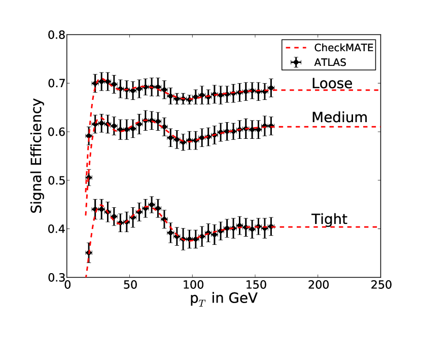
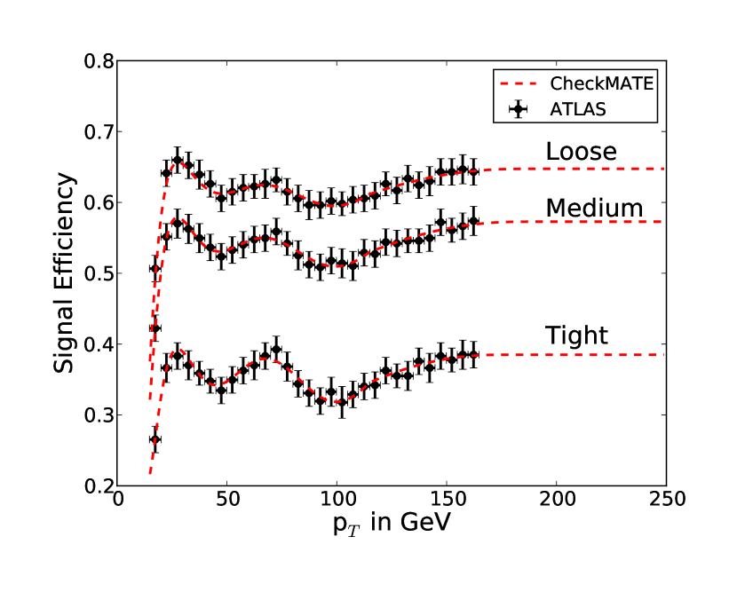
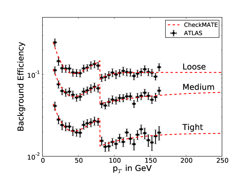
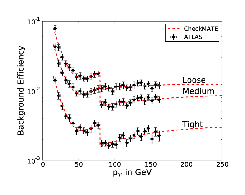
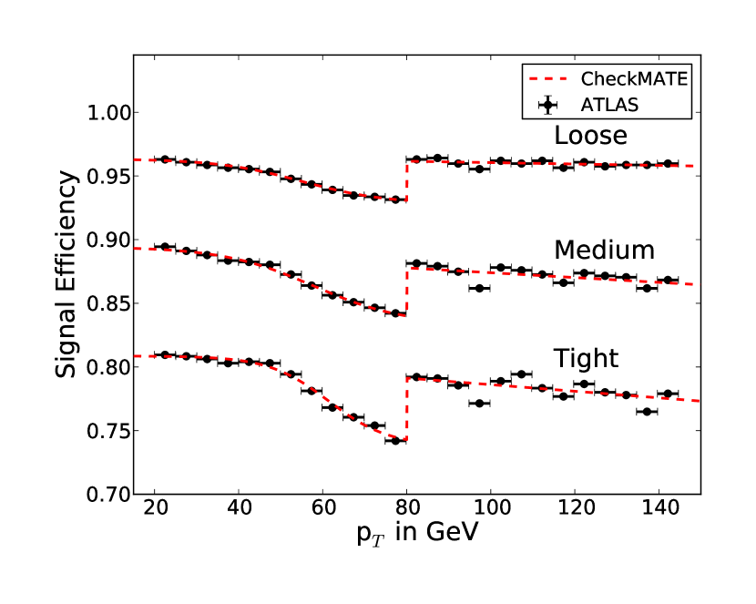
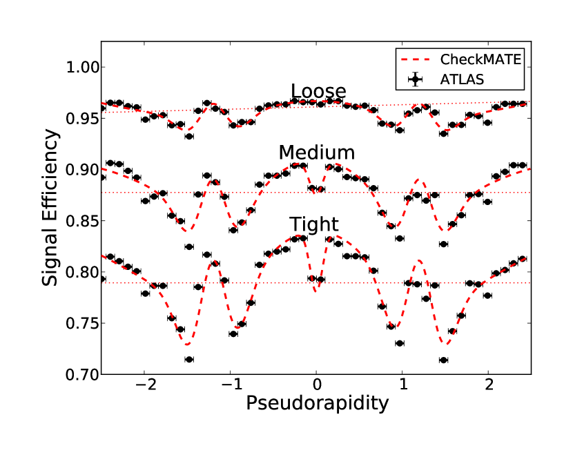
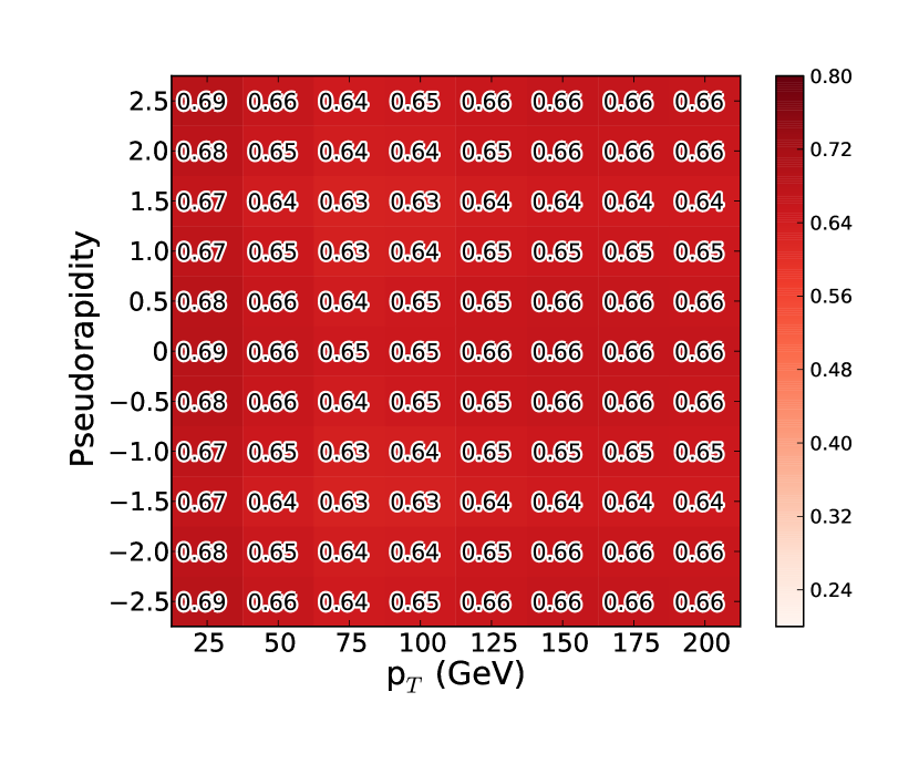
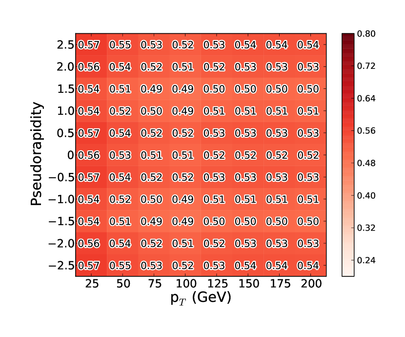
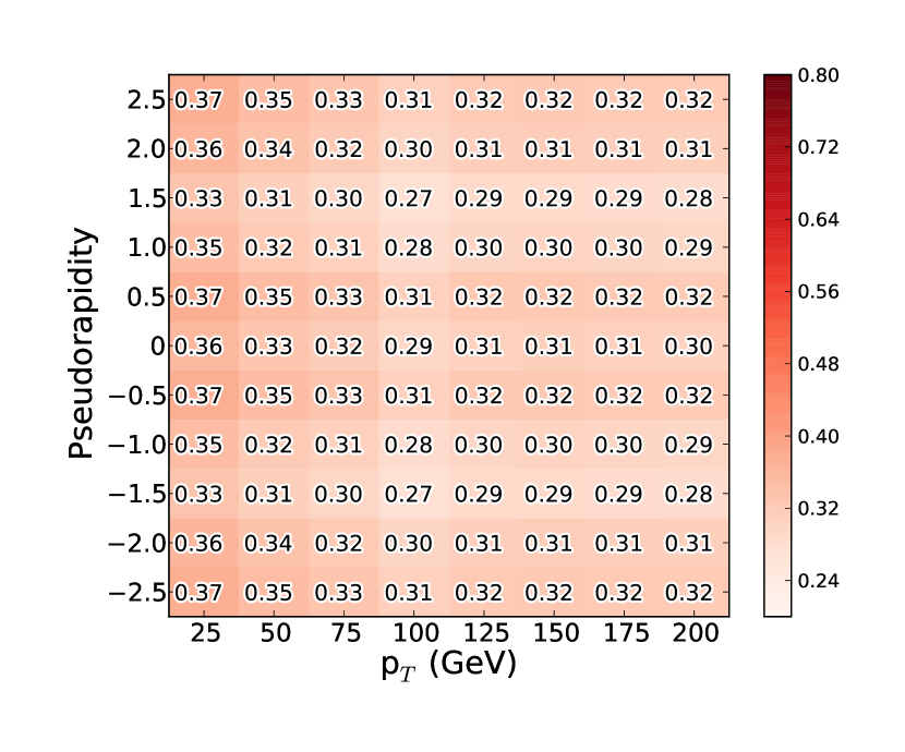
Analogously to the tagging of jets containing quarks, there exist algorithms to distinguish jets that originated from a hadronically decaying lepton from those that originated from quarks or gluons. Due to charge conservation, the lepton can only decay into an odd number of charged objects — mostly into 1 or 3 — called prongs. Since the structures of the resulting jets look rather different, identification algorithms usually differentiate between these two cases and hence there are individual efficiencies for each.
We show the efficiencies for signal and (light parton–)background with respect to the momentum of the jet candidate in Figure 16. Again, three common efficiency working points — ‘loose, ‘medium’ and ‘tight’ — are used in most analyses, and we show results for each of the three. The functional descriptions of the data points are shown in Equations 32 and 36, with the corresponding numerical values listed in Tables 3(a) and 3(b). For background and 3–prong jets, these are the final efficiency functions Checkmate uses. Note that these efficiencies do not depend on , but is always implied to fall within the angular coverage of the tracking detectors.
In addition to QCD jets, there is a second type of background which has to be taken into account: Electrons, which have been reconstructed as jets, can resemble 1–prong tau decays and need a separate tagging algorithm, which has been specifically tuned to reject these electron jets252525We only consider the impact on the signal efficiencies of this algorithm. In particular, we did not implement a specific mistagging efficiency for electrons. With the given Delphes code structure, any electron that fails the identification efficiency cut will be counted as a jet. Then, it will be tagged according to the corresponding background efficiency in Equation 36. Efficiencies with respect to this algorithm depend on both transverse momentum and pseudorapidity as shown in Figures 17(a) and 17(b). We follow the same approach as for the electron efficiencies, i.e. we take the absolute value from the momentum dependent efficiency distribution and multiply with the pseudorapidity distribution normalised to an average efficiency value of 1. The corresponding functions are shown in Equations 40 and 41 and Tables 3(c) and 3(d). We show a final combination of these with the 1–prong signal efficiency from before in Figures 18(a), 18(b) and 18(c) for each of the three working points ( in GeV):
| (28) | ||||
| (32) | ||||
| (36) | ||||
| (40) | ||||
| (41) |
| 1 prong, loose | 0.0223 | 1.16 | 0.427 | 0.846 | 0.670 | 100 | 0.0974 | 2.34 | 2.04 | ||
| 1 prong, medium | 0.0223 | 1.23 | 0.483 | 0.791 | 0.586 | 100 | 0.0997 | 2.23 | 1.91 | ||
| 1 prong, tight | 0.0292 | 1.17 | 0.377 | 0.799 | 0.388 | 100 | 0.101 | 2.16 | 1.79 | ||
| 3 prong, loose | 0.0192 | 0.143 | 0.106 | 1.08 | 0.594 | 99.6 | 0.0958 | 2.09 | 1.92 | ||
| 3 prong, medium | 0.0191 | 0.924 | 0.233 | 0.940 | 0.510 | 100 | 0.0950 | 2.18 | 1.86 | ||
| 3 prong, tight | 0.0212 | 0.671 | 0.104 | 1.096 | 0.324 | 100 | 0.0971 | 2.09 | 1.78 |
| 1 prong, loose | 0.717 | 0.106 | 64.3 | |||
| 1 prong, medium | 0.301 | 20.0 | ||||
| 1 prong, tight | 0.117 | 46.8 | ||||
| 3 prong, loose | 0.265 | 4.08 | ||||
| 3 prong, medium | 0.154 | 20.0 | ||||
| 3 prong, tight | 78.9 |
| loose | 0.94 | 0.875 | 0.294 | 0.886 | 0.286 | 1.16 | 10.9 | ||
| medium | 0.91 | 0.283 | 0.303 | 0.309 | 0.256 | 0.113 | 1.25 | ||
| tight | 0.84 | 0.472 | 0.304 | 0.503 | 0.258 | 0.102 | 1.42 |
| k | |||||||
|---|---|---|---|---|---|---|---|
| loose | 0.956 | 0.928 | 0.966 | ||||
| medium | 0.878 | 0.833 | 0.0922 | 57.8 | 0.893 | ||
| tight | 0.789 | 0.738 | 0.140 | 61.4 | 0.812 |
Appendix D Analysis Validation
D.1 atlas_conf_2012_104
1 lepton and . ATLAS-CONF-2012-104
Energy: 8 TeV
Luminosity: 5.8 fb-1
Validation notes:
-
•
Validation has been performed versus the published CMSSM (mSUGRA) parameter scan.
-
•
The exclusion in Checkmate is slightly weaker than the published ATLAS result, since ATLAS uses a different limit setting procedure. Checkmate only uses the signal region with the best expected sensitivity to set the limit. However, in this search ATLAS used a combined likelihood including all signal and control regions.
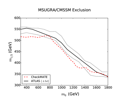
D.2 atlas_conf_2012_147
Monojet search, ATLAS-CONF-2012-147
Energy: 8 TeV
Luminosity: 10.5 fb-1
Validation notes:
-
•
Validation was performed against standard model and samples in signal region distributions of leading jet and .
-
•
The validation finishes with the hardest jet GeVdue to finite Monte-Carlo statistics.
-
•
No validation has yet been performed with parameter scans.
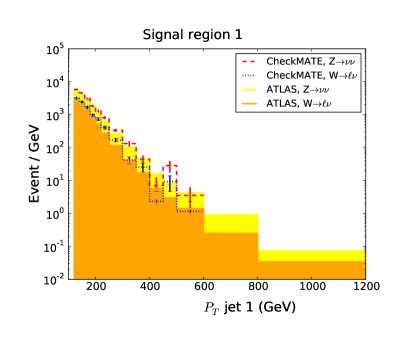
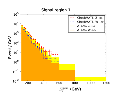
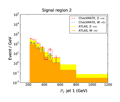
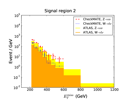
D.3 atlas_conf_2013_024
All-hadronic stop search, , ATLAS-CONF-2013-024
Energy: 8 TeV
Luminosity: 20.5 fb-1
Validation notes:
-
•
Validation has been performed versus all published cutflows and a simplified model consisting of pure stop production followed by the decay .
| Process | direct | |||
|---|---|---|---|---|
| Point | GeV | |||
| GeV | ||||
| Top Polarization | Right-handed | Left-handed | ||
| Source | ATLAS | Checkmate | ATLAS | Checkmate |
| No selection | 507.3 | 507.3 | 507.3 | 507.3 |
| Trigger | 468.0 | 469.7 | 467.8 | 468.8 |
| Primary vertex * | 467.8 | - | 467.4 | - |
| Event Cleaning * | 459.0 | - | 459.6 | - |
| Muon veto | 381.2 | 380.1 | 382.5 | 380.4 |
| Electron veto | 284.4 | 297.6 | 292.3 | 302.2 |
| 130 GeV | 263.1 | 275.4 | 270.1 | 277.7 |
| Jet multiplicity and | 97.7 | 95.0 | 92.2 | 87.3 |
| 30 GeV | 96.3 | 93.5 | 90.5 | 85.9 |
| 90.3 | 89.4 | 84.3 | 82.2 | |
| 77.1 | 76.0 | 72.0 | 69.2 | |
| Tau veto | 67.4 | 66.6 | 61.9 | 59.3 |
| -tagged jets | 29.5 | 28.6 | 31.5 | 27.9 |
| 175 GeV | 20.2 | 20.2 | 23.6 | 21.3 |
| 80 GeV 175 GeV | 17.8 | 18.4 | 20.4 | 19.3 |
| 80 GeV 175 GeV | 10.9 | 10.8 | 11.9 | 10.9 |
| 150 GeV | 10.8 | 10.7 | 11.8 | 11.8 |
| 200 GeV(SR1) | 10.3 | 10.2 | 11.2 | 10.5 |
| 250 GeV | 9.2 | 9.3 | 10.0 | 9.3 |
| 300 GeV(SR2) | 7.8 | 8.1 | 8.3 | 8.1 |
| 350 GeV(SR3) | 6.1 | 6.2 | 6.6 | 6.5 |
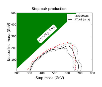
D.4 atlas_conf_2013_035
Trilepton, 0 jets + , ATLAS-CONF-2013-035
Energy: 8 TeV
Luminosity: 20.7 fb-1
Validation notes:
-
•
Validation has been performed versus all published cutflows.
| Process | production; decay via / or slepton | |||||
|---|---|---|---|---|---|---|
| Point | Simplified | Simplified WZ | Simplified | |||
| GeV | GeV | GeV | ||||
| GeV | GeV | GeV | ||||
| SRnoZa | SRnoZb | SRnoZc | ||||
| Source | ATLAS | Checkmate | ATLAS | Checkmate | ATLAS | Checkmate |
| Generated events | 25000 | 40000 | 20000 | 40000 | 40000 | 40000 |
| Lepton multiplicity | 537.1 | 688.1 | 227.3 | 278.8 | 28.5 | 28.1 |
| SFOS requirement | 536.3 | 615 | 226.5 | 272.5 | 28.1 | 27.9 |
| b veto | 491.0 | 557.4 | 211.0 | 251 | 24.9 | 24.8 |
| Z veto/request | 476.3 | 537 | 196.6 | 235 | 24.1 | 24 |
| 161.2 | 181.3 | 53.8 | 56.2 | 22.1 | 22 | |
| 141.2 | 154.2 | 27.1 | 26.8 | - | - | |
| - | - | - | - | 19.2 | 19 | |
| - | - | - | - | |||
| SRnoZc veto | - | - | ||||
| Process | production; decay via / or slepton | |||||
|---|---|---|---|---|---|---|
| Point | Simplified WZ | Simplified WZ | Simplified WZ | |||
| GeV | GeV | GeV | ||||
| GeV | GeV | GeV | ||||
| SRZa | SRZb | SRZc | ||||
| Source | ATLAS | Checkmate | ATLAS | Checkmate | ATLAS | Checkmate |
| Generated events | 15000 | 40000 | 20000 | 40000 | 20000 | 40000 |
| Lepton multiplicity | 1071.4 | 1118.9 | 259.8 | 276.9 | 40.0 | 44.2 |
| SFOS requirement | 1067.5 | 1109.5 | 258.0 | 273.9 | 39.7 | 43.7 |
| b veto | 989.4 | 1039 | 240.0 | 254.6 | 36.4 | 39.8 |
| Z veto/request | 912.7 | 866.5 | 227.2 | 227.1 | 34.4 | 34.9 |
| 170.7 | 135.9 | 67.7 | 66.5 | 17.7 | 17.3 | |
| - | - | - | - | - | - | |
| - | - | - | - | - | - | |
| SRnoZc veto | - | - | - | - | - | - |
D.5 atlas_conf_2013_047
0 lepton + 2-6 jets + , ATLAS-CONF-2013-047
Energy: 8 TeV
Luminosity: 20.3 fb-1
Validation notes:
-
•
Validation has been performed versus all published cutflows.
-
•
Additional validation has been performed with the parameter scan of the CMSSM (mSUGRA) model shown in Figure 9.
| Process | direct | |||||
|---|---|---|---|---|---|---|
| Point | GeV | GeV | GeV | |||
| GeV | GeV | GeV | ||||
| Signal Region | A-medium | A-medium | C-medium | |||
| Source | ATLAS | Checkmate | ATLAS | Checkmate | ATLAS | Checkmate |
| Generated events | 20000 | 50000 | 5000 | 50000 | 5000 | 50000 |
| Jet Cleaning * | 99.7 | - | 99.6 | - | 99.6 | - |
| 0-lepton * | 89.9 | - | 98.5 | - | 98.2 | - |
| 160 GeV* | 15 | - | 89.9 | - | 80.7 | - |
| 130 GeV | 12.9 | 12.9 | 89.7 | 89.5 | 80.0 | 79.3 |
| 130 GeV | 9.0 | 8.4 | 87.4 | 87.1 | 75.6 | 75.3 |
| 0-60 GeV | 9.0 | 8.4 | 87.4 | 87.1 | 35.3 | 35.6 |
| 0-60 GeV | 9.0 | 8.4 | 87.4 | 87.1 | 11.5 | 11.3 |
| 7.0 | 6.8 | 79.2 | 79.0 | 10.1 | 9.9 | |
| 7.0 | 6.8 | 79.2 | 79.0 | 9.3 | 9.2 | |
| 2.6 | 1.8 | 49.9 | 48.0 | 9.3 | 9.2 | |
| 2.6 | 1.8 | 49.9 | 48.0 | 7.2 | 6.8 | |
| TeV | ||||||
| Process | direct | direct | ||||
|---|---|---|---|---|---|---|
| Point | GeV | GeV | GeV | |||
| GeV | GeV | GeV | ||||
| Signal Region | B-medium | B-tight | D | |||
| Source | ATLAS | Checkmate | ATLAS | Checkmate | ATLAS | Checkmate |
| Generated events | 5000 | 50000 | 5000 | 50000 | 5000 | 50000 |
| Jet Cleaning * | 99.7 | - | 99.6 | - | 99.8 | - |
| 0-lepton * | 98.0 | - | 98.8 | - | 98.5 | - |
| 160 GeV* | 93.3 | - | 95.9 | - | 88.9 | - |
| 130 GeV | 93.3 | 93.9 | 95.8 | 96.0 | 88.8 | 88.1 |
| 130 GeV | 92.4 | 92.7 | 95.2 | 95.1 | 88.8 | 88.1 |
| 0-60 GeV | 68.5 | 67.0 | 75.7 | 73.5 | 87.1 | 86.8 |
| 0-60 GeV | 68.5 | 67.0 | 75.7 | 73.5 | 74.1 | 74.4 |
| 0-60 GeV | 68.5 | 67.0 | 75.7 | 73.5 | 40.9 | 36.0 |
| 60.4 | 58.7 | 66.2 | 64.2 | 34.2 | 30.1 | |
| 60.4 | 58.7 | 66.2 | 64.2 | 28.6 | 25.9 | |
| 44.8 | 41.8 | 31.8 | 28.1 | 22.1 | 18.9 | |
| TeV | ||||||
| Process | one-step ( decay via ) | |||
|---|---|---|---|---|
| Point | GeV | GeV | ||
| GeV | GeV | |||
| GeV | GeV | |||
| Signal Region | D | E-tight | ||
| Source | ATLAS | Checkmate | ATLAS | Checkmate |
| Generated events | 20000 | 50000 | 20000 | 50000 |
| Jet Cleaning * | 99.8 | - | 99.8 | - |
| 0-lepton * | 63.7 | - | 63.5 | - |
| 160 GeV* | 50.0 | - | 55.6 | - |
| 130 GeV | 49.3 | 47.7 | 55.6 | 54.4 |
| 130 GeV | 49.2 | 47.6 | 55.6 | 54.4 |
| 0-60 GeV | 48.6 | 47.1 | 55.4 | 54.2 |
| 0-60 GeV | 44.5 | 43.8 | 53.4 | 52.8 |
| 0-60 GeV | 34.4 | 34.8 | 46.3 | 46.6 |
| 0-60 GeV | 34.4 | 34.8 | 31.7 | 33.0 |
| 29.2 | 29.5 | 26.5 | 27.5 | |
| 24.6 | 24.7 | 21.3 | 22.4 | |
| 21.6 | 21.2 | 12.0 | 11.2 | |
| TeV | ||||
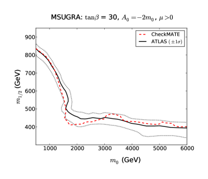

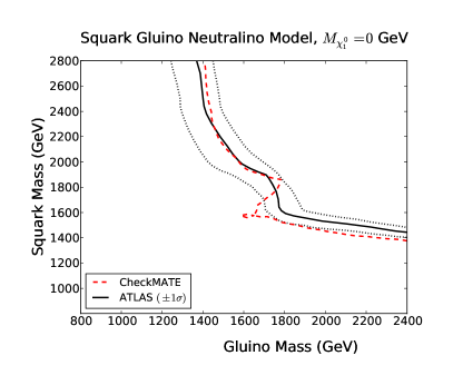
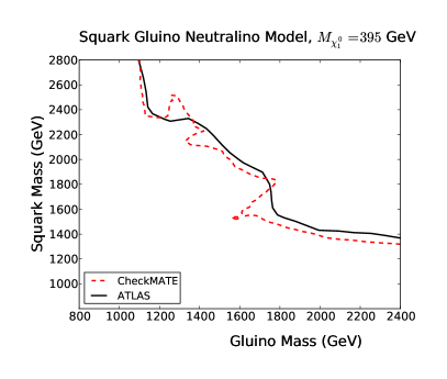
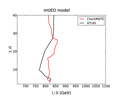
D.6 atlas_conf_2013_049
2 opposite-sign leptons, 0 jets + , ATLAS-CONF-2013-049
Energy: 8 TeV
Luminosity: 20.3 fb-1
Validation notes:
-
•
Validation has been performed versus all published cutflows.
-
•
Jet veto conditions have been tightened by 25% compared to the corresponding stated ATLAS values. This was done to match cutflow values and account for pile-up effects that Checkmate cannot simulate.
-
•
WARNING: For simplified models with chargino production and weak boson mediated decay, Checkmate systematically underestimates signal region cutflows. Despite much effort, no reason for this discrepancy has been found. The corresponding setting is conservative since it will not lead to spurious model exclusion.
-
•
No validation has yet been performed with parameter scans.
| Process | production | |||||||
|---|---|---|---|---|---|---|---|---|
| Point | GeV | GeV | ||||||
| GeV | GeV | |||||||
| Source | ATLAS | Checkmate | ATLAS | Checkmate | ATLAS | Checkmate | ATLAS | Checkmate |
| Generated events | 5000 | 50000 | 5000 | 50000 | 5000 | 50000 | 5000 | 50000 |
| Trigger | 150 | 153 | 159 | 153 | 55 | 55 | 50 | 50 |
| 139 | 143 | 148 | 142 | 54 | 52 | 49 | 48 | |
| Jet veto | 58 | 62 | 62 | 61 | 20 | 22 | 20 | 21 |
| GeV | 45 | 47 | 50 | 47 | 17 | 19 | 17 | 18 |
| SR- | ||||||||
| SR- | ||||||||
| Process | production, slepton decay | |||||
|---|---|---|---|---|---|---|
| Point | GeV | |||||
| GeV | ||||||
| GeV | ||||||
| Source | ATLAS | Checkmate | ATLAS | Checkmate | ATLAS | Checkmate |
| Generated events | 40000 | 50000 | 40000 | 50000 | 40000 | 50000 |
| Trigger | 52 | 50 | 48 | 49 | 79 | 74 |
| 48 | 47 | 45 | 46 | 74 | 69 | |
| Jet veto | 20 | 20 | 19 | 20 | 30 | 29 |
| GeV | 17 | 17 | 17 | 17 | 25 | 25 |
| SR- | ||||||
| SR- | ||||||
| Process | production, slepton decay | |||||
|---|---|---|---|---|---|---|
| Point | GeV | |||||
| GeV | ||||||
| GeV | ||||||
| Source | ATLAS | Checkmate | ATLAS | Checkmate | ATLAS | Checkmate |
| Generated events | 40000 | 50000 | 40000 | 50000 | 40000 | 50000 |
| Trigger | 20 | 21 | 20 | 20 | 31 | 30 |
| 19 | 20 | 19 | 19 | 29 | 28 | |
| Jet veto | 7 | 8 | 7 | 8 | 11 | 11 |
| GeV | 6 | 7 | 6 | 7 | 9 | 10 |
| SR- | ||||||
| SR- | ||||||
| Process | production, decay | |||||
|---|---|---|---|---|---|---|
| Point | GeV | GeV | GeV | |||
| GeV | GeV | GeV | ||||
| Source | ATLAS | Checkmate | ATLAS | Checkmate | ATLAS | Checkmate |
| Generated events | 20000 | 50000 | 20000 | 50000 | 20000 | 50000 |
| No Cuts | 11003 | - | 3393 | - | 749 | - |
| All Cleaning * | 10691 | 10673 | 3299 | 3289 | 732 | 727 |
| Two signal leptons | 3178 | 2610 | 1060 | 898 | 261 | 218 |
| Trigger | 2559 | 1977 | 872 | 684 | 214 | 167 |
| 861 | 803 | 296 | 288 | 71 | 69 | |
| Jet veto | 443 | 437 | 139 | 152 | 31 | 34 |
| GeV | 310 | 302 | 103 | 111 | 25 | 27 |
| SR-WWa | - | - | - | - | ||
| SR-WWb | - | - | - | - | ||
| SR-WWc | - | - | - | - | ||
D.7 atlas_conf_2013_061
Search for strong production with at least three -jets + , ATLAS-CONF-2013-061
Energy: 8 TeV
Luminosity: 20.1 fb-1
Validation notes:
-
•
Validation has been performed versus all published cutflows.
-
•
B-tagging efficiency was reduced by 3% compared with the nominal value in the experimental paper to better agree with cutflow data.
-
•
No validation has yet been performed with parameter scans.
| Process | ||||||
|---|---|---|---|---|---|---|
| Point | GeV, GeV | |||||
| Channel | 0 Lepton, 4 Jets | |||||
| Source | ATLAS | Checkmate | ||||
| No selection | 100 % | - % | ||||
| Jet and Event cleaning * | 98.2 % | - % | ||||
| Cosmic muon rejection * | 98.2 % | - % | ||||
| 4 jets ( GeV) | 95.4 % | 94.6 % | ||||
| 1st jet GeV | 95.4 % | 94.6 % | ||||
| 150 GeV | 88.7 % | 88.0 % | ||||
| Electron veto | 88.7 % | 86.1 % | ||||
| Muon veto | 88.2 % | 85.7 % | ||||
| 58.5 % | 59.9 % | |||||
| 46.2 % | 48.7 % | |||||
| Signal region cuts | SR-0l-4j-A | SR-0l-4j-B | SR-0l-4j-C | |||
| Source | ATLAS | Checkmate | ATLAS | Checkmate | ATLAS | Checkmate |
| , | 46.2 % | 48.7 % | 42.8 % | 45.3 % | 42.8 % | 45.3 % |
| , | 20.5 % | 20.0 % | 17.9 % | 17.5 % | 17.9 % | 17.4 % |
| 200, 350, 250 | 20.5 % | 19.9 % | 16.2 % | 15.7 % | 17.4 % | 17.1 % |
| 1000, 1100, 1300 | 20.3 % | 19.7 % | % | % | % | % |
| 16, 0, 0 | % | % | - | - | - | - |
| Process | ||||||
|---|---|---|---|---|---|---|
| Point | GeV, GeV | |||||
| Channel | 0 Lepton, 7 Jets | |||||
| Source | ATLAS | Checkmate | ||||
| No selection | 100 % | - % | ||||
| Jet and Event cleaning * | 98.4 % | - % | ||||
| Cosmic muon rejection * | 97.2 % | - % | ||||
| 4 jets ( GeV) | 96.9 % | 97.6 % | ||||
| 1st jet GeV | 96.9 % | 97.5 % | ||||
| 150 GeV | 88.3 % | 87.7 % | ||||
| Electron veto | 59.7 % | 60.2 % | ||||
| Muon veto | 41.8 % | 40.7 % | ||||
| 30.0 % | 29.6 % | |||||
| 25.9 % | 25.4 % | |||||
| 7 jets ( GeV) | 24.6 % | 24.1 % | ||||
| 3 -jets ( GeV) | 11.5 % | 11.4 % | ||||
| Signal region cuts | SR-0l-7j-A | SR-0l-7j-B | SR-0l-7j-C | |||
| Source | ATLAS | Checkmate | ATLAS | Checkmate | ATLAS | Checkmate |
| 200, 350, 250 | 11.3 % | 11.3 % | 9.2 % | 8.9 % | 10.8 % | 10.8 % |
| 1000, 1000, 1500 | % | % | % | % | % | % |
| Process | ||||||
|---|---|---|---|---|---|---|
| Point | GeV, GeV | |||||
| Channel | 1 Lepton | |||||
| Source | ATLAS | Checkmate | ||||
| No selection | 100 % | - % | ||||
| Jet and Event cleaning * | 98.4 % | - % | ||||
| Cosmic muon rejection * | 97.2 % | - % | ||||
| 4 jets ( GeV) | 96.9 % | 97.6 % | ||||
| 1st jet GeV | 96.8 % | 97.5 % | ||||
| 150 GeV | 88.3 % | 87.5 % | ||||
| 1 signal lepton | 37.0 % | 40.6 % | ||||
| 6 jets GeV) | 33.8 % | 36.7 % | ||||
| 3 -jets ( GeV) | 14.3 % | 16.1 % | ||||
| Signal region cuts | SR-1l-6j-A | SR-1l-6j-B | SR-1l-6j-C | |||
| Source | ATLAS | Checkmate | ATLAS | Checkmate | ATLAS | Checkmate |
| 140, 140, 160 GeV | 11.3 % | 12.0 % | 11.3 % | 12.0 % | 10.7 % | 11.3 % |
| 175, 225, 275 GeV | 10.9 % | 11.6 % | 10.0 % | 10.7 % | 8.8 % | 9.3 % |
| 5 GeV1/2 | 10.8 % | 11.3 % | 10.0 % | 10.6 % | 8.8 % | 9.3 % |
| 700, 800, 900 GeV | % | % | % | % | % | % |
D.8 atlas_conf_2013_089
Strongly produced SUSY with two leptons (razor), ATLAS-CONF-2013-089
Energy: 8 TeV
Luminosity: 20.3 fb-1
Validation notes:
-
•
Validation has been performed versus all published cutflows.
-
•
WARNING: Discrepancies exist in the final signal regions between ATLAS and Checkmate. However, we do not believe this shows a systematic failing of Checkmate. First of all, the statistics from ATLAS are very small and it is therefore hard to draw a definitive conclusion. Moreover, after the trigger has been performed, no cut has an obvious flavour dependence. Consequently it is expected (and confirmed by ATLAS) that the channels should contain the largest number of events.
-
•
We see a difference in the exclusion for low squark masses and a heavier LSP. We believe this is due to different settings in the Monte Carlo parton shower (Pythia 6) that gives a harder initial state radiation distribution.
| Process | production, , | |||||
|---|---|---|---|---|---|---|
| Point | GeV, GeV, GeV | |||||
| Source | ATLAS | Checkmate | ||||
| No Cuts | 59999 | 59999 | ||||
| 2 baseline leptons | 2073 | 1880 | ||||
| Passes trigger | 1670 | 1426 | ||||
| GeV | 1639 | 1408 | ||||
| Lepton flavour | ||||||
| Source | ATLAS | Checkmate | ATLAS | Checkmate | ATLAS | Checkmate |
| Lepton separation | 576 | 420 | 397 | 397 | 666 | 590 |
| Signal leptons | 443 | 377 | 373 | 397 | 549 | 561 |
| Trigger + dilepton | 429 | 377 | 358 | 397 | 517 | 561 |
| jets, -veto | 341 | 320 | 297 | 350 | 424 | 480 |
| -veto | 319 | 293 | 276 | 321 | 424 | 480 |
| 139 | 155 | 137 | 162 | 195 | 252 | |
| GeV | ||||||
| jets, -veto | 53 | 44 | 40 | 34 | 54 | 56 |
| -veto | 51 | 41 | 36 | 31 | 54 | 56 |
| 16 | 14 | 19 | 10 | 12 | 21 | |
| GeV | ||||||
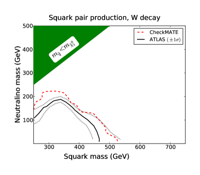
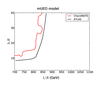
D.9 cms_1303_2985
Hadronic and jet multiplicity, Chatrchyan:2013lya
Energy: 8 TeV
Luminosity: 11.7 fb-1
Validation notes:
-
•
No cut flow is provided by CMS, validation is performed with signal region distributions and parameter scans.
-
•
The SM background distributions has been taken from the CMS note.
-
•
The ATLAS -tagging has been used.
-
•
Jumps in limit in Checkmate parameter scans are due to the single signal region limit setting procedure used (see Section I.2).
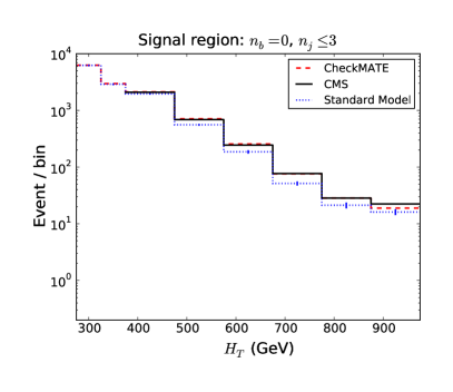
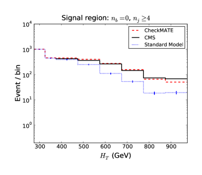
.
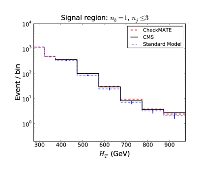
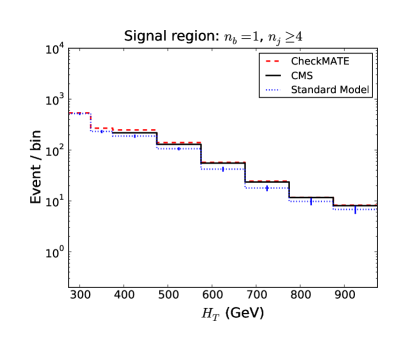
.
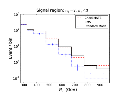
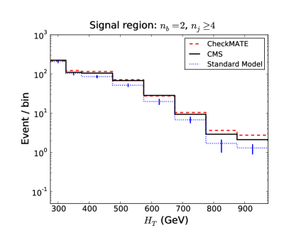
.
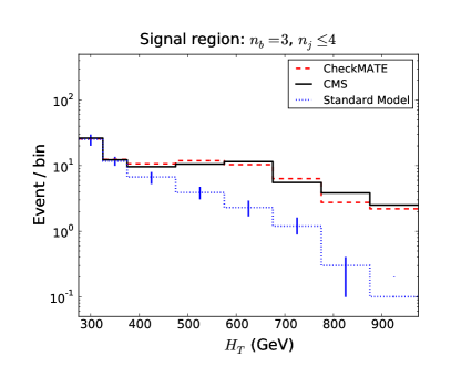
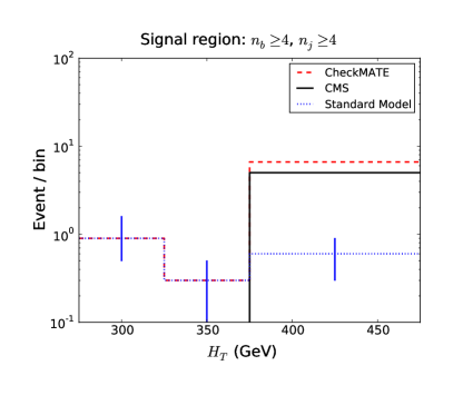
.
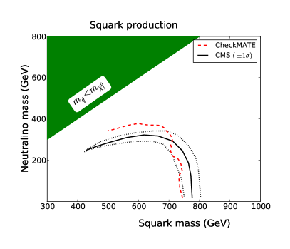
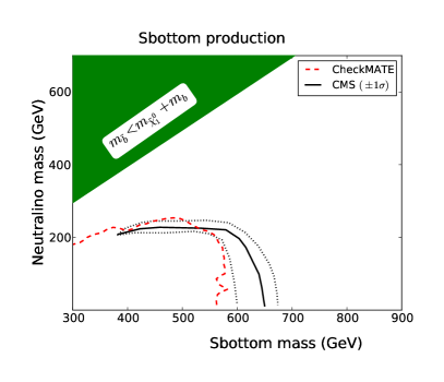
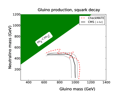
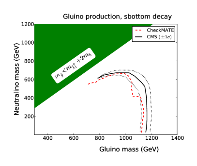
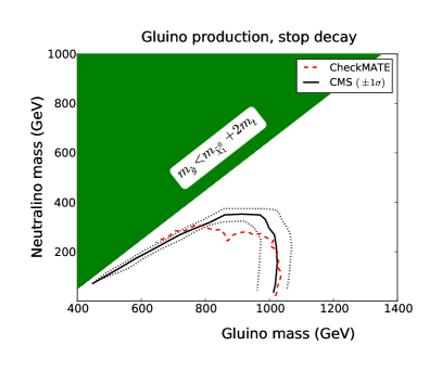
References
- (1) J. de Favereau, C. Delaere, P. Demin, A. Giammanco, V. Lemaître, et al., “DELPHES 3, A modular framework for fast simulation of a generic collider experiment,” 2013.
- (2) M. Cacciari, G. P. Salam, and G. Soyez, “FastJet User Manual,” Eur.Phys.J., vol. C72, p. 1896, 2012.
- (3) M. Cacciari and G. P. Salam, “Dispelling the myth for the jet-finder,” Phys.Lett., vol. B641, pp. 57–61, 2006.
- (4) M. Cacciari, G. P. Salam, and G. Soyez, “The Anti-k(t) jet clustering algorithm,” JHEP, vol. 0804, p. 063, 2008.
- (5) A. L. Read, “Presentation of search results: the cl’s technique,” Journal of Physics G: Nuclear and Particle Physics, vol. 28, no. 10, p. 2693, 2002.
- (6) C. Lester and D. Summers, “Measuring masses of semiinvisibly decaying particles pair produced at hadron colliders,” Phys.Lett., vol. B463, pp. 99–103, 1999.
- (7) A. Barr, C. Lester, and P. Stephens, “m(T2): The Truth behind the glamour,” J.Phys., vol. G29, pp. 2343–2363, 2003.
- (8) H.-C. Cheng and Z. Han, “Minimal Kinematic Constraints and m(T2),” JHEP, vol. 0812, p. 063, 2008.
- (9) H. E. Haber and G. L. Kane, “The Search for Supersymmetry: Probing Physics Beyond the Standard Model,” Phys.Rept., vol. 117, pp. 75–263, 1985.
- (10) H. P. Nilles, “Supersymmetry, Supergravity and Particle Physics,” Phys.Rept., vol. 110, pp. 1–162, 1984.
- (11) S. Weinberg, “Implications of Dynamical Symmetry Breaking,” Phys.Rev., vol. D13, pp. 974–996, 1976.
- (12) L. Susskind, “Dynamics of Spontaneous Symmetry Breaking in the Weinberg-Salam Theory,” Phys.Rev., vol. D20, pp. 2619–2625, 1979.
- (13) N. Arkani-Hamed, S. Dimopoulos, and G. Dvali, “The Hierarchy problem and new dimensions at a millimeter,” Phys.Lett., vol. B429, pp. 263–272, 1998.
- (14) L. Randall and R. Sundrum, “A Large mass hierarchy from a small extra dimension,” Phys.Rev.Lett., vol. 83, pp. 3370–3373, 1999.
- (15) D. Alves et al., “Simplified Models for LHC New Physics Searches,” J.Phys., vol. G39, p. 105005, 2012.
- (16) G. Bertone, D. Hooper, and J. Silk, “Particle dark matter: Evidence, candidates and constraints,” Phys.Rept., vol. 405, pp. 279–390, 2005.
- (17) M. Dobbs and J. B. Hansen, “The HepMC C++ Monte Carlo event record for High Energy Physics,” Comput.Phys.Commun., vol. 134, pp. 41–46, 2001.
- (18) I. Knowles, T. Sjostrand, A. Blondel, A. Boehrer, C. Buchanan, et al., “QCD event generators,” 1995.
- (19) T. Sjostrand, S. Mrenna, and P. Z. Skands, “PYTHIA 6.4 Physics and Manual,” JHEP, vol. 0605, p. 026, 2006.
- (20) T. Sjostrand, S. Mrenna, and P. Z. Skands, “A Brief Introduction to PYTHIA 8.1,” Comput.Phys.Commun., vol. 178, pp. 852–867, 2008.
- (21) M. Bahr, S. Gieseke, M. Gigg, D. Grellscheid, K. Hamilton, et al., “Herwig++ Physics and Manual,” Eur.Phys.J., vol. C58, pp. 639–707, 2008.
- (22) A. Belyaev, N. D. Christensen, and A. Pukhov, “CalcHEP 3.4 for collider physics within and beyond the Standard Model,” Comput.Phys.Commun., vol. 184, pp. 1729–1769, 2013.
- (23) J. Alwall, M. Herquet, F. Maltoni, O. Mattelaer, and T. Stelzer, “MadGraph 5 : Going Beyond,” JHEP, vol. 1106, p. 128, 2011.
- (24) T. Gleisberg, S. Hoeche, F. Krauss, M. Schonherr, S. Schumann, et al., “Event generation with SHERPA 1.1,” JHEP, vol. 0902, p. 007, 2009.
- (25) R. Brun and F. Rademakers, “ROOT: An object oriented data analysis framework,” Nucl.Instrum.Meth., vol. A389, pp. 81–86, 1997.
- (26) G. Aad et al., “Search for direct third-generation squark pair production in final states with missing transverse momentum and two b-jets in =8 TeV pp collisions with the ATLAS detector,” 2013.
- (27) “Search for supersymmetry at tev in final states with jets, missing transverse momentum and one isolated lepton,” Tech. Rep. ATLAS-CONF-2012-104, CERN, Geneva, Aug 2012.
- (28) “Search for new phenomena in monojet plus missing transverse momentum final states using 10fb-1 of pp collisions at sqrts=8 tev with the atlas detector at the lhc,” Tech. Rep. ATLAS-CONF-2012-147, CERN, Geneva, Nov 2012.
- (29) “Search for direct production of the top squark in the all-hadronic ttbar + etmiss final state in 21 fb-1 of p-pcollisions at sqrt(s)=8 tev with the atlas detector,” Tech. Rep. ATLAS-CONF-2013-024, CERN, Geneva, Mar 2013.
- (30) “Search for direct production of charginos and neutralinos in events with three leptons and missing transverse momentum in 21 fb-1 of pp collisions at tev with the atlas detector,” Tech. Rep. ATLAS-CONF-2013-035, CERN, Geneva, Mar 2013.
- (31) “Search for squarks and gluinos with the atlas detector in final states with jets and missing transverse momentum and 20.3 fb-1 of tev proton-proton collision data,” Tech. Rep. ATLAS-CONF-2013-047, CERN, Geneva, May 2013.
- (32) “Search for direct-slepton and direct-chargino production in final states with two opposite-sign leptons, missing transverse momentum and no jets in 20/fb of pp collisions at sqrt(s) = 8 tev with the atlas detector,” Tech. Rep. ATLAS-CONF-2013-049, CERN, Geneva, May 2013.
- (33) “Search for strong production of supersymmetric particles in final states with missing transverse momentum and at least three b-jets using 20.1 fb−1 of pp collisions at sqrt(s) = 8 tev with the atlas detector.,” Tech. Rep. ATLAS-CONF-2013-061, CERN, Geneva, Jun 2013.
- (34) “Search for squarks and gluinos in events with isolated leptons, jets and missing transverse momentum at tev with the atlas detector,” Tech. Rep. ATLAS-CONF-2013-062, CERN, Geneva, Jun 2013.
- (35) “Search for strongly produced supersymmetric particles in decays with two leptons at = 8 tev,” Tech. Rep. ATLAS-CONF-2013-089, CERN, Geneva, Aug 2013.
- (36) “Search for new physics in monojet events in pp collisions at sqrt(s)= 8 tev,” Tech. Rep. CMS-PAS-EXO-12-048, CERN, Geneva, 2013.
- (37) S. Chatrchyan et al., “Search for supersymmetry in hadronic final states with missing transverse energy using the variables and b-quark multiplicity in pp collisions at = 8 TeV,” 2013.
- (38) W. Beenakker, M. Kramer, T. Plehn, M. Spira, and P. Zerwas, “Stop production at hadron colliders,” Nucl.Phys., vol. B515, pp. 3–14, 1998.
- (39) A. Kulesza and L. Motyka, “Threshold resummation for squark-antisquark and gluino-pair production at the LHC,” Phys.Rev.Lett., vol. 102, p. 111802, 2009.
- (40) A. Kulesza and L. Motyka, “Soft gluon resummation for the production of gluino-gluino and squark-antisquark pairs at the LHC,” Phys.Rev., vol. D80, p. 095004, 2009.
- (41) W. Beenakker, S. Brensing, M. Kramer, A. Kulesza, E. Laenen, et al., “Soft-gluon resummation for squark and gluino hadroproduction,” JHEP, vol. 0912, p. 041, 2009.
- (42) W. Beenakker, S. Brensing, M. Kramer, A. Kulesza, E. Laenen, et al., “Supersymmetric top and bottom squark production at hadron colliders,” JHEP, vol. 1008, p. 098, 2010.
- (43) W. Beenakker, S. Brensing, M. Kramer, A. Kulesza, E. Laenen, et al., “Squark and Gluino Hadroproduction,” Int.J.Mod.Phys., vol. A26, pp. 2637–2664, 2011.
- (44) G. Aad et al., “Electron performance measurements with the ATLAS detector using the 2010 LHC proton-proton collision data,” Eur.Phys.J., vol. C72, p. 1909, 2012.
- (45) “Electron efficiency measurements for 2012 and 2011 data,” Tech. Rep. ATL-COM-PHYS-2013-1287, CERN, Geneva, Sep 2013.
- (46) “Muon reconstruction efficiency in reprocessed 2010 LHC proton-proton collision data recorded with the ATLAS detector,” Tech. Rep. ATLAS-CONF-2011-063, CERN, Geneva, Apr 2011.
- (47) A. Salvucci, “Measurement of muon momentum resolution of the ATLAS detector,” in European Physical Journal Web of Conferences, vol. 28 of European Physical Journal Web of Conferences, p. 12039, June 2012.
- (48) G. Aad et al., “Expected Performance of the ATLAS Experiment - Detector, Trigger and Physics,” 2009.
- (49) “Commissioning of the ATLAS high-performance b-tagging algorithms in the 7 TeV collision data,” Tech. Rep. ATLAS-CONF-2011-102, CERN, Geneva, Jul 2011.
- (50) “-jet tagging calibration on -jets containing mesons,” Tech. Rep. ATLAS-CONF-2012-039, CERN, Geneva, Mar 2012.
- (51) “Measurement of the Mistag Rate with 5 fb−1 of Data Collected by the ATLAS Detector,” Tech. Rep. ATLAS-CONF-2012-040, CERN, Geneva, Mar 2012.
- (52) “Measuring the b-tag efficiency in a top-pair sample with 4.7 fb-1 of data from the ATLAS detector,” Tech. Rep. ATLAS-CONF-2012-097, CERN, Geneva, Jul 2012.
- (53) “Performance of the Reconstruction and Identification of Hadronic Tau Decays with ATLAS,” Tech. Rep. ATLAS-CONF-2011-152, CERN, Geneva, Nov 2011.
- (54) G. Giudice and R. Rattazzi, “Theories with gauge mediated supersymmetry breaking,” Phys.Rept., vol. 322, pp. 419–499, 1999.
- (55) J. Goodman, M. Ibe, A. Rajaraman, W. Shepherd, T. M. Tait, et al., “Constraints on Dark Matter from Colliders,” Phys.Rev., vol. D82, p. 116010, 2010.
- (56) H. K. Dreiner, M. Kramer, and J. Tattersall, “How low can SUSY go? Matching, monojets and compressed spectra,” Europhys.Lett., vol. 99, p. 61001, 2012.
- (57) H. Dreiner, M. Kramer, and J. Tattersall, “Exploring QCD uncertainties when setting limits on compressed supersymmetric spectra,” Phys.Rev., vol. D87, p. 035006, 2013.
- (58) C. Rogan, “Kinematical variables towards new dynamics at the LHC,” 2010.
- (59) G. Aad et al., “Measurement of the inclusive and Z/gamma cross sections in the electron and muon decay channels in collisions at TeV with the ATLAS detector,” Phys.Rev., vol. D85, p. 072004, 2012.
- (60) A. Alloul, N. D. Christensen, C. Degrande, C. Duhr, and B. Fuks, “FeynRules 2.0 - A complete toolbox for tree-level phenomenology,” 2013.
- (61) F. Staub, “SARAH 4: A tool for (not only SUSY) model builders,” 2013.
- (62) A. Buckley, J. Butterworth, L. Lonnblad, H. Hoeth, J. Monk, et al., “Rivet user manual,” 2010.
- (63) “Measurement of the b-tag Efficiency in a Sample of Jets Containing Muons with 5 fb−1 of Data from the ATLAS Detector,” Tech. Rep. ATLAS-CONF-2012-043, CERN, Geneva, Mar 2012.
- (64) “Identification of the Hadronic Decays of Tau Leptons in 2012 Data with the ATLAS Detector,” Tech. Rep. ATLAS-CONF-2013-064, CERN, Geneva, Jul 2013.