Submodularity in conic quadratic mixed 0-1 optimization

Abstract.

We describe strong convex valid inequalities for conic quadratic mixed 0-1 optimization. These inequalities can be utilized for solving numerous practical nonlinear discrete optimization problems from value-at-risk minimization to queueing system design, from robust interdiction to assortment optimization through appropriate conic quadratic mixed 0-1 relaxations. The inequalities exploit the submodularity of the binary restrictions and are based on the polymatroid inequalities over binaries for the diagonal case. We prove that the convex inequalities completely describe the convex hull of a single conic quadratic constraint as well as the rotated cone constraint over binary variables and unbounded continuous variables. We then generalize and strengthen the inequalities by incorporating additional constraints of the optimization problem. Computational experiments on mean-risk optimization with correlations, assortment optimization, and robust conic quadratic optimization indicate that the new inequalities strengthen the convex relaxations substantially and lead to significant performance improvements.

Keywords: Polymatroid, submodularity, second-order cone, nonlinear cuts, robust optimization, assortment optimization, value-at-risk, interdiction, Sharpe ratio.

 
BCOL RESEARCH REPORT 16.02
Industrial Engineering & Operations Research
University of California, Berkeley, CA 94720–1777

1. Introduction

Submodular set functions play an important role in many fields and have received substantial interest in the literature as they can be minimized in polynomial time (Grötschel et al., 1981, Schrijver, 2000, Orlin, 2009). Combinatorial optimization problems such as the min-cut problem, entropy minimization, matroids, binary quadratic function minimization with a non-positive matrix are special cases of submodular minimization (Fujishige, 2005). The utilization of submodularity, however, has been mainly restricted to 0-1 optimization problems although many practical problems involve continuous variables as well.

The goal in this paper is to exploit submodularity to derive valid inequalities for mixed 0-1 minimization problems with a conic quadratic objective:

$$\min a^{\prime}x+\Omega\sqrt{x^{\prime}Qx}:x\in X\subseteq\{0,1\}^{n}\times\mathbb{R}_{+}^{m},$$ (1)

or a conic quadratic constraint:

$$a^{\prime}x+\Omega\sqrt{x^{\prime}Qx}\leq{r},\ x\in X\subseteq\{0,1\}^{n}\times\mathbb{R}_{+}^{m},$$ (2)

where $\Omega\in\mathbb{R}_{+}$, $r\in\mathbb{R}$ and $Q$ is a symmetric positive semidefinite matrix. Formulations (1) and (2) are frequently used to model mean-risk problems. In particular, (1) is value-at-risk minimization and (2) is a probabilistic constraint for a random variable ${\tilde{p}}^{\prime}x$, with ${\tilde{p}}\sim N(a,Q)$. They are also used to model conservative robust formulations with an appropriate value of $\Omega$ if ${\tilde{p}}$ is not normally distributed (Ben-Tal et al., 2009a ).

Introducing an auxiliary variable $z$ to represent the square root term $\sqrt{x^{\prime}Qx}$ in (1)– (2), we write

$$f(x)=\sqrt{x^{\prime}Qx}\leq z,\ x\in X\subseteq\{0,1\}^{n}\times\mathbb{R}_{+}^{m}.$$

The motivation for this study stems from the fact that $f$ is submodular for the simplest nontrivial non-convex case: when $Q$ is diagonal and $m=0$ (Shen et al., 2003). Therefore, one may expect submodularity to play a significant role in analyzing and solving optimization problems with a general conic quadratic objective or constraint as submodularity is contained in a basic form.

Toward this goal we consider the conic quadratic mixed-binary set

$$H_{X}=\left\{(x,y)\in X,z\in\mathbb{R}_{+}:\sigma+\sum_{i=1}^{n}c_{i}x_{i}+\sum_{i=1}^{m}d_{i}y_{i}^{2}\leq z^{2}\right\},$$

where $X\subseteq{\mathbb{D}}=\{0,1\}^{n}\times\mathbb{R}_{+}^{m}$, $c\in\mathbb{R}_{+}^{n}$, $d\in\mathbb{R}_{+}^{m}$ and $\sigma\geq 0$ and derive strong inequalities for it. Note that $H_{\mathbb{D}}$ is the mixed-integer epigraph of the function

$$f(x,y)=\sqrt{\sigma+\sum_{i=1}^{n}c_{i}x_{i}+\sum_{i=1}^{m}d_{i}y_{i}^{2}}.$$

The set $H_{X}$ arises frequently in mixed-integer optimization models, well beyond the natural extension to mixed 0-1 mean-risk minimization or chance constrained optimization with uncorrelated random variables. In particular, in Section 2 we describe applications on optimization with correlated random variables, inventory and scheduling problems, assortment optimization, fractional linear binary optimization, Sharpe ratio maximization, facility location problems, and conic quadratic interdiction problems.

Let $H_{\mathbb{B}}$ denote the pure binary case of $H_{\mathbb{D}}$ with $m=0$, for which $f$ is submodular. While the convex hull of $H_{\mathbb{B}}$, conv($H_{\mathbb{B}}$), is a polyhedral set and well-understood, that is not the case for the mixed-integer set $H_{\mathbb{D}}$. Note, however, that for a fixed $y$, $f$ is submodular in $x$. By exploiting this partial submodularity for the mixed-integer case, in this paper, we give a complete nonlinear inequality description of conv($H_{\mathbb{D}}$). We review the polymatroid inequalities for the pure binary case in Section 3.

Moreover, we show that the resulting nonlinear inequalities are also strong for the rotated conic quadratic mixed 0-1 set

$$R_{X}=\left\{(x,y)\in X,(w,z)\in\mathbb{R}_{+}^{2}:\sigma+\sum_{i=1}^{n}c_{i}x_{i}+\sum_{i=1}^{m}d_{i}y_{i}^{2}\leq 4wz\right\}\cdot$$

Observe that even for the binary case ($m=0$), the definition of $R_{X}$ has the product of two continuous variables $w,z$ on the right-hand-side. Therefore, the existing polymatroid inequalities from the binary case cannot be directly applied to $R_{X}$. Several of the applications in Section 2 are modeled using the rotated cone set $R_{X}$.

Literature review

A major difficulty in developing strong formulations for mixed-integer nonlinear sets such as $H_{X}$ is that the corresponding convex hulls are not polyhedral, while most of the theory and methodology developed for mixed-integer optimization focuses on the polyhedral case. Recently, there has been an increasing effort to generalize methods from the linear case to the nonlinear case, including Gomory cuts (Çezik and Iyengar, 2005), MIR cuts (Atamtürk and Narayanan, 2007), cut generating functions (Santana and Dey, 2017), minimal valid inequalities (Kılınç-Karzan, 2015), conic lifting (Atamtürk and Narayanan, 2011), intersection cuts, disjunctive cuts, and lift-and-project cuts (Ceria and Soares, 1999, Stubbs and Mehrotra, 1999). Kılınç et al., (2010) and Bonami, (2011) discuss the separation of split cuts using outer approximations and nonlinear programming. Additionally, some classes of nonlinear sets have been studied in detail: Belotti et al., (2015) study the intersection of a convex set and a linear disjunction, Modaresi and Vielma, (2014) study intersections of a quadratic and a conic quadratic inequalities, Kılınç-Karzan and Yıldız, (2015) study disjunctions on the second order cone, Burer and Kılınç-Karzan, (2017) study the intersection of a non-convex quadratic and a conic quadratic inequality, Dadush et al., 2011a and Dadush et al., 2011b investigate the the Chvátal-Gomory closure of convex sets and Dadush et al., 2011c investigate the split closure of a convex set. These inequalities are general and do not exploit any special structure.

Another stream of research for mixed-integer nonlinear optimization involves generating strong cuts by exploiting structured sets as it is common for the linear integer case. Although the applicability of such cuts is restricted to certain classes of problems, they tend to be far more effective than the general cuts that ignore any problem structure. Aktürk et al., (2009, 2010) give second-order representable perspective cuts for a nonlinear scheduling problem with variable upper bounds, which are generalized further by Günlük and Linderoth, (2010) and Atamtürk and Gómez, (2018). Ahmed and Atamtürk, (2011) give strong lifted inequalities for maximizing a submodular concave utility function. Atamtürk and Narayanan, (2009), Atamtürk and Bhardwaj, (2015) study binary knapsack sets defined by a single second-order conic constraint. Modaresi et al., (2016) derive closed form intersection cuts for a number of structured sets. Atamtürk and Jeon, (2017) give strong valid inequalities for mean-risk minimization with variable upper bounds.

Closely related to this paper, Atamtürk and Narayanan, (2008) study $H_{\mathbb{B}}$ in the context of mean-risk minimization. Yu and Ahmed, (2017) study the generalization with a cardinality constraint, i.e., $H_{Y}$ where $Y=\left\{x\in\{0,1\}^{n}:\sum_{i=1}^{n}x_{i}\leq k\right\}$. However, more general sets have not been considered in the literature. More importantly perhaps, the valid inequalities derived for the pure-binary case have limited use for mixed-integer problems or even for pure-binary problems with correlated random variables (non-diagonal matrix Q).

Notation

Let $x$ denote an $n$-dimensional vector of binary variables, $y$ denote an $m$-dimension vector of continuous variables, and $c$ and $d$ be nonnegative vectors of dimension $n$ and $m$, respectively. Define $N=\{1,\ldots,n\}$ and $M=\{1,\ldots,m\}$. Let $\text{conv}(X)$ denote the convex hull of $X$. Given a vector $a\in\mathbb{R}^{n}$ and $S\subseteq\{1,\ldots,n\}$, let $\text{diag}(a)$ denote the $n\times n$ diagonal matrix $A$ with $A_{ii}=a_{i}$, and let $a(S)=\sum_{i\in S}a_{i}$. Let ${\mathbb{B}}=\{0,1\}^{n}$ and ${\mathbb{G}}=\{0,1\}^{n}\times[0,1]^{m}$.

Outline

The rest of the paper is organized as follows. In Section 2 we discuss applications in which sets $H_{X}$ and $R_{X}$ arise naturally. In Section 3 we review the existing results for $H_{\mathbb{B}}$ and $H_{\mathbb{G}}$. In Section 4 we show that a nonlinear generalization of the polymatroid inequalities is sufficient to describe the convex hull of $H_{\mathbb{D}}$. In Section 5 we study the bounded set $H_{\mathbb{G}}$, give an explicit convex hull description for the case $n=m=1$, and propose strong valid inequalities for the general case. In Section 6 we describe a strengthening procedure for the nonlinear polymatroid inequalities for any mixed-integer set $X$; the approach generalizes the lifting method of Yu and Ahmed, (2017) for the pure-binary cardinality constrained case. In Section 7 we discuss the implementation of the proposed inequalities using off-the-shelf conic quadratic solvers. In Section 8 we test the effectiveness of the proposed inequalities for a variety of problems discussed in Section 2. Section 9 concludes the paper.

2. Applications

In this section, we present seven mixed 0-1 optimization problems in which sets $H_{X}$ and $R_{X}$ arise naturally.

2.1. Mean-risk minimization and chance constraints with uncorrelated random variables

Conic quadratic constraints are frequently used to model probabilistic optimization with Gaussian distributions (e.g. Birge and Louveaux, 2011). In particular, if $a_{i}$, $c_{i}$ denote the mean and variance of random variables $\tilde{p}_{i}$, $i\in N$, and $b_{i}$, $d_{i}$ the mean and variance of random variables $\tilde{q}_{i}$, $i\in{M}$, and all variables are independent, then

$$\min_{(x,y,z)\in H_{X}}a^{\prime}x+b^{\prime}y+\Phi^{-1}(\alpha)z$$

corresponds to the value-at-risk minimization problem over $X$, where $\Phi$ is the c.d.f. of the standard normal distribution and $0.5<\alpha<1$ . Alternatively, the chance constraint $\textbf{Pr}(\tilde{p}^{\prime}x+\tilde{q}^{\prime}y\leq{r})\geq\alpha$ is equivalent to $a^{\prime}x+b^{\prime}y+\Phi^{-1}(\alpha)z\leq{r}$, $(x,y,z)\in H_{X}$. Models with $H_{X}$ also arise in robust and distributionally robust optimization problems with ellipsoidal uncertainty sets (Ben-Tal and Nemirovski, 1998, 1999, Ben-Tal et al., 2009b , El Ghaoui et al., 2003, Zhang et al., 2016).

2.2. Mean-risk minimization and chance constraints with correlated random variables

If $\tilde{p}\sim\mathcal{N}(a,Q)$, where $a$ is the mean vector and $Q\succeq 0$ is the covariance matrix, then the value-at-risk minimization or chance constrained optimization with 0–1 variables involve constraints of the form $\sqrt{x^{\prime}Qx}\leq z$.

A standard technique in quadratic optimization consists in utilizing the diagonal entries of matrices to construct strong convex relaxations (e.g. Poljak and Wolkowicz, 1995, Anstreicher, 2012). In particular, for $x\in\{0,1\}^{n}$, we have

$$x^{\prime}Qx\leq z\iff x^{\prime}(Q-\text{diag}(c))x+c^{\prime}x\leq z$$

with $c\in\mathbb{R}_{+}^{n}$ such that $Q-\text{diag}(c)\succeq 0$. This transformation is based on the ideal (convex hull) representation of the separable quadratic term $x^{\prime}\text{diag}(c)x$ as $c^{\prime}x$ for $x\in\{0,1\}^{n}$. Using a similar idea and introducing a continuous variable $y\in\mathbb{R}_{+}$, we get

$$\sqrt{x^{\prime}Qx}\leq z\Leftrightarrow(x,y,z)\in H_{X}\text{ and }\sqrt{x^{\prime}(Q-\text{diag}(c))x}\leq y.$$

The approach presented here can also be used for mixed-binary sets $X$.

2.3. Robust conic quadratic interdiction

Given a set of potential adverse event (e.g., natural disasters, disruptions, enemy attacks) scenarios $C$, consider the problem of minimizing the worst-case cost where only a subset of the events can occur simultaneously. If the nominal problem —when no adverse event occurs— is a mixed-integer linear optimization problem, then the worst-case minimization problem can be formulated as

$$\min_{x\in X}\max_{u\in\mathcal{U}}a_{0}^{\prime}x+\sum_{j\in C}(a_{j}^{\prime}x)u_{j},$$ (LI)

where $\mathcal{U}=\left\{u\in\{0,1\}^{C}:\sum_{j\in E}u_{j}\leq\Gamma\right\}$ is the uncertainty set, $\Gamma\in\mathbb{Z}_{+}$ is the maximum number of events that may occur simultaneously, $a_{0}$ is the nominal cost vector and $a_{j}\in\mathbb{R}_{+}^{n}$ is the additional cost vector if event $j$ occurs. Problem (LI) arises naturally in robust optimization (Bertsimas and Sim, 2003, 2004), and it has received a vast amount of attention in the context of interdiction (e.g., Wood, 1993, Cormican et al., 1998, Israeli and Wood, 2002, Lim and Smith, 2007).

We now consider the generalization, where the nominal problem is a mixed-integer conic quadratic optimization problem, e.g., with a value-at-risk minimization objective, considered in Atamtürk et al., (2017). In this case, the worst-case minimization problem is

$$\quad\quad\omega^{*}=\min_{x\in X}\max_{u\in\mathcal{U}}a_{0}^{\prime}x+\sum_{j\in C}\left(a_{j}^{\prime}x\right)u_{j}+\sqrt{x^{\prime}Q_{0}x+\sum_{j\in C}\left(x^{\prime}Q_{j}x\right)u_{j}},$$ (CQI)

where $Q_{0}\succeq 0$ is the nominal covariance matrix and $Q_{j}\succeq 0$ is the matrix of increased covariances if event $j$ happens.

Problem (CQI) was studied by Atamtürk and Gómez, (2017) for a convex feasible set $X$. They show that solving the inner maximization problem is $\mathcal{N}P$-hard for a fixed value of $x$ and that feasible solutions with objective values within 25% of the optimal can be obtained by solving the optimization problem

$$\omega_{a}=\min\; \frac{1}{4}w+a_{0}^{\prime}x+z_{0}+\Gamma\gamma$$

s.t. $$\gamma\geq a_{j}^{\prime}x+z_{j} \forall j\in C$$

$$x^{\prime}Q_{j}x\leq z_{j}w \forall j\in\{0\}\cup C$$

$$x\in X,\;z\in\mathbb{R}_{+}^{|C|+1},\;w\in\mathbb{R}_{+},\;\gamma\in\mathbb{R}_{+}.$$

Formulations for the generalization where $\mathcal{U}$ is set of extreme points of an integral polytope are also proposed, but are omitted here for brevity.

If the set $X$ is conic quadratic-representable, then (2.3) can be tackled with off-the-shelf mixed-integer conic quadratic solvers. Moreover, if all $x$ variables are continuous, then (2.3) is convex optimization problem, thus polynomial-time solvable. In contrast, if some variables are discrete, then (2.3) is much more challenging, especially due to the rotated cone constraints $x^{\prime}Q_{j}x\leq z_{j}w$. Observe that, in this case, we can introduce an additional variable $y\in\mathbb{R}_{+}$ and and then utilize the decomposition

$$x^{\prime}Q_{j}x\leq z_{j}w\Leftrightarrow(x,y,w,z_{j})\in R_{X}\text{ and }x^{\prime}(Q-\text{diag}(c))x\leq y$$

to derive stronger formulations.

2.4. Lot-sizing and scheduling problems

Inventory problems with economic order quantity involve expressions of the form $k\frac{{p}}{{q}}$, where ${p\in\mathbb{R}_{+}}$ is the demand, ${q\in\mathbb{R}_{+}}$ is the lot size, and $k{\in\mathbb{R}_{+}}$ is a fixed cost for ordering inventory. In simple settings, the optimal lot size ${q}^{*}$ can be expressed explicitly (Nahmias, 2001), but in more complex settings, where the demand is a linear function of discrete variables, e.g., in joint location-inventory problems (Özsen et al., 2008, Atamtürk et al., 2012) this is not possible. In such cases, the order costs involve expressions of the form

$$\frac{c^{\prime}x}{{q}}\leq z\Leftrightarrow(x,{q},z)\in R_{{\mathbb{B}}}.$$ (3)

The ratio (3) also arises in scheduling, specifically in the economic lot scheduling problem (Bollapragada and Rao, 1999, Bulut and Tasgetiren, 2014, Pesenti and Ukovich, 2003, Sahinidis and Grossmann, 1991). In this context, $c$ is the vector to setup costs/times and ${q}$ denotes a production cycle length, thus $z$ in (3) corresponds to setup costs/times per unit time. Expression (3) also arises in the plant design and scheduling problems to model the profitability or productivity of the plant (Castro et al., 2005, 2009).

2.5. Queueing system design

The service system design problem, also referred to as the facility location problem with stochastic demand and congestion (Amiri, 1997, Berman and Krass, 2001, Elhedhli, 2005, 2006), aims to locate a set of service facilities while balancing operational costs and service quality. If a facility services too many customers, it may become overly congested, resulting in long waiting times for the customers and poor service quality overall. Specifically, congestion is often modeled using queueing theory. Given an M/M/1 queue with mean demand $\lambda$ and mean service rate $\mu>\lambda$, the average time in the system is $\frac{1}{\mu-\lambda}$. Additionally, in the service system design problem, the demand at location $i$ is of the form $\lambda_{i}=c_{i}^{\prime}x$, where $x$ are binary decision variables modeling the assignments of customers to facilities; moreover, the service rates are of the form $\mu_{i}=d_{i}^{\prime}y$, where $y$ are variables representing the servers installed at location $j$. Thus the service system design problem is of the form

$$\min_{(x,{y},t)\in X}a^{\prime}x+b^{\prime}y+\Omega\sum_{i}\frac{c_{i}^{\prime}x}{a_{i}^{\prime}y-c_{i}^{\prime}x},$$ (SSDP)

where $\Omega>0$ is the weight given to the service quality, and each term $\frac{c_{i}^{\prime}x}{a_{i}^{\prime}y-c_{i}^{\prime}x}$ is the total time of servicing the customers at location $j$. Observe that

$$\frac{c_{i}^{\prime}x}{a_{i}^{\prime}y-c_{i}^{\prime}x}\leq z\Leftrightarrow(x,\mu-\lambda,z)\in R_{\mathbb{B}},$$

thus strong formulations for $R_{\mathbb{B}}$ can be directly used in the context of (SSDP).

2.6. Binary linear fractional problems

Generalizing the models in Sections 2.4 and 2.5, binary linear fractional problems are optimization problems with constraints of the form

$$\frac{c_{0}+\sum_{i=1}^{n}c_{i}x_{i}}{a_{0}+\sum_{i=1}^{n}a_{i}x_{i}}\leq z \Leftrightarrow c_{0}+\sum_{i=1}^{n}c_{i}x_{i}^{2}\leq zw,\ w=a_{0}+\sum_{i=1}^{n}a_{i}x_{i}$$

$$\Leftrightarrow(x,w,z)\in R_{B}\text{, with }w=a_{0}+\sum_{i=1}^{n}a_{i}x_{i}$$

where $a_{i},c_{i}\geq 0$ for $i=0,\ldots,n$. Note that a lower bound on the ratio can also be expressed similarly by complementing variables. Binary fractional optimization arises in numerous applications including assortment optimization with mixtures of multinomial logits (Désir et al., 2014, Méndez-Díaz et al., 2014, Şen et al., 2015), WLAN design (Amaldi et al., 2011), facility location problems with market share considerations (Tawarmalani et al., 2002), and cutting stock problems (Gilmore and Gomory, 1963), among others; see also the survey Borrero et al., 2016a and the references therein.

Applications of binary linear fractional optimization are abundant in network problems. For example, given a graph $G=(V,E)$, problems of the form

$$\min\!\left\{\!\frac{\sum_{(i,j)\in E}c_{ij}x_{ij}}{\sum_{i\in V}a_{i}{x}_{i}}:x_{ij}\!\geq|{x}_{i}\!-\!{x}_{j}|,(i,j)\!\in\!E,{x}\in{X}\!\subseteq\{0,1\}^{{V+E}}\right\}$$ (4)

arise in the study of expander graphs (Davidoff et al., 2003); in particular, the optimal value of (4) with $c=1$, $a=1$ and ${X}=\left\{{x}\in\{0,1\}^{V+{E}}:1\leq\sum_{i\in V}{x}_{i}\leq 0.5|V|\right\}$ corresponds to the Cheeger constant of the graph. See Hochbaum, (2010), Hochbaum et al., (2013) for other fractional cut problems arising in image segmentation, and see Prokopyev et al., (2009) for a discussion of other ratio problems in graphs arising in facility location.

2.7. Sharpe ratio maximization

Let $a_{i},c_{i}$ be the mean and variance of normally distributed independent random variables $\tilde{p}_{i}$, $i\in N$ as in Section 2.1. A natural alternative to mean-risk minimization for a risk-adverse decision maker is, given a budget ${r}$, to maximize the probability of meeting the budget; that is,

$$\max_{x\in X}\textbf{Pr}\left(\tilde{p}^{\prime}x\leq{r}\right).$$ (5)

Problems of the form (5) are considered in Nikolova et al., (2006) in the context of the stochastic shortest path problem.

Assuming there is a solution $x\in X$ satisfying $a^{\prime}x\leq{r}$, note that

$$\textbf{Pr}\left(\tilde{p}^{\prime}x\leq{r}\right)=\textbf{Pr}\left(\frac{\tilde{p}^{\prime}x-a^{\prime}x}{\sqrt{c^{\prime}x}}\leq\frac{{r}-a^{\prime}x}{\sqrt{c^{\prime}x}}\right)=\Phi\left(\frac{{r}-a^{\prime}x}{\sqrt{c^{\prime}x}}\right)\cdot$$

Since $\Phi$ is monotone non-decreasing and ${r}-a^{\prime}x\geq 0$ for any optimal solution, we see that (5) is equivalent to maximizing $\frac{{r}-a^{\prime}x}{\sqrt{c^{\prime}x}}$. Observe that the resulting objective corresponds to maximizing the reward-to-volatility or Sharpe ratio (Sharpe, 1994), a commonly used risk-adjusted performance measure in finance. Maximizing the Sharpe ratio is equivalent to minimizing $\frac{\sqrt{c^{\prime}x}}{{r}-a^{\prime}x}$. Therefore, we can restate (5) as

$$\min\; z$$

s.t. $$w={r}-a^{\prime}x$$

$${\sqrt{c^{\prime}x}}\leq wz$$ (6)

$$x\in X,\;w,z\geq 0.$$ (7)

Constraint (6) is not conic quadratic. Note, however, for $w,z\geq 0$ we have

$${\sqrt{c^{\prime}x}}\leq wz\Leftrightarrow\sqrt{4\left(\sqrt[4]{c^{\prime}x}\right)^{2}+(w-z)^{2}}\leq w+z.$$

Then one gets a convex relaxation by replacing the non-convex term $\sqrt[4]{c^{\prime}x}$ by its convex lower bound $\sqrt[4]{\sum_{i\in N}c_{i}x_{i}^{4}}$. The resulting conic quadratic representable convex inequality can be written as

$${\sqrt{\sum_{i\in N}c_{i}x_{i}^{4}}}\leq wz.$$

As we will show in Section 4.2, a nonlinear version of the extended polymatroid inequalities corresponding to the submodular function $\bar{h}(x)=2\sqrt[4]{c^{\prime}x}$ is sufficient to describe the convex hull of the set given by (6)–(7) for $X={\mathbb{B}}$ (Remark 4).

3. Preliminaries

In this section we review earlier results for the binary and mixed 0-1 cases. Given $\sigma\geq 0$ and $c_{i}>0,\ i\in N$, consider the set

$$H_{\mathbb{B}}=\bigg{\{}(x,z)\in B\times\mathbb{R}_{+}:\sqrt{\sigma+\sum_{i\in N}c_{i}x_{i}}\leq z\bigg{\}}.$$ (8)

Observe that $H_{\mathbb{B}}$ is the binary restriction of $H_{\mathbb{D}}$ obtained by setting $y=0$ and it is the union of finite number of line segments; therefore, its convex hull is polyhedral. For a given permutation $\left((1),(2),\ldots,(n)\right)$ of $N$, let

$$\sigma_{(k)} =c_{(k)}+\sigma_{(k-1)},\text{ and }\sigma_{(0)}=\sigma,$$

$$\pi_{(k)} =\sqrt{\sigma_{(k)}}-\sqrt{\sigma_{(k-1)}},$$ (9)

and define the polymatroid inequality as

$$\sum_{i=1}^{n}\pi_{(i)}x_{(i)}\leq z-\sqrt{\sigma}.$$ (10)

Let $\Pi_{\sigma}$ be the set of such coefficient vectors $\pi$ for all permutations of $N$. The set function defining $H_{B}$ is non-decreasing submodular; therefore, $\Pi_{\sigma}$ is the set of extreme points of the extended polymatroid (Edmonds, 1970) associated with the submodular function $f(x)=\sqrt{\sigma+\sum_{i\in N}c_{i}x_{i}}$. Then it follows from Lovász, (1983) that the convex hull of $H_{\mathbb{B}}$ is given by the set of all polymatroid inequalities and the bounds of the variables:

Proposition 1 (Convex hull of $H_{B}$).

$$\text{conv}(H_{B})=\left\{(x,z)\in[0,1]^{N}\times\mathbb{R}_{+}:\pi^{\prime}x\leq z-\sqrt{\sigma},\;\;\forall\pi\in\Pi_{\sigma}\right\}.$$

Proposition 2 is a direct consequence of a result by Edmonds, (1970), showing the maximization of a linear function over a polymatroid can be solved by the greedy algorithm. Therefore, a point $(\bar{x},\bar{z})\in[0,1]^{N}\times\mathbb{R}_{+}$ can be separated from $\text{conv}(H_{{\mathbb{B}}})$ via the greedy algorithm by sorting $\bar{x}_{i},\ i\in N$ in non-increasing order in $O(n\log n)$ time.

Proposition 2 (Separation).

A point $(\bar{x},\bar{z})\not\in\text{conv}(H_{B})$ such that $\bar{x}_{(1)}\geq\bar{x}_{(2)}\geq\cdots\geq\bar{x}_{(n)}$ is separated from $\text{conv}(H_{{\mathbb{B}}})$ by inequality (10).

Atamtürk and Narayanan, (2008) consider the mixed-integer version of $H_{\mathbb{B}}$:

$$H_{{\mathbb{G}}}=\left\{(x,y,z)\in C\times\mathbb{R}_{+}:{\sqrt{\sigma+\sum_{i\in N}c_{i}x_{i}+\sum_{i\in M}d_{i}y_{i}^{2}}}\leq z\right\},$$

where $d_{i}>0,\ i\in M$, and give valid inequalities for $H_{{\mathbb{G}}}$ based on the polymatroid inequalities. Without loss of generality, the upper bounds of the continuous variables in $H_{{\mathbb{G}}}$ are set to one by scaling.

Proposition 3 (Valid inequalities for $H_{{\mathbb{G}}}$).

For $T\subseteq M$ inequalities

$$\pi^{\prime}x+\sqrt{\sigma+\sum_{i\in T}d_{i}y_{i}^{2}}\leq z,\quad\pi\in\Pi_{\sigma+d(T)}$$ (11)

are valid for $H_{{\mathbb{G}}}$.

Inequalities (11) are obtained by setting the subset $T$ of the continuous variables to their upper bounds and relaxing the rest, and they dominate any inequality of the form

$$\xi^{\prime}x+\sqrt{\sigma+\sum_{i\in T}d_{i}y_{i}^{2}}\leq z$$

with $\xi\in\mathbb{R}^{n}$. Although inequalities (11) are the strongest possible among inequalities that are linear in $x$ and conic quadratic in $y$, they may be weak or dominated by other classes of nonlinear inequalities. In this paper we introduce stronger and more general inequalities than (11) for $H_{{\mathbb{G}}}$.

4. The case of unbounded continuous variables

In this section we focus on the case with unbounded continuous variables, i.e., on $H_{\mathbb{D}}$, where ${\mathbb{D}}=\{0,1\}^{n}\times\mathbb{R}_{+}^{n}$. In this case, since the continuous variables have no upper bound, the only class of valid inequalities of type (11) are the polymatroid inequalities

$$\sqrt{\sigma}+\pi^{\prime}x\leq z,\;\;\forall\pi\in\Pi_{\sigma}$$ (12)

themselves from the “binary-only” relaxation by letting $T=\emptyset$. Inequalities (12) ignore the continuous variables and are, consequently, weak for $H_{\mathbb{D}}$. Here, we define a new class of nonlinear valid inequalities and prove that they are sufficient to define the convex hull of $H_{\mathbb{D}}$.

Consider the inequalities

$${\left(\sqrt{\sigma}+\pi^{\prime}x\right)^{2}+\sum_{i\in M}d_{i}y_{i}^{2}}\leq z^{2},\quad\pi\in\Pi_{\sigma}.$$ (13)

Proposition 4.

Inequalities (13) are valid for $H_{\mathbb{D}}$.

Proof.

Consider the extended formulation of $H_{\mathbb{D}}$ given by

$$\widehat{H}_{\mathbb{D}}=\left\{(x,y)\in{\mathbb{D}},(z,s)\in\mathbb{R}_{+}^{2}:{s^{2}+\sum_{i\in M}d_{i}y_{i}^{2}}\leq z^{2},{\sigma+\sum_{i\in N}c_{i}x_{i}}\leq s^{2}\right\}.$$

The validity of inequalities (13) for $H_{\mathbb{D}}$ follows directly from the validity of the polymatroid inequality $\sqrt{\sigma}+\pi^{\prime}x\leq s$, $\pi\in\Pi_{\sigma}$ (Proposition 1) for $\widehat{H}_{\mathbb{D}}$. ∎

Remark 1.

For $M=\emptyset$ inequalities (13) reduce to the polymatroid inequalities (10).

Remark 2.

Since inequalities (13) correspond to polymatroid inequalities in an extended formulation, the separation for them is the same as in the binary case and can be done by sorting in $O(n\log n)$ (Proposition 2).

Inequalities (13) are obtained simply by extracting a submodular component from function ${f}$. The approach can be generalized to sets of the form

$$U=\left\{x\in X,(y,z)\in\mathbb{R}_{+}^{m+1}:{h(x)+\sum_{i\in M}d_{i}y_{i}^{2}}\leq z^{2}\right\},$$

and $h:\{0,1\}^{n}\to\mathbb{R}_{+}$ is an arbitrary nonnegative function. Define

$$U_{0}=\left\{x\in X,s\geq 0:\sqrt{h(x)}\leq s\right\}$$

and observe that since ${U_{0}}$ is a finite union of line segments, $\text{conv}({U_{0}})$ is a polyhedron. Moreover, valid inequalities for $\text{conv}({U_{0}})$ of the form ${\xi}^{\prime}x\leq s$, ${\xi\in\Xi}$, can be lifted into valid nonlinear inequalities for $U$ of the form

$${({\xi}^{\prime}x)^{2}+\sum_{i\in M}d_{i}y_{i}^{2}}\leq z^{2}.$$ (14)

Proposition 5 below implies inequalities of the form (14) are sufficient to describe $\text{conv}(U)$ if ${\xi}^{\prime}x\leq s$, ${\xi\in\Xi}$, are sufficient to describe $\text{conv}({U_{0}})$.

Proposition 5.

The convex hull of $U$ is described as

$$\text{conv}(U)={\left\{(x,y,z)\in\mathbb{R}_{+}^{n+m+1}:\exists s\text{ s.t. }(x,s)\in\text{conv}({U_{0}})\text{ and }s^{2}+\sum_{i\in M}d_{i}y_{i}^{2}\leq z^{2}\right\}}\cdot$$

Proof.

Consider the optimization of an arbitrary linear function over the extended formulation of $U$ obtained by adding a variable $s\geq 0$ and the constraint $\sqrt{h(x)}\leq s$,

$$\ \ \ \ \ \ \ \min\; -a^{\prime}x-b^{\prime}y+rz$$

(BP)s.t. $${s^{2}+\sum_{i\in M}d_{i}y_{i}^{2}}\leq z^{2},\ (x,s)\in{U_{0}},\ y\in\mathbb{R}_{+}^{m},z\geq 0$$

and over its convex relaxation,

$$\ \ \ \ \ \ \ \min\; -a^{\prime}x-b^{\prime}y+rz$$

(P1)s.t. $${s^{2}+\sum_{i\in M}d_{i}y_{i}^{2}}\leq z^{2},(x,s)\in\text{conv}({U_{0}}),\ y\in\mathbb{R}_{+}^{m},z\geq 0.$$

We prove that for any linear objective both (BP) and (P1) are unbounded or (P1) has an optimal solution that is integer in $x$. Without loss of generality, we can assume that $r>0$ (if $r<0$ then both problems are unbounded, and if $r=0$ then (P1) reduces to a linear program over an integral polyhedron by setting $z$ sufficiently large, and is equivalent to (BP)), $r=1$ (by scaling), $b_{i}>0$ (otherwise $y_{i}=0$ in any optimal solution), and $d_{i}=1$ for all $i\in M$ (by scaling $y_{i}$).

Eliminating the variable $z$ from (P1) we restate the problem as

$$\ \ \text{(P2)}\ \ \ \ \min\left\{-a^{\prime}x-b^{\prime}y+\sqrt{s^{2}+\sum_{i\in M}y_{i}^{2}}\text{ : }\;(x,s)\in\text{conv}({U_{0}}),\ y\in\mathbb{R}_{+}^{m}\right\}\cdot$$

Note that if $y=0$ in an optimal solution of (P2), then (P2) reduces to a linear optimization over $\text{conv}({U_{0}})$, which has an optimal integer solution. Thus we assume that $\sqrt{s^{2}+\sum_{i\in M}y_{i}^{2}}>0$, and in that case the objective function is differentiable and, by convexity of (P2), optimal solutions correspond to KKT points. Let $\mu\in\mathbb{R}_{+}^{m}$ be the dual variables for constraints $y\geq 0$. From the KKT conditions of (P2) with respect to $y$, we see that

$$-\mu_{k} =b_{k}-\frac{y_{k}}{\sqrt{s^{2}+\sum_{i\in M}y_{i}^{2}}},\ \forall k\in M.$$

However, the complementary slackness conditions $y_{k}\mu_{k}=0$ imply that $\mu_{k}=0$ for all $k$, as otherwise $-\mu_{k}=b_{k}$ contradicts the assumption that $b_{k}>0$. Therefore, it holds that

$$y_{k} =b_{k}\sqrt{s^{2}+\sum_{i\in M}y_{i}^{2}},\ \ \forall k\in M.$$

Defining $\beta=\sum_{i=1}^{m}b_{i}^{2}$, we have

$$\sum_{i\in M}b_{i}y_{i}=\beta\sqrt{s^{2}+\sum_{i\in M}y_{i}^{2}}$$

and

$$\sum_{i\in M}y_{i}^{2} =\beta\left(s^{2}+\sum_{i\in M}y_{i}^{2}\right).$$ (15)

Observe that if $\beta\geq 1$, equality (15) cannot be satisfied (unless $\beta=1$ and $s=0$), and the feasible (P2) is dual infeasible. Indeed, let $\lambda>0$ and $\bar{y}_{i}=\lambda b_{i}$ for all $i\in M$, and observe that for any value of $s$

$$\lim_{\lambda\to\infty}-b^{\prime}\bar{y}+\sqrt{s^{2}+\sum_{i\in M}\bar{y}_{i}^{2}}=\begin{cases}-\infty&\text{if }\beta>1\\ 0&\text{if }\beta=1.\end{cases}$$

Thus, if $\beta>1$, then both problems (BP) and (P2) are unbounded. Moreover, if $\beta=1$, let

$$(x^{*},s^{*})\in\operatorname*{arg\,min}\limits_{(x,s)\in\text{conv}({U_{0}})}-a^{\prime}x$$

with minimal value of $s^{*}$; if $s^{*}=0$, then $(x^{*},\bar{y},s^{*})$ is an optimal solution of both (BP) and (P2) for any $\lambda>0$, and if $s^{*}>0$ then there does not exist an optimal solution for problems (BP) and (P2), but infima of the objective functions are attained at $x^{*}$, $s^{*}$ and $y=\bar{y}$ as $\lambda\to\infty$.

If $\beta<1$, then we deduce from (15) that

$$\sum_{i\in M}y_{i}^{2} =\frac{\beta}{1-\beta}s^{2}.$$

Replacing the summands in the objective, we rewrite (P2) as

$$\ \ \ \ \ \ \min\; -a^{\prime}x+s{\sqrt{1-\beta}}$$

(P3)s.t. $$(x,s)\in\text{conv}({U_{0}}).$$

As $\beta<1$, (P3) has an optimal solution and it is integral in $x$. By projecting out the additional variable $s$, we obtain the desired result. ∎

Remark 3.

From Proposition 5 we see that, with no constraints on the continuous variables, describing the mixed-integer set $\text{conv}(H_{X})$ reduces to describing a polyhedral set. Moreover, strong inequalities from pure binary sets (e.g., Yu and Ahmed, 2017) can be naturally lifted into strong inequalities for $H_{X}$.

Corollary 1.

Inequalities (13) and bound constraints completely describe $\text{conv}(H_{\mathbb{D}})$.

Proof.

Follows from Proposition 5 with ${U_{0}}=H_{\mathbb{B}}$, where the convex hull of $H_{\mathbb{B}}$ is given in Proposition 1, and substituting out the auxiliary variable $s$. ∎

4.1. Comparison with inequalities in the literature

As seen in this section inequalities (13) give the convex hull of $H_{\mathbb{D}}$. Therefore, they are the strongest possible inequalities for $H_{\mathbb{D}}$. It is of interest to study the relationships to inequalities previously given in the literature. It turns out that for the case of a single binary variable, they can be obtained as either split cuts or conic MIR inequalities based on a single disjunction. The equivalence does not hold in higher dimensions, as in such cases $H_{\mathbb{D}}$ is a disjunction of $2^{n}$ sets and neither split cuts nor conic MIR inequalities based on single disjunctions are sufficient to describe $\text{conv}(H_{\mathbb{D}})$.

To see the equivalence, we now consider the special case of conic quadratic constraint with a single binary variable $x$:

$$H^{1}=\left\{(x,y,z)\in\{0,1\}\times\mathbb{R}_{+}^{m+1}:\sqrt{\sigma+cx+\sum_{i\in M}d_{i}y_{i}^{2}}\leq z\right\}.$$

4.1.1. Comparison with split cuts

We first compare inequalities (13) with the split cuts given in Modaresi et al., (2016). Following the notation used by the authors, let

$$B=\left\{(y,z)\in\mathbb{R}_{+}^{m+2}:\sqrt{\sigma+y_{0}^{2}+\sum_{i\in M}d_{i}y_{i}^{2}}\leq z\right\}$$

be the base set, let $F=\left\{y\in\mathbb{R}_{+}^{m+1}:0\leq y_{0}\leq c\right\}$ be the forbidden set, and define $K=B\setminus\text{int}(F)$, where $\text{int}(F)$ denotes the interior of $F$. Letting $y_{0}:=\sqrt{c}x$, we see that $H^{1}$ and $K$ are equivalent.

First consider the case $\sigma=0$. From Corollary 1 we see that that

$$\text{conv}(H^{1})=\left\{(x,y,z)\in[0,1]\times\mathbb{R}_{+}^{m+1}:\sqrt{cx^{2}+\sum_{i\in M}d_{i}y_{i}^{2}}\leq z\right\}.$$

Moreover, from Corollary 5 of Modaresi et al., (2016), since $0\not\in(0,c)$, we find that $\text{conv}(K)=B$. Thus, the results coincide in that the convex hulls of $H^{1}$ and $K$ are the natural convex relaxations of the sets.

Now consider the case $\sigma>0$. From Corollary 1 we see that that

$$\text{conv}(H^{1})\!=\!\left\{\!(x,y,z)\!\in\![0,1]\!\times\mathbb{R}_{+}^{m+1}\!:\!{\left(\!\sqrt{\sigma}\!+\!(\sqrt{c\!+\!\sigma}-\!\sqrt{\sigma})x\right)^{2}\!\!+\!\!\sum_{i\in M}\!d_{i}y_{i}^{2}}\leq z^{2}\right\}.$$ (16)

Moreover, from Proposition 8 of Modaresi et al., (2016) we find that

$$\text{conv}(K)=\left\{(y,z)\in\mathbb{R}_{+}^{m+2}:{\left(\sqrt{\sigma}+\frac{\sqrt{\sigma\!+\!c}-\sqrt{\sigma}}{\sqrt{c}}y_{0}\right)^{2}+\sum_{i\in M}d_{i}y_{i}^{2}}\leq z^{2}\right\}.$$

Thus, the results coincide again.

4.1.2. Comparison with conic MIR inequalities

We now compare inequalities (13) with the simple nonlinear conic mixed-integer rounding inequality given in Atamtürk and Narayanan, (2010). Letting $a=\sqrt{\sigma}+\sqrt{\sigma+c}$ and $b=\frac{\sqrt{\sigma}}{a}$, we can write

$$H^{1}=\left\{(x,y,z)\in\{0,1\}\times\mathbb{R}_{+}^{m+1}:{(x-b)^{2}+\sum_{i\in M}d_{i}\frac{y_{i}^{2}}{a^{2}}}\leq\frac{z^{2}}{a^{2}}\right\}.$$

Note that if $\sigma=0$ then $b=0$ and the MIR inequalities reduces to the original inequality–which defines the convex hull of $H^{1}$. If $\sigma>0$, then $\lfloor b\rfloor=0$ and the simple mixed integer rounding inequality is

$${\left((1-2b)x+b\right)^{2}+\sum_{i\in M}d_{i}\frac{y_{i}^{2}}{a^{2}}}\leq\frac{z^{2}}{a^{2}}$$

$$\Leftrightarrow {\left((1-2\frac{\sqrt{\sigma}}{\sqrt{\sigma}+\sqrt{\sigma+c}})x+\frac{\sqrt{\sigma}}{a}\right)^{2}+\sum_{i\in M}d_{i}\frac{y_{i}^{2}}{a^{2}}}\leq\frac{z^{2}}{a^{2}}$$

$$\Leftrightarrow {\left((\frac{\sqrt{\sigma+c}-\sqrt{\sigma}}{a})x+\frac{\sqrt{\sigma}}{a}\right)^{2}+\sum_{i\in M}d_{i}\frac{y_{i}^{2}}{a^{2}}}\leq\frac{z^{2}}{a^{2}},$$

and multiplying both sides by $a^{2}$ we get (16).

4.2. Set $R_{X}$ with rotated cone

Here we consider the set $R_{X}$ and, more generally, sets of the form written in conic quadratic form

$${U_{R}=\left\{x\in X,(y,w,z)\in\mathbb{R}_{+}^{m+2}:{h(x)+\sum_{i\in M}d_{i}y_{i}^{2}+(w-z)^{2}}\leq(w+z)^{2}\right\},}$$

where $h:X\to\mathbb{R}_{+}$.

Observe that the approach discussed in Section 4 can be used for $R_{X}$ and $U_{R}$. For example, using inequalities (13) for $R_{X}$ results in the valid inequalities

$${\left(\sqrt{\sigma}+\pi^{\prime}x\right)^{2}+\sum_{i\in M}d_{i}y_{i}^{2}+(w-z)^{2}}\leq(w+z)^{2},\quad\pi\in\Pi_{\sigma}.$$ (17)

We can also write inequalities (17) in rotated cone form,

$$(\sqrt{\sigma}+\pi^{\prime}x)^{2}+\sum_{i\in M}d_{i}y_{i}^{2}\leq 4wz,\quad\pi\in\Pi_{\sigma}.$$

Note, however, that the second-order cone constraint defining $R_{X}$ and $U_{R}$ has additional structure, namely the continuous nonnegative variables $w$ and $z$ in both sides of the inequality. Nevertheless, as Proposition 6 states, inequalities (17) are sufficient to characterize $\text{conv}(R_{X})$. The proof of Proposition 6 is provided in Appendix A.

Proposition 6.

The convex hull of $U_{R}$ is described as

$${\text{conv}(U_{R})=\left\{(x,y,w,z)\in\mathbb{R}_{+}^{n+m+2}:\exists s\text{ s.t. }(x,s)\in\text{conv}(U_{0})\text{ and }{s^{2}+\sum_{i\in M}d_{i}y_{i}^{2}}\leq 4wz\right\}\cdot}$$

Remark 4.

Consider again the set given by (6)–(7) in Section 2.7, and observe that it corresponds to $U_{R}$ with $m=0$ and ${U_{0}}=\left\{x\in X,\;s\in\mathbb{R}_{+}:2\sqrt[4]{c^{\prime}x}\leq s\right\}$. Thus, if $X=\left\{0,1\right\}^{n}$, then $\text{conv}(U_{R})$ is given by bounds constraints and inequalities

$$({\xi}^{\prime}x)^{2}\leq wz,\;{\xi}\in\Pi(\bar{h}),$$

where $\Pi(\bar{h})$ is the set of extreme points of the extended polymatroid associated with the submodular function $\bar{h}(s)=2\sqrt[4]{c^{\prime}x}$.

5. The case of bounded continuous variables

In this section we study $H_{\mathbb{G}}$ with bounded continuous variables, i.e., by scaling ${\mathbb{G}}=\left\{0,1\right\}^{n}\times[0,1]^{m}$. We first give a description of $\text{conv}(H_{\mathbb{G}})$ for the case $n=m=1$ and discuss the difficulties in obtaining the convex hull description for the general case (Section 5.1). Then we describe valid conic quadratic inequalities that can be used with off-the-shelf solvers (Section 5.2).

5.1. Two variable case with a bounded continuous variable

In this section we study the three-dimensional set

$${L}=\left\{(x,y,z)\in\{0,1\}\times[0,1]\times\mathbb{R}_{+}:\sqrt{\sigma+cx+dy^{2}}\leq z\right\},$$

where $\sigma\geq 0$ is a constant. First we give its convex hull description.

Proposition 7.

The convex hull of $L$ is described as

$$\text{conv}(L)=\left\{(x,y,z)\in[0,1]\times[0,1]\times\mathbb{R}_{+}:g(x,y)\leq z\right\},\text{ where}$$

$$g(x,y)\!=\!\!\begin{cases}g_{1}(x,y)\!=\!\sqrt{\left(\sqrt{\sigma}+x(\sqrt{c+\sigma}-\sqrt{\sigma})\right)^{2}+dy^{2}}\!\!\!&\text{if }y\leq x+(1-x)\sqrt{\frac{\sigma}{\sigma+c}}\\ g_{2}(x,y)\!=\!\sqrt{\sigma(1-x)^{2}+d(y-x)^{2}}+x\sqrt{\sigma+c+d}\!\!\!&\text{otherwise.}\end{cases}$$

Proof.

A point $(x,y,z)$ belongs to $\text{conv}(L)$ if and only if there exist $x_{1},x_{2},y_{1},y_{2},z_{1},z_{2},$ and $0\leq\lambda\leq 1$ such that the system

$$x =(1-\lambda)x_{1}+\lambda x_{2}$$ (18)

$$y =(1-\lambda)y_{1}+\lambda y_{2}$$ (19)

$$z =(1-\lambda)z_{1}+\lambda z_{2}$$ (20)

$$z_{1} \geq\sqrt{\sigma+dy_{1}^{2}}$$ (21)

$$z_{2} \geq\sqrt{\sigma+c+dy_{2}^{2}}$$ (22)

$$0 \leq y_{1},y_{2}\leq 1,\;x_{1}=0,\;x_{2}=1$$ (23)

is feasible. Observe that from (18) and (23) we can conclude that $\lambda=x$. Also observe that from (18), (21) and (22) we have that

$$z =(1-x)z_{1}+xz_{2}$$

$$\Leftrightarrow z \geq(1-x)\sqrt{\sigma+dy_{1}^{2}}+x\sqrt{\sigma+c+dy_{2}^{2}}.$$

Therefore, the system is feasible if and only if

$$z\geq\min_{y_{1},y_{2}}\; (1-x)\sqrt{\sigma+dy_{1}^{2}}+x\sqrt{\sigma+c+dy_{2}^{2}}$$ (24)

s.t. $$y=(1-x)y_{1}+xy_{2} \gamma$$ ()

$${(\text{CH})}\ \ \ \ \ \ \ \ \ \ \ \ \ \ \ y_{1}\leq 1 \alpha_{1}$$ ()

$$y_{2}\leq 1 \alpha_{2}$$ ()

$$y_{1}\geq 0 \beta_{1}$$ ()

$$y_{2}\geq 0, \beta_{2}$$ ()

and let $\gamma$, $\alpha{=(\alpha_{1},\alpha_{2})}$ and $\beta{=(\beta_{1},\beta_{2})}$ be the dual variables of the optimization problem above. Note that the objective function is differentiable even if $\sigma=0$ since in that case the function $\sqrt{\sigma+dy_{1}^{2}}$ reduces to the linear function $\sqrt{d}y_{1}$. Moreover, the optimization problem is convex, and from KKT conditions for variables $y_{1}$ and $y_{2}$ we find that

$$-(1-x)\frac{dy_{1}}{\sqrt{\sigma+dy_{1}^{2}}} =\gamma(1-x)+\alpha_{1}-\beta_{1}$$

$$-x\frac{dy_{2}}{\sqrt{\sigma+c+dy_{2}^{2}}} =\gamma x+\alpha_{2}-\beta_{2}$$

$$\implies\frac{y_{1}}{\sqrt{\sigma+dy_{1}^{2}}}+\bar{\alpha}_{1}-\bar{\beta}_{1} =\frac{y_{2}}{\sqrt{\sigma+c+dy_{2}^{2}}}+\bar{\alpha}_{2}-\bar{\beta}_{2},$$ (25)

where $\bar{\alpha},\bar{\beta}$ correspond to $\alpha$ and $\beta$ after scaling. We deduce from (25) and complementary slackness that $y_{1},y_{2}>0$ (unless $y=0$) and that $y_{1}\leq y_{2}$: if $y_{1}=0$ and $y_{2}>0$ then $\bar{\alpha}_{1}=\bar{\beta}_{2}=0$, and (25) reduces to $-\bar{\beta}_{1}=\nicefrac{{y_{2}}}{{\sqrt{\sigma+c+dy_{2}^{2}}}}+\bar{\alpha}_{2}$, which has no solution since the right-hand-side is positive; letting $y_{2}=0$ and $y_{1}>0$ results in a similar contradiction; and if $0<y_{2}<y_{1}$ then $\bar{\beta}_{1}=\bar{\alpha}_{2}=\bar{\beta}_{2}=0$ and (25) reduces to $\nicefrac{{y_{1}}}{{\sqrt{\sigma+dy_{1}^{2}}}}+\bar{\alpha}_{1}=\nicefrac{{y_{2}}}{{\sqrt{\sigma+c+dy_{2}^{2}}}}$, which has no solution since $y_{1}>y_{2}$ implies that $\nicefrac{{y_{1}}}{{\sqrt{\sigma+dy_{1}^{2}}}}>\nicefrac{{y_{2}}}{{\sqrt{\sigma+dy_{2}^{2}}}}>\nicefrac{{y_{2}}}{{\sqrt{\sigma+c+dy_{2}^{2}}}}$.

Therefore, for an optimal solution either $0<y_{1},y_{2}<1$ (and $\bar{\alpha}=\bar{\beta}=0$) or $y_{2}=1$ (and $\bar{\alpha}_{2}\geq 0$). If $\bar{\alpha}=\bar{\beta}=0$, then

$$y_{1}^{*} =y\frac{\sqrt{\sigma}}{x\sqrt{c+\sigma}+(1-x)\sqrt{\sigma}}\quad\text{ and}$$

$$y_{2}^{*} =y\frac{\sqrt{c+\sigma}}{x\sqrt{c+\sigma}+(1-x)\sqrt{\sigma}}$$

satisfy conditions (19) and (25). Thus, if $y_{2}^{*}\leq 1$, then $y_{1}^{*},y_{2}^{*}$ also satisfy the bound constraints and correspond to an optimal solution to problem (CH). Replacing $(y_{1},y_{2})$ by their optimal values $(y_{1}^{*},y_{2}^{*})$ in (24), we find that

$$z\geq\sqrt{\left(\sqrt{\sigma}+x(\sqrt{c+\sigma}-\sqrt{\sigma})\right)^{2}+dy^{2}}.$$

The condition $y_{2}^{*}\leq 1$ is equivalent to

$$y \leq\frac{x\sqrt{c+\sigma}+(1-x)\sqrt{\sigma}}{\sqrt{c+\sigma}}=x+(1-x)\sqrt{\frac{\sigma}{c+\sigma}}.$$

On the other hand, if $y_{2}^{*}>1$, an optimal solution to the optimization problem (CH) is given by $\bar{y}_{2}=1$ and $\bar{y}_{1}=\frac{y-x}{1-x}$. Substituting $(y_{1},y_{2})$ by their optimal values in (24),

$$z\geq\sqrt{\sigma(1-x)^{2}+d(y-x)^{2}}+x\sqrt{\sigma+c+d}$$

when $y\geq x+(1-x)\sqrt{\frac{\sigma}{\sigma+c}}$. ∎

Note that inequality $g_{1}(x,y)\leq z$ is a special case of inequalities (13). If $\sigma=0$, then we find that $g_{2}(x,y)\leq z$ reduces to $\sqrt{d}y+x(\sqrt{c+d}-\sqrt{d})\leq z$, which is a special case of inequalities (11). However, inequality $g_{2}(x,y)\leq z$ is not valid if $\sigma>0$. In particular, it cuts off the feasible point $(x,y,z)=(1,0,\sqrt{\sigma+c})$. Moreover, it can be shown that the inequality $g_{2}(x,y)\leq z$ cuts off portions of $\text{conv}(L)$ whenever $y\leq x+(1-x)\frac{\sqrt{\sigma}}{\sqrt{\sigma+c}}$.

Example 1.

Consider the set $L$ with $\sigma=d=1$ and $c=2$. Figure 1 shows functions $g_{1}$ and $g_{2}$ when $x=0.5$ is fixed, and illustrates the comments above. We see that the function $g_{2}$ is always “above” the function $g_{1}$, and cuts the convex hull of $L$ (the shaded region) whenever $y\leq x+(1-x)\frac{\sqrt{\sigma}}{\sqrt{\sigma+c}}$.

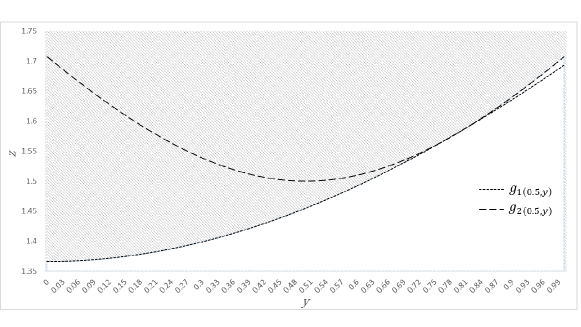
Figure 1. Functions $g_{1}$, $g_{2}$ with $\sigma=d=1$, $c=2$ ($x=0.5$).

Unfortunately, Proposition 7 does not help to describe the convex hull of $H_{\mathbb{G}}$ with more than one bounded variable. Additionally, piecewise valid functions like $g(x,y)$ in Proposition 7 cannot be directly used with standard algorithms for convex mixed-integer optimization. Thus, we now turn our attention to deriving inequalities that are valid and can be implemented as conic quadratic cuts, if not sufficient to describe $\text{conv}(H_{\mathbb{G}})$ in general.

5.2. The general (multi-variable) case

To obtain valid inequalities for $H_{\mathbb{G}}$ we write the conic quadratic constraint in extended form for a subset $T\subseteq M$ of the continuous variables:

$${s^{2}+\sum_{i\in M\setminus T}d_{i}y_{i}^{2}}\leq z^{2}$$

$${\sigma+}\sum_{i\in N}c_{i}x_{i}+\sum_{i\in T}d_{i}y_{i}^{2}\leq s^{2}.$$ (26)

$$x\in\{0,1\}^{n},y\in[0,1]^{M},s\geq 0.$$

Applying inequality (11) to (26) and eliminating the auxiliary variable $s$, we obtain the inequalities

$${\left(\sqrt{\sigma+\sum_{i\in T}d_{i}y_{i}^{2}}+\pi^{\prime}x\right)^{2}+\sum_{i\in M\setminus T}d_{i}y_{i}^{2}}\leq z^{2},\quad\pi\in\Pi_{\sigma+d(T)}.$$ (27)

Proposition 8.

For $T\subseteq M$ inequalities (27) are valid for $H_{\mathbb{G}}$.

Note that inequalities (27) generalize or strengthen the previous valid inequalities proposed in this paper and other inequalities in the literature.

Remark 5.

For $T=\emptyset$ inequalities (27) coincide with inequalities (13). For $T=M$ inequalities (27) coincide with inequalities (11). If $T\subset M$, then inequalities (27) dominate inequalities (11).

Example 1 (Continued).

We obtain from $\eqref{eq:polymatroidBounded}$ the valid inequality

$$g_{3}(x,y)=\sqrt{\sigma+dy^{2}}+x\left(\sqrt{\sigma+c+d}-\sqrt{\sigma+d}\right)\leq z$$

for $L$. As Figure 2 shows, the inequality provides a good approximation of $L$ for the example considered.

Figure 2. Functions $g_{1}$, $g_{2}$, $g_{3}$ with $\sigma=d=1$, $c=2$ $(x=0.5)$.

6. Valid inequalities for general $H_{X}$

In this section we derive inequalities that exploit the structure for an arbitrary set $X\subseteq{\mathbb{D}}$. We first describe a lifting procedure for obtaining valid inequalities for any mixed-binary set $X$, where computing each coefficient requires solving an integer optimization problem (Section 6.1). Then, we propose an approach based on linear programming to efficiently compute weaker valid inequalities (Section 6.2).

6.1. General mixed-binary set $X$

We now consider valid inequalities for $H_{X}$ where $X\subseteq{\mathbb{D}}$. The inequalities described here have a structure similar to the nonlinear extended polymatroid inequalities (13) and (27). For a given a permutation $\left((1),(2),\ldots,(n)\right)$ of $N$ and $T\subseteq M$, let

$$h_{k}(x,y) =\sigma+\sum_{i=1}^{k-1}c_{(i)}x_{(i)}+\sum_{i\in T}d_{i}y_{i}^{2}$$

$$\bar{\sigma}_{(k)} =\max\left\{h_{k}(x,y):(x,y)\in X,x_{k}=1\right\},\text{ and}$$ (28)

$$\rho_{(k)} =\begin{cases}\sqrt{c_{(k)}+\bar{\sigma}_{(k)}}-\sqrt{\bar{\sigma}_{(k)}}&\text{if }\bar{\sigma}_{(k)}<\infty\\ 0&\text{otherwise.}\end{cases}$$ (29)

Consider the inequality

$${\left(\sqrt{\sigma+\sum_{i\in T}d_{i}y_{i}^{2}}+\sum_{i=1}^{n}\rho_{(i)}x_{(i)}\right)^{2}+\sum_{i\in M\setminus T}d_{i}y_{i}^{2}}\leq z^{2}.$$ (30)

Proposition 9.

For $T\subseteq M$ inequalities (30) are valid for $H_{X}$.

Proof.

Let

$$H_{X}(T)=\left\{(x,y)\in X,s\geq 0:\sqrt{\sigma+\sum_{i\in N}c_{i}x_{i}+\sum_{i\in T}d_{i}y_{i}^{2}}\leq s\right\},$$

and consider the extended formulation of $H_{X}$ given by

$$\hat{H}_{X}=\left\{(x,y,s)\in H_{X}(T),z\geq 0:\sqrt{s^{2}+\sum_{i\in M\setminus T}d_{i}y_{i}^{2}}\leq z\right\}.$$

To prove the validity of (30) for $H_{X}$, it is sufficient to show that

$$\sqrt{\sigma+\sum_{i\in T}d_{i}y_{i}^{2}}+\sum_{i=1}^{n}\rho_{(i)}x_{(i)}\leq s$$ (31)

is valid for $H_{X}(T)$. In particular, we prove by induction that

$$\sqrt{\sigma+\sum_{i\in T}d_{i}y_{i}^{2}}+\sum_{i=1}^{k}\rho_{(i)}x_{(i)}\leq\sqrt{\sigma+\sum_{i=1}^{k}c_{(i)}x_{(i)}+\sum_{i\in T}d_{i}y_{i}^{2}}$$ (32)

for all $(x,y)\in X$ and $k=0,\ldots,n$.

Base case: $k=0$

Inequality (32) holds trivially.

Inductive step

Let $(\bar{x},\bar{y})\in X$, and suppose inequality (32) holds for $k-1$. Observe that if $\bar{x}_{(k)}=0$ or $\rho_{(k)}=0$, then inequality (32) clearly holds for $k$. Therefore, assume that $\bar{x}_{(k)}=1$ and $\bar{\sigma}_{(k)}<\infty$. We have

$$\sqrt{\sigma+\sum_{i=1}^{k}c_{(i)}\bar{x}_{(i)}+\sum_{i\in T}d_{i}\bar{y}_{i}^{2}} =\sqrt{h_{k}(\bar{x},\bar{y})+c_{(k)}}$$

$$=\sqrt{h_{k}(\bar{x},\bar{y})}+\left(\sqrt{h_{k}(\bar{x},\bar{y})+c_{(k)}}-\sqrt{h_{k}(\bar{x},\bar{y})}\right)$$

$$\geq\sqrt{h_{k}(\bar{x},\bar{y})}+\left(\sqrt{\bar{\sigma}_{(k)}+c_{(k)}}-\sqrt{\bar{\sigma}_{(k)}}\right)$$ (33)

$$\geq\sqrt{\sigma+\sum_{i\in T}d_{i}\bar{y}_{i}^{2}}+\sum_{i=1}^{k}\rho_{(i)}\bar{x}_{(i)},$$ (34)

where (33) follows from $\bar{\sigma}_{(k)}\geq h_{k}(\bar{x},\bar{y})$ (by definition of $\bar{\sigma}_{(k)}$) and from the concavity of the square root function, and (34) follows from $\sqrt{h_{k}(\bar{x},\bar{y})}\geq\sqrt{\sigma+\sum_{i\in T}d_{i}\bar{y}_{i}^{2}}+\sum_{i=1}^{k-1}\rho_{(i)}\bar{x}_{(i)}$ (induction hypothesis) and from the definition of $\rho_{(k)}$. ∎

Remark 6.

Note that $\sigma_{(k-1)}=\sigma+\sum_{i=1}^{k-1}c_{(i)}$ and, if $T=\emptyset$, then

$$\bar{\sigma}_{(k)}=\max_{\begin{subarray}{c}x\in X\\ x_{(k)}=1\end{subarray}}\sigma+\sum_{i=1}^{k-1}c_{(i)}x_{i}.$$

In particular, if $T=\emptyset$, then $\bar{\sigma}_{(k)}\leq\sigma_{(k-1)}$ and $\rho_{(k)}\geq\pi_{(k)}$. Thus, for $T=\emptyset$ and $X={\mathbb{D}}$, inequalities (30) reduce to inequalities (13); for $T=\emptyset$ and $X\subset{\mathbb{D}}$, inequalities (30) dominate inequalities (13).

Remark 7.

For $X={\mathbb{G}}$, inequalities (30) reduce to inequalities (27). For $X\subset{\mathbb{G}}$, inequalities (30) dominate inequalities (27).

Remark 8.

For the case of the pure-binary set with defined by a cardinality constraint, i.e., $Y=\left\{x\in\{0,1\}^{n}:\sum_{i=1}^{n}x_{i}\leq k\right\}$ and $\sigma=0$, Yu and Ahmed, (2017) give facets for conv$(H_{Y})$. However, noting the computation burden of constructing them, they propose approximate lifted inequalities of the form $\sum_{i\leq k}\pi_{(i)}x_{(i)}+\sum_{i>k}\rho_{(i)}x_{(i)}\leq z$, where $\pi$ are computed according to (9), and

$$\rho_{(i)}=\sqrt{c(T_{(i)})+c_{(i)}}-\sqrt{c(T_{(i)})}$$

with $T_{(i)}={\arg\max}\left\{c(T):T\subseteq\{(1),\ldots,(i-1)\},\;|T|=k-1\right\}.$ Thus, their approximate lifted inequalities coincide with inequalities (30) and can be computed in $O(n\log n)$. If the set $X$ has additional constraints, then inequalities (30) are stronger than the approximate lifted inequalities of Yu and Ahmed, (2017).

Remark 9.

The strengthened extended polymatroid inequalities described in this section can be used with rotated cone constraints as well. In particular, for the set

$$R_{X}=\left\{(x,y)\in X,w\geq 0,z\geq 0:\sigma+\sum_{i\in N}c_{i}x_{i}+\sum_{i\in M}d_{i}y_{i}^{2}\leq 4wz\right\},$$

we find that inequalities

$$\left(\sqrt{\sigma+\sum_{i\in T}d_{i}y_{i}^{2}}+\sum_{i=1}^{n}\rho_{(i)}x_{(i)}\right)^{2}+\sum_{i\in M\setminus T}d_{i}y_{i}^{2}\leq 4wz$$ (35)

are valid for $R_{X}$.

6.2. Relaxed inequalities

Note that computing each coefficient of inequality (30) requires solving a non-convex mixed 0-1 optimization problem (28), which may not be practical in most cases. However, observe from Remarks 6 and 7 that solving the optimization problem over any relaxation of $X$ that includes the bound constraints results in valid inequalities at least as strong as the ones resulting from using only the bound constraints.

In particular, assume in problem (28) that, for $i\in T$, $y_{i}$ has a finite upper bound (otherwise the problem is unbounded and $\rho_{i}=0$) and $u_{i}=1$ (by scaling). Moreover let $X_{P}$ be a polyhedron such that $X\subseteq X_{P}$. Convex constraints can also be included in $X_{P}$ by using a suitable linear outer approximation (Ben-Tal and Nemirovski, 2001, Tawarmalani and Sahinidis, 2005, Hijazi et al., 2013, Lubin et al., 2016).

Given $X_{P}$, the approximate coefficients

$$\hat{\rho}_{(k)} =\sqrt{c_{(k)}+\hat{\sigma}_{(k)}}-\sqrt{\hat{\sigma}_{(k)}}\text{, with}$$ (36)

$$\hat{\sigma}_{(k)} =\sigma+\max\left\{\sum_{i=1}^{k-1}c_{(i)}x_{(i)}+\sum_{i\in T}d_{i}y_{i}:(x,y)\in X_{P},x_{k}=1\right\}$$

can be computed efficiently by solving $n$ linear programs. Moreover, the linear program required to compute $\hat{\sigma}_{(k)}$ differs from the one required for $\hat{\sigma}_{(k-1)}$ in two bound constraints, corresponding to $x_{(k-1)}$ and $x_{(k)}$, and one objective coefficient, corresponding to $x_{(k-1)}$. Therefore, using the simplex method with warm starts, each $\hat{\sigma}_{(k)}$ can be computed efficiently, using only a small number of simplex pivots.

7. Computational considerations

Table 1 presents a classification of the proposed inequalities, depending on whether the continuous variables are bounded or not, on whether the inequalities are for the set with the conic quadratic cone $H_{X}$ or the rotated cone $R_{X}$, and on whether additional constraints are used to strengthen the inequalities (strengthened) or not (polymatroid). Note that there is a direct correspondence between the inequalities for conic quadratic cones and for rotated cones and, although not explicitly shown in the paper, it is easy to construct the rotated cone version of inequality (27).

Table 1. Classification of the proposed inequalities.

Continuous variables	polymatroid		strengthened
	conic quad	rotated	conic quad	rotated
Unbounded	(13)	(17)	(30), $T=\emptyset$	(35), $T=\emptyset$
Bounded	(27)		(30)	(35)

We now consider the implementation of the proposed inequalities in branch-and-cut algorithms. First, in Section 7.1, we discuss the difficulties in using the inequalities for the (more general) bounded case, then in Section 7.2 we show how to efficiently use the cuts for the unbounded case.

7.1. Bounded case

For brevity, we only discuss inequalities (27) of the form $\varphi(x,y)\leq z$, where

$$\varphi(x,y)=\sqrt{\left(\sqrt{\sigma+\sum_{i\in T}d_{i}y_{i}^{2}}+\pi^{\prime}x\right)^{2}+\sum_{i\in M\setminus T}d_{i}y_{i}^{2}}.$$

All other inequalities for the bounded case have a similar structure, so the discussion extends directly to those cases as well. Inequalities (27) are nonlinear, and can be added to the formulation as nonlinear inequalities, or can be implemented via linear cutting planes using outer approximations. Unfortunately, both approaches have drawbacks which may limit the effectiveness of the inequalities in practice when used with current off-the-shelf solvers.

7.1.1. Implementation as nonlinear cuts

The function $\varphi$ is conic quadratic-representable; in particular, the inequality $\varphi(x,y)\leq z$ is equivalent to the system

$$s_{1}^{2} \geq\sigma+\sum_{i\in T}d_{i}y_{i}^{2}$$ (37)

$$s_{2} =s_{1}+\pi^{\prime}x$$

$$z \geq s_{2}^{2}+\sum_{i\in M\setminus T}d_{i}y_{i}^{2}$$ (38)

$$0 \leq s_{1},s_{2},$$

where (37) and (38) are conic quadratic inequalities accepted by most solvers.

Observe that adding each inequality (27) requires two additional variables and conic constraints, thus adding even a modest number of inequalities may substantially increase the difficulty of solving the convex relaxations at each node of the branch-and-bound tree. Additionally, solvers rely on the dual simplex method to solve the subproblems arising in branch-and-bound (by constructing a linear approximation of non-polyhedral sets) due to its warm starts capabilities; adding nonlinear cuts such as (37) and (38) may render the existing simplex tableau ineffective and require solving the subproblems from scratch. Finally, commercial solvers, currently, do not allow adding nonlinear cuts during branching, and inequalities (27) need to be added by the user at the root node explicitly, giving up the benefits of built-in cut-management strategies.

7.1.2. Implementation as linear outer approximations

Cutting planes based on a linear outer approximation of the convex function $\varphi$ can be added using gradients. Given a fractional solution $(\bar{x},\bar{y})$, the linear underestimator $\bar{\varphi}(x,y)\leq z$, where

$$\bar{\varphi}(x,y)=\varphi(\bar{x},\bar{y})+\nabla_{x}\varphi(\bar{x})^{\prime}(x-\bar{x})+\nabla_{y}\varphi(\bar{y})^{\prime}(y-\bar{y})$$

is valid. In particular, we find

$$\bar{\varphi}(x,y)=\psi+\frac{1}{\psi}\left(\eta\pi^{\prime}(x-\bar{x})+\zeta\sum_{i\in T}d_{i}\bar{y}_{i}(y_{i}-\bar{y}_{i})+\sum_{i\in M\setminus T}d_{i}\bar{y}_{i}(y_{i}-\bar{y}_{i})\right),$$

where

$$\eta=\sqrt{\sigma+\sum_{i\in T}d_{i}\bar{y}_{i}^{2}}+\pi^{\prime}\bar{x};\ \ \zeta=\frac{\eta}{\sqrt{\sigma+\sum_{i\in T}d_{i}\bar{y}_{i}^{2}}};\ \ \psi=\sqrt{\eta^{2}+\sum_{i\in M\setminus T}d_{i}\bar{y}_{i}^{2}}.$$

An implementation based on the linear cuts $\bar{\varphi}(x,y)\leq z$ leverages the existing capabilities of current commercial solvers, including warm starts and cut management strategies. Nevertheless, each linear inequality $\bar{\varphi}(x,y)\leq z$ is often weak, and constructing a suitable approximation of the original nonlinear inequality $\varphi(x,y)\leq z$ may require a prohibitive number of cuts.

In Appendix B we provide a comparison of both approaches for a simple mean-risk minimization problem with bounded continuous variables and no correlations. Adding the nonlinear inequalities directly, as discussed in Section 7.1.1, results in significantly better performance, both in terms of the relaxation quality and the solution times. These results are consistent with the recent experience by the authors using other classes of nonlinear inequalities, see Atamtürk and Gómez, (2018) and Gómez, (2018).

7.2. Unbounded case

In most of the applications discussed in Section 2, the continuous variables are used to model covariance terms, rotated cone constraints or denominators in fractional optimization. In such cases, the continuous variables are unbounded, and the proposed inequalities can be implemented efficiently in such settings. Observe that the conic quadratic inequality arising in set $H_{X}$ can be written in an extended formulation as

$$s^{2} \geq\sum_{i\in N}c_{i}x_{i}^{2}$$

$$z^{2} \geq s^{2}+\sum_{i\in M}d_{i}y_{i}^{2}$$

$$0 \leq s.$$

Similarly, the rotated cone inequality arising in set $R_{X}$ can be written as

$$s^{2} \geq\sum_{i\in N}c_{i}x_{i}^{2}$$

$$t^{2} \geq s^{2}+\sum_{i\in M}d_{i}y_{i}^{2}$$

$$t^{2} \leq wz$$

$$0 \leq s,t.$$

In both cases, the polymatroid and strengthened inequalities can be added as linear cuts, $\pi^{\prime}x\leq s$ and $\rho^{\prime}x\leq s$, respectively. Thus, when adding the nonlinear inequalities as linear cuts in an extended formulation, optimization algorithms benefit from the warm starts and cut management strategies without sacrificing the strength of the inequalities. Such a formulation cannot be used effectively for the bounded case, since an additional variable would be needed for each subset $T$ of $M$.

8. Experiments

In this section we report computational experiments performed to test the effectiveness of the polymatroid inequalities in solving second order cone optimization with a branch-and-cut algorithm. In Section 8.1 we solve instances with general covariance matrices (see application in Section 2.2), in Section 8.2 we solve conic quadratic interdiction problems (see application in Section 2.3), and in Section 8.3 we solve binary linear fractional problems (see applications in Section 2.6).

All experiments are done using CPLEX 12.6.2 solver on a workstation with a 2.93GHz Intel®Core^TM i7 CPU and 8 GB main memory and with a single thread. We compare using default CPLEX without adding any cuts (cpx), using the inequalities in Section 4 (polymatroid) and using the strengthened inequalities in Section 6 (strengthened). Since in all cases the continuous variables are unbounded, we implement the inequalities as discussed in Section 7.2. The time limit is set to two hours and CPLEX’ default settings are used. The inequalities are added only at the root node using callback functions, and all times reported include the time required to add cuts.

8.1. Mean-risk minimization with correlated random variables

In this section we test the effectiveness of the polymatroid inequalities in instances with correlated random variables. In particular, we solve mean-risk minimization problems

$$\min_{x\in\{0,1\}^{n}}\left\{-a^{\prime}x+\Omega\sqrt{x^{\prime}Qx}:\sum_{i=1}^{n}x_{i}\leq k\right\},$$ (39)

where the matrix $Q$ is generated according to a factor model, i.e., $Q={Z}F{Z}^{\prime}+D$ where $F\in\mathbb{R}^{r\times r}$ is the factor covariance matrix, ${Z}\in\mathbb{R}^{n\times r}$ is the exposure matrix and $D\in\mathbb{R}^{n\times n}$ is diagonal matrix with the specific covariances. Observe that in such instances, we can set $\text{diag}(c)=D$ in equation (2.2).

In our experiments $F=GG^{\prime}$, with $G\in\mathbb{R}^{r\times r}$ and $G_{ij}\sim U[-1,1]$, ${Z}_{ij}\sim U[0,1]$ with probability $0.2$ and ${Z}_{ij}=0$ otherwise, $D_{ii}\sim U[0,\delta\bar{q}]$, where $\delta\geq 0$ is a diagonal dominance parameter and $\bar{q}=\frac{1}{N}\sum_{i\in N}{Q_{0}}_{ii}$, and $a_{i}\sim U[0.85\sqrt{Q_{ii}},1.15\sqrt{Q_{ii}}]$. We set the parameter $\Omega=\Phi^{-1}(\alpha)$, where $\Phi$ is the cumulative distribution function of the normal distribution and $\alpha\in\{0.95,0.975,0.99\}$. We let $n=200$, $r=40$ and $k$ equal to 10%, 15%, and 20% of the number of the variables.

Table 2. Experiments with general covariance matrices ($\delta=0.5$).

$k$	$\alpha$	igap	cpx				polymatroid				strengthened
			rimp	nodes	time	egap[#]	rimp	nodes	time	egap[#]	rimp	nodes	time	egap[#]
20	0.95	1.7	22.6	9,557	74	0.0[5]	53.3	3,957	23	0.0[5]	55.6	2,367	17	0.0[5]
	0.975	3.0	21.3	33,468	242	0.0[5]	53.5	13,316	86	0.0[5]	55.9	5,839	40	0.0[5]
	0.99	5.2	15.2	164,568	1,845	0.0[5]	52.8	80,735	730	0.0[5]	55.3	23,577	269	0.0[5]
Average			19.7	69,198	720	0.0[15]	53.2	32,669	280	0.0[15]	55.6	10,594	109	0.0[15]
30	0.95	0.8	15.5	7,115	57	0.0[5]	53.3	1,656	11	0.0[5]	52.4	1,159	9	0.0[5]
	0.975	1.3	14.9	18,901	135	0.0[5]	53.1	2,800	20	0.0[5]	54.0	2,095	15	0.0[5]
	0.99	2.3	5.7	76,675	1,005	0.0[5]	61.1	8,265	48	0.0[5]	62.1	5,131	30	0.0[5]
Average			12.0	34,230	399	0.0[15]	55.8	4,240	26	0.0[15]	56.2	2,795	18	0.0[15]
40	0.95	0.4	23.3	2,910	18	0.0[5]	48.5	611	6	0.0[5]	50.5	577	6	0.0[5]
	0.975	0.7	20.0	4,216	30	0.0[5]	54.3	884	7	0.0[5]	55.5	839	7	0.0[5]
	0.99	1.1	13.5	46,030	514	0.0[5]	55.9	2,493	18	0.0[5]	56.7	2,144	14	0.0[5]
Average			18.9	17,719	187	0.0[15]	52.9	1,329	10	0.0[15]	54.2	1,187	9	0.0[15]

Table 3. Experiments with general covariance matrices ($\delta=1.0$).

$k$	$\alpha$	igap	cpx				polymatroid				strengthened
			rimp	nodes	time	egap[#]	rimp	nodes	time	egap[#]	rimp	nodes	time	egap[#]
20	0.95	2.9	21.6	64,283	927	0.0[5]	55.1	14,984	165	0.0[5]	59.1	6,233	68	0.0[5]
	0.975	5.0	15.5	240,224	3,975	0.4[3]	44.4	189,826	3,390	0.4[3]	50.9	102,053	1,915	0.1[4]
	0.99	9.0	6.4	378,116	7,200	2.2[0]	35.7	477,553	7,200	1.9[0]	43.1	430,707	5,966	0.6[2]
Average			14.5	227,541	4,034	0.9[8]	45.1	227,454	3,585	0.8[8]	51.0	179,664	2,650	0.2[11]
30	0.95	1.1	17.1	32,629	316	0.0[5]	77.2	1,082	12	0.0[5]	78.2	682	10	0.0[5]
	0.975	2.0	12.5	150,756	2,046	0.1[4]	72.9	12,202	107	0.0[5]	75.5	4,896	39	0.0[5]
	0.99	3.5	10.5	258,866	3,679	0.5[3]	67.8	115,507	1,510	0.1[4]	70.6	59,106	511	0.0[5]
Average			13.4	147,417	2,014	0.2[12]	72.6	42,930	543	0.0[14]	74.8	21,561	187	0.0[15]
40	0.95	0.6	23.9	6,522	64	0.0[5]	72.3	270	9	0.0[5]	74.8	192	8	0.0[5]
	0.975	1.0	24.0	31,022	414	0.0[5]	71.0	823	12	0.0[5]	72.1	695	11	0.0[5]
	0.99	1.6	17.6	122,568	2,907	0.2[3]	73.9	4,416	37	0.0[5]	75.1	2,543	26	0.0[5]
Average			21.8	53,371	1,128	0.1[13]	72.4	1,836	19	0.0[15]	74.0	1,143	15	0.0[15]

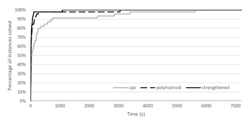
(a) $\delta=0.5$.

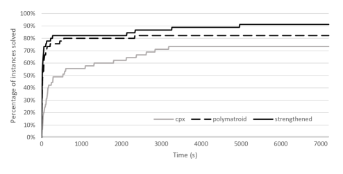
(b) $\delta=1.0$.

Figure 3. Percentage of instances solved within a given time limit for mean-risk minimization with correlated random variables.

Tables 2 and 3 present the results for different values of the diagonal dominance parameter $\delta$. Each row represents the average over five instances generated with the same parameters and shows the initial gap (igap), the root gap improvement (rimp), the number of nodes explored (nodes), the time elapsed in seconds (time), and the end gap (egap)[in brackets, the number of instances solved to optimality (#)]. The initial gap is computed as $\texttt{igap}=\frac{t_{\text{opt}}-t_{\text{relax}}}{\left|t_{\text{opt}}\right|}\times 100$, where $t_{\text{opt}}$ is the objective value of the best feasible solution at termination and $t_{\text{relax}}$ is the objective value of the continuous relaxation. The end gap is computed as $\texttt{egap}=\frac{{t_{\text{opt}}}-t_{\text{bb}}}{\left|t_{\text{opt}}\right|}\times 100$, where $t_{\text{bb}}$ is the objective value of the best lower bound at termination. The root improvement is computed as $\texttt{rimp}=\frac{t_{\text{root}}-t_{\text{relax}}}{t_{\text{opt}}-t_{\text{relax}}}\times 100$, where $t_{\text{root}}$ is the value of the continuous relaxation after adding the valid inequalities to the formulation. Figure 3 shows the corresponding performance profiles.

Observe that adding inequalities polymatroid or strengthened closes the initial integrality gaps by 45% to 75%, resulting in significant performance improvement over default CPLEX. In particular, using inequalities strengthened for instances with $k=20$ leads to seven times speed-up with $\delta=0.5$ and two times speed-up with $\delta=1$) and lower end gaps. Moreover, for instances with $k\geq 30$ using inequalities strengthened results in at least an order-of-magnitude speed-up over default CPLEX. The impact of both inequalities increases with higher diagonal dominance as expected. In Figure 3 we see that for $\delta=1.0$ cpx requires close to 3,000 seconds to solve 70% of the instances, while polymatroid requires 110 seconds and strengthened requires 50 seconds to solve a similar number of instances, i.e., strengthened is 50 times faster than cpx; in fact, strengthened solves in 60 seconds 73% of the instances, the same quantity that cpx solves in 2 hours. Finally, we see that the strengthened inequalities result in consistently better performance than the simpler polymatroid inequalities .

8.2. Conic quadratic interdiction instances

In this section we test the effectiveness of the proposed inequalities for the interdiction problem (CQI) discussed in Section 2.3. In our computations, we model a decision-maker that seeks a path with minimal value-at-risk. After the decision-maker decides on a path, an adversary may attack a limited number of arcs on the path, increasing the expectation and/or covariance of travel times/costs.

The feasible region $X$ is given by path constraints on a $40\times 40$ grid network. There is a potential adverse event corresponding to each arc, and each event results in an increase in the nominal duration/cost and variance of that arc: in particular, for $i=1,\ldots,n$, $a_{i}\sim U[0,2]e^{i}$, where $e^{i}$ is the vector which has value $1$ in the $i$-th position and $0$ elsewhere, and the $i$-th row and column of $Q_{i}$ is drawn from $U[0,2]$ and $Q_{i}$ has 0 entries elsewhere. Each element of the nominal cost vector $a_{0}$ is drawn from $U[0,1]$, and the squared roots of every diagonal element of $Q_{0}$ are also generated from $U[0,1]$. The parameter $\Omega$ is set as in Section 8.1.

Table 4 shows the results for different values of $\alpha$ and the parameter controlling the number of attacks $\Gamma$, and Figure 4 shows the corresponding performance profile. Observe that the strengthened cuts result in a better root improvement of 55% – compared to 30–37% achieved by default CPLEX. Moreover, when using the strengthened inequalities, 37 instances are solved to optimality, while default CPLEX is able to solve only 22 instances. We also see that in these path instances, the polymatroid inequalities result in longer solution times than cpx (despite better root improvements). On the other hand, the strengthened inequalities are effective both in reducing the integrality gaps and solution times.

Table 4. Experiments with robust conic instances.

${\Gamma}$	$\alpha$	igap	cpx				polymatroid				strengthened
			rimp	nodes	time	egap[#]	rimp	nodes	time	egap[#]	rimp	nodes	time	egap[#]
4	0.95	22.6	35.1	65,533	3,124	0.6[4]	44.3	72,322	5,220	1.2[3]	56.8	17,057	917	0.0[5]
	0.975	24.1	30.2	95,337	4,239	0.8[4]	41.1	87,697	7,200	3.5[0]	55.2	53,022	2,648	0.0[5]
	0.99	25.7	26.6	153,481	7,200	2.2[0]	37.9	80,160	7,200	7.6[0]	53.5	102,578	4,452	0.0[5]
Average			30.6	104,117	4,854	1.2[8]	41.1	80,060	6,540	4.1[3]	55.2	57,552	2,672	0.0[15]
6	0.95	26.9	38.8	73,898	3,422	0.4[4]	45.0	89,319	5,771	2.0[3]	56.2	33,364	1,644	0.0[5]
	0.975	28.1	34.6	138,231	5,676	1.8[2]	41.3	96,917	7,200	5.5[0]	54.1	113,745	4,895	0.0[5]
	0.99	29.7	32.0	160,074	6,823	4.2[1]	38.9	94,762	7,200	7.2[0]	52.2	113,954	6,091	2.0[1]
Average			35.1	124,068	5,307	2.1[7]	41.7	93,666	6,704	4.9[2]	54.2	87,021	4,210	0.7[11]
8	0.95	30.2	40.9	143,946	5,474	0.8[4]	46.4	112,279	6,822	1.6[1]	55.2	53,942	2,234	0.0[5]
	0.975	31.3	36.3	145,582	5,967	1.9[2]	42.7	107,432	7,200	4.8[0]	53.4	99,904	4,679	0.4[4]
	0.99	32.7	34.2	123,325	6,512	3.5[1]	39.5	94,691	7,200	8.2[0]	51.1	136,632	6,162	2.4[2]
Average			37.1	137,618	5,984	2.1[7]	42.8	104,801	7,055	4.9[1]	53.2	96,826	4,358	0.9[11]

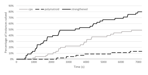
Figure 4. Percentage of instances solved within a given time limit for interdiction problems.

8.3. Binary fractional optimization instances

We now test the inequalities in a binary fractional problem arising in assortment optimization with cardinality constraint:

$$\text{(FP)}\ \ \max\left\{\sum_{j=1}^{m}\frac{\sum_{i=1}^{n}c_{ij}x_{i}}{a_{0j}+\sum_{i=1}^{n}a_{ij}x_{i}}\ :\ \sum_{i=1}^{n}x_{i}\leq k,\ x\in\{0,1\}^{n}\right\}\cdot$$

The data is generated as in the assortment optimization problems considered in Şen et al., (2015): $a_{ij}\sim U[0,1]$ for all $i,j$, $c_{ij}=a_{ij}r_{ij}$ with $r_{ij}\sim U[1,3]$, $n=200$, $m=20$ and $a_{0j}=a_{0}$ for all $j=1,\ldots,m$ with $a_{0}\in\{5,10\}$, and $k\in\{10,20,50\}$.

Binary fractional problems (FP) are usually solved by linearizing the fractional terms (see Tawarmalani et al., 2002, Prokopyev et al., 2005, Bront et al., 2009, Méndez-Díaz et al., 2014, Şen et al., 2015, Borrero et al., 2016b ), which requires the addition of $O(nm)$ additional variables and big-M constraints. On the other hand, the rotated cone reformulation outlined in Section 2.6, requires adding only $m$ additional variables and avoids big-M constraints altogether.

We test the classical big-M linear formulation used in Bront et al., (2009), Méndez-Díaz et al., (2014) (cpx-milo), the conic formulation without adding inequalities (cpx-conic) and the conic formulation strengthened with polymatroid inequalities . Table 5 shows the results. Each row represents the average over five instances generated with the same parameters and for each combination of the parameters $a_{0}$ and $k$ and for each formulation, the root gap (rgap), the number of nodes explored (nodes), the time elapsed in seconds (time), and the end gap (egap)[in brackets, the number of instances solved to optimality (#)]. The root gap is computed as $\texttt{rgap}=\frac{t_{\text{opt}}-t_{\text{root}}}{\left|t_{\text{opt}}\right|}\times 100$, where $t_{\text{opt}}$ is the objective value of the best feasible solution at termination, and $t_{\text{root}}$ is the objective value of the relaxation obtained after processing the root node (i.e., after user cuts and cuts added by CPLEX).

Table 5. Experiments with binary fractional optimization.

$a_{0}$	$k$	cpx-milo				cpx-conic				polymatroid
		rgap	nodes	time	egap[#]	rgap	nodes	time	egap[#]	rgap	nodes	time	egap[#]
5	10	50.9	20,737	7,200	43.6[0]	3.1	24,073	572	0.0[5]	0.1	46	19	0.0[5]
	20	18.0	51,180	7,200	17.0[0]	2.7	123,655	7,200	1.9[0]	0.0	118	54	0.0[5]
	50	0.9	621,742	6,010	0.5[1]	4.9	55,155	7,200	4.5[0]	0.1	15,465	263	0.0[5]
Average		23.3	231,220	6,803	20.4[1]	3.2	67,628	4,991	2.1[5]	0.1	5,210	112	0.0[15]
10	10	46.8	380,700	7,200	15.9[0]	2.2	48,541	972	0.0[5]	0.0	6	14	0.0[5]
	20	39.8	23,770	7,200	37.4[0]	3.7	206,603	7,200	1.4[0]	0.0	61	37	0.0[5]
	50	5.6	136,382	7,200	5.2[0]	5.1	52,700	7,200	4.6[0]	0.1	36,959	396	0.0[5]
Average		30.7	180,284	7,200	19.5[0]	4.3	102,615	5,124	2.0[5]	0.0	12,342	149	0.0[15]

We see that the conic formulation with polymatroid inequalities results in substantially faster solution times than the other formulations. In particular, CPLEX with the classical big-M linear optimization formulation cpx-milo can only solve 1/30 instances after two hours of branch and bound, and the average end gaps are 20%; the conic formulation with extended polymatroid cuts is able to solve all instances to optimality in less than 3 minutes (on average). We see that root gaps for polymatroid are very small in all instances (less than 0.1%), and optimality can be proven in instances with small cardinality parameter $k$ after few branch-and-bound nodes (e.g., in instances with $k=10$ and $a_{0}=5$ optimality is proven after 46 nodes, while cpx-conic requires 24,000 nodes to prove optimality).

9. Conclusions

We propose new convex valid inequalities that exploit submodularity for conic quadratic mixed 0-1 sets. The studied sets arise in a variety of risk-adverse decision-making problems (e.g, chance constrained optimization with correlated variables, robust optimization with ellipsoidal or discrete uncertainty sets) as well as in models of other problems commonly arising in operations research (e.g., lot sizing, scheduling, assortment, fractional linear optimization). The unbounded version of the convex inequalities, which arise naturally in most applications, can be efficiently implemented as linear cuts in an extended space, which make them particularly effective. Moreover, the inequalities can be strengthened to take advantage of other constraints in a problem through approximate lifting without affecting this convenient property. Computational experiments performed on correlated mean-risk minimization, robust interdiction and assortment optimization problems indicate that the proposed inequalities improve the performance of branch-and-bound solvers substantially; in some cases, problems for which no efficient algorithms were known are now solved in seconds.

Appendix A

Proof of Proposition 6.

Consider the optimization of an arbitrary linear function over the convex relaxation of the extended formulation of $U_{R}$ given by:

$$\ \ \ \ \ \ \ \min\; a^{\prime}x+b^{\prime}y+pw+qz$$

($$P_{R} {s^{2}+\sum_{i\in M}d_{i}y_{i}^{2}+(w-z)^{2}}\leq(w+z)^{2}$$)s.t. (40)

$$(x,s)\in\text{conv}({U_{0}})$$

$$y\in\mathbb{R}_{+}^{m},w\geq 0,z\geq 0.$$

Without loss of generality, we can assume that $p>0$ and $q>0$ (if $p<0$ or $q<0$ then the problem is unbounded, and if $p=0$ or $q=0$ then ($P_{R}$) reduces to a linear program over an integral polyhedron). Moreover, observe that if $w=z$ in an optimal solution, then the problem reduces to a linear optimization over ${\text{conv}(}U{)}$ which has an optimal integral solution (Proposition 5). Thus, we can assume that $w\neq z$, in which case the left hand size of (40) is differentiable, and we infer from KKT conditions with respect to $w$ and $z$ that

$$-p =-\lambda+\lambda\frac{w-z}{\sqrt{s^{2}+\sum_{i\in M}d_{i}y_{i}^{2}+(w-z)^{2}}}$$ (41)

$$-q =-\lambda-\lambda\frac{w-z}{\sqrt{s^{2}+\sum_{i\in M}d_{i}y_{i}^{2}+(w-z)^{2}}},$$ (42)

where $\lambda$ is the dual variable associated with constraint (40). We deduce from (41) that $w-z=\frac{\lambda-p}{\lambda}\sqrt{s^{2}+\sum\limits_{i\in M}d_{i}y_{i}^{2}+(w-z)^{2}}$, and from (42) that

$$w-z=\frac{q-\lambda}{\lambda}\sqrt{s^{2}+\sum\limits_{i\in M}d_{i}y_{i}^{2}+(w-z)^{2}}.$$ (43)

In particular, we find that $\lambda=\frac{p+q}{2}.$

Moreover, we obtain from (43) that

$$(w-z)^{2} =\left(\frac{q-\lambda}{\lambda}\right)^{2}\left(s^{2}+\sum_{i\in M}d_{i}y_{i}^{2}+(w-z)^{2}\right)$$

$$=\left(\frac{q-p}{q+p}\right)^{2}\left(s^{2}+\sum_{i\in M}d_{i}y_{i}^{2}+(w-z)^{2}\right).$$

Letting $\beta=\frac{\left(\frac{q-p}{q+p}\right)^{2}}{1-\left(\frac{q-p}{q+p}\right)^{2}}$, we deduce that

$$(w-z)^{2}=\beta\left(s^{2}+\sum_{i\in M}d_{i}y_{i}^{2}\right).$$

Therefore, we have that

$$\sqrt{s^{2}+\sum_{i\in M}d_{i}y_{i}^{2}+(w-z)^{2}}=\sqrt{1+\beta}\sqrt{s^{2}+\sum_{i\in M}d_{i}y_{i}^{2}}.$$

Moreover, since in any optimal solution of ($P_{R}$) constraint (40) is binding, we have

$$w+z=\sqrt{1+\beta}\sqrt{s^{2}+\sum_{i\in M}d_{i}y_{i}^{2}}.$$

Multiplying equality (41) by $w$ in both sides, and multiplying equality (42) by $z$ in both sides, we find that

$$pw+qz =\lambda(w+z)-\lambda\frac{(w-z)^{2}}{\sqrt{s^{2}+\sum_{i\in M}d_{i}y_{i}^{2}+(w-z)^{2}}}$$

$$=\lambda\sqrt{1+\beta}\sqrt{s^{2}+\sum_{i\in M}d_{i}y_{i}^{2}}-\lambda\frac{\beta\left(s^{2}+\sum_{i\in M}d_{i}y_{i}^{2}\right)}{\sqrt{1+\beta}\sqrt{s^{2}+\sum_{i\in M}d_{i}y_{i}^{2}}}$$

$$=\lambda\frac{s^{2}+\sum_{i\in M}d_{i}y_{i}^{2}}{\sqrt{1+\beta}\sqrt{s^{2}+\sum_{i\in M}d_{i}y_{i}^{2}}}$$

$$=\frac{\lambda}{\sqrt{1+\beta}}\sqrt{s^{2}+\sum_{i\in M}d_{i}y_{i}^{2}}.$$ (44)

Therefore, substituting $pw+qz$ in the objective function of ($P_{R}$) by (44) and using that $\lambda=\frac{p+q}{2}$, we see that problem ($P_{R}$) reduces to

$$\ \ \ \ \ \ \ \min\; a^{\prime}x+b^{\prime}y+\frac{p+q}{2\sqrt{1+\beta}}\sqrt{s^{2}+\sum_{i\in M}d_{i}y_{i}^{2}} P_{R}^{\prime}$$ ()

s.t. $$(x,s)\in\text{conv}(U_{0}),y\in\mathbb{R}_{+}^{m}.$$

Moreover, ($P_{R}^{\prime}$) is of the form of ($P_{2}$) in Proposition 5 (after scaling), thus has an optimal integer solution. Therefore, after projecting out the additional variable $s$, we find the desired result. ∎

Appendix B

In this section we test the effectiveness of the unbounded polymatroid inequalities (13) and bounded inequalities (27) in solving optimization problems with bounded continuous variables of the form

$$\min\left\{-a^{\prime}x-b^{\prime}y+\Omega z:(x,y,z)\in H_{\mathbb{G}}\right\}.$$ (45)

For two numbers $\ell<u$, let $U[\ell,u]$ denote the continuous uniform distribution between $\ell$ and $u$. The data for the model is generated as follows: $a_{i}\sim U[0,1]$, $\sqrt{c_{i}}\sim U[0.85a_{i},1.15a_{i}]$ for $i\in N$, $b_{j}\sim U[0,1]$, $\sqrt{d_{j}}\sim U[0.85b_{j},1.15b_{j}]$ for $j\in M$, and $\Omega$ is the solution of

$$-a(N)-b(M)+\Omega\sqrt{c(N)+d(M)}=0.$$

These instances have large integrality gaps with a single conic quadratic constraint.

The unbounded inequalities are added as linear cuts in an extended formulation, as described in Section 7.2. The bounded inequalities are either added directly as nonlinear inequalities as described in Section 7.1.1 (bounded-nonlinear), or using outer approximations as described in Section 7.1.2 (bounded-gradient). A greedy heuristic is used to choose $T\subseteq M$ for inequalities (27): given a fractional point $(\bar{x},\bar{y},\bar{z})$ with $\bar{y}_{(1)}\geq\bar{y}_{(2)}\geq\ldots\geq\bar{y}_{(m)}$, we check for violation inequalities for each $T_{i}$ of the form $T_{i}=\{(1),(2),\cdots,(i)\}$ for $i=0,\ldots,m$. When using the nonlinear inequalities bounded-nonlinear, we iteratively solve the continuous relaxations and explicitly add the most violated inequality (27) found, and the process is repeated until the relative violation of the inequality found is less than $10^{-3}$, i.e.,

$$\frac{\sqrt{\left(\sqrt{\sigma+\sum_{i\in T}d_{i}\bar{y}_{i}^{2}}+\pi^{\prime}\bar{x}\right)^{2}+\sum_{i\in M\setminus T}d_{i}\bar{y}_{i}^{2}}}{\bar{z}}-1\leq 10^{-3}.$$

Observe that this process requires solving many continuous relaxations of (45) using the barrier algorithm (which is the default algorithm for convex conic quadratic optimization). For bounded-gradient, the inequalities are added at the root node of the branch-and-bound tree using CPLEX callbacks.

Table 6 presents the results. Each row represents the average over five instances generated with the same parameters and shows the number of discrete ($n$) and continuous ($m$) variables, the initial gap (igap), the root gap improvement (rimp), the number of nodes explored (nodes), the time elapsed (including the time used adding the inequalities) in seconds (time), and the end gap (egap)[in brackets, the number of instances solved to optimality (#)]. The initial gap is computed as $\texttt{igap}=\frac{t_{\text{opt}}-t_{\text{relax}}}{\left|t_{\text{opt}}\right|}\times 100$, where $t_{\text{opt}}$ is the objective value of the best feasible solution at termination and $t_{\text{relax}}$ is the objective value of the continuous relaxation. The end gap is computed as $\texttt{egap}=\frac{{t_{\text{opt}}}-t_{\text{bb}}}{\left|t_{\text{opt}}\right|}\times 100$, where $t_{\text{bb}}$ is the objective value of the best lower bound at termination. The root improvement is computed as $\texttt{rimp}=\frac{t_{\text{root}}-t_{\text{relax}}}{t_{\text{opt}}-t_{\text{relax}}}\times 100$, where $t_{\text{root}}$ is the value of the continuous relaxation after adding the valid inequalities to the formulation.

Table 6. Experiments with bounded continuous variables.

$n$	$m$	igap	cpx				unbounded				bounded-gradient				bounded-nonlinear
			rimp	nodes	time	egap[#]	rimp	nodes	time	egap[#]	rimp	nodes	time	egap[#]	rimp	nodes	time	egap[#]
100	20	1,554.7	0.0	441,520	162	0.0[5]	90.0	9,617	112	0.0[5]	99.7	25	74	0.0[5]	100.0	1	45	0.0[5]
	50	724.6	0.0	2,126,713	1,644	0.0[5]	76.0	853,671	7,200	72.5[0]	99.2	1,985	4,375	0.0[5]	99.9	30	219	0.0[5]
	100	267.8	0.0	8,922,545	6,850	16.6[1]	62.1	726,361	7,200	83.3[0]	81.0	-	7,200	53.8[0]	99.9	55	84	0.0[5]
Average			0.0	3,830,259	2,885	5.6[11]	76.0	529,883	4,804	51.9[5]	93.3	670	3,874	17.9[10]	100.0	29	116	0.0[15]
200	40	987.1	0.0	15,133,028	7,200	352.7[0]	89.3	127,408	7,200	72.9[0]	99.5	85	6,253	3.5[3]	100.0	52	475	0.0[5]
	100	396.6	0.0	11,650,607	7,200	397.3[0]	73.9	57,742	7,200	100.7[0]	79.7	-	7,200	133.2[0 ]	99.9	140	395	0.0[5]
	200	217.6	0.0	4,970,327	7,200	114.4[0]	18.3	1,647,845	7,200	690.5[0]	2.2	2,034,862	7,200	181.6[0]	99.8	183	710	0.0[5]
Average			0.0	10,584,654	7,200	205.2[0]	60.5	610,998	7,200	213.1[0]	64.6	581,419	6,845	64.6[3]	99.9	125	527	0.0[15]

We observe in Table 6 that the use of the unbounded inequalities, which do not exploit the upper bounds of the continuous variables, closes 68.2% of the initial gap on average, but the gap improvement does not necessarily translate to better solution times or end gaps. The performance of the bounded inequalities, when added as gradients, is adequate when $m$ is small, achieving close to 100% root gap improvement. However, the performance degrades substantially as $m$ increases; in particular, for $m=100$, the full two hours are spent at the root node adding cuts, and the root improvement of close to 80% is still far from 99.9%, achieved by bounded-nonlinear. Moreover, for $n=200$ and $m=200$, both unbounded and bounded-gradient inequalities are ineffective at closing the root gap, with root improvements of 18.3% and 2.2%, respectively. In contrast, adding the bounded inequalities as nonlinear inequalities results in all cases in the best performance, with root improvements close to 100%, significantly fewer branch-and-bound nodes explored and better solution times than the other formulations.

References

- Ahmed and Atamtürk, (2011) Ahmed, S. and Atamtürk, A. (2011). Maximizing a class of submodular utility functions. Mathematical Programming, 128:149–169.
- Aktürk et al., (2009) Aktürk, M. S., Atamtürk, A., and Gürel, S. (2009). A strong conic quadratic reformulation for machine-job assignment with controllable processing times. Operations Research Letters, 37:187–191.
- Aktürk et al., (2010) Aktürk, M. S., Atamtürk, A., and Gürel, S. (2010). Parallel machine match-up scheduling with manufacturing cost considerations. Journal of Scheduling, 13:95–110.
- Amaldi et al., (2011) Amaldi, E., Bosio, S., Malucelli, F., and Yuan, D. (2011). Solving nonlinear covering problems arising in wlan design. Operations Research, 59(1):173–187.
- Amiri, (1997) Amiri, A. (1997). Solution procedures for the service system design problem. Computers & Operations Research, 24:49–60.
- Anstreicher, (2012) Anstreicher, K. M. (2012). On convex relaxations for quadratically constrained quadratic programming. Mathematical Programming, 136:233–251.
- Atamtürk et al., (2012) Atamtürk, A., Berenguer, G., and Shen, Z.-J. (2012). A conic integer programming approach to stochastic joint location-inventory problems. Operations Research, 60:366–381.
- Atamtürk and Bhardwaj, (2015) Atamtürk, A. and Bhardwaj, A. (2015). Supermodular covering knapsack polytope. Discrete Optimization, 18:74–86.
- Atamtürk et al., (2017) Atamtürk, A., Deck, C., and Jeon, H. (2017). Successive quadratic upper-bounding for discrete mean-risk minimization and network interdiction. arXiv preprint arXiv:1708.02371. BCOL Reseach Report 17.05, UC Berkeley.
- Atamtürk and Gómez, (2017) Atamtürk, A. and Gómez, A. (2017). Maximizing a class of utility functions over the vertices of a polytope. Operations Research, 65:433–445.
- Atamtürk and Gómez, (2018) Atamtürk, A. and Gómez, A. (2018). Strong formulations for quadratic optimization with M-matrices and indicator variables. Mathematical Programming, 170:141–176.
- Atamtürk and Jeon, (2017) Atamtürk, A. and Jeon, H. (2017). Lifted polymatroid inequalities for mean-risk optimization with indicator variables. arXiv preprint arXiv:1705.05915. BCOL Research Report 17.01, UC Berkeley.