A discussion about LNG Experiment:
Irreversible or Reversible Generation of the Or Logic Gate?

Abstract.

In a recent paper M. Lopez-Suarez, I. Neri, and L. Gammaitoni (LNG) present a concrete realization of the Boolean Or irreversible gate, but contrary to the standard Landauer principle, with an arbitrary small dissipation of energy. A Popperian good falsification!

In this paper we discuss a theoretical description of the LNG device which is indeed a 3in/3out self–reversible realization of the involved Or gate, satisfying in this way the Landauer principle of no dispersion of energy, contrary to the LNG conclusions.

The different point of view is due to a different interpretation of the two outputs corresponding to the inputs 10 and 01, which are considered by LNG indistinguishable so producing a non reversible realization of the standard 2in/1out gate. On the contrary, always considering these two outputs indistinguishable, by a suitable normalization function of the cantilever angles, the experimental results obtained by the LNG device coincide with the Or connective obtained from the third output of the self-reversible 3in/3out CL gate by the “Inputs-Ancilla$\to$Garbage-Output” procedure. Thus, by the self-reversibility this realization is without dissipation of energy according to the Landauer principle. Furthermore, using the self-reversible Toffoli gate it is possible to obtain from the LNG device the realization of the connective And adopting another normalization function on the cantilever angles.

Finally, by other suitable normalization procedures on cantilever angles it is possible to obtain also the other logic Nor and Nand connectives, and in a more sophisticated way the Xor and NXor connectives in a self-reversible way. All this leads to introduce a universal logic machine consisting of the “LNG device plus a memory” containing all the necessary angle normalization functions to produce in a self-reversible way, by choosing one of these latter, the logic connectives now listed.

1. Introduction

This paper discusses a recent result obtained by M. López-Suárez, I. Neri, and L. Gammaitoni (LNG) in [LSNG16] regarding the link between irreversibility of some logic gates and energy dissipation due to information loss. Quoting LNG from their paper [LSNG16] “Popular gates like And, Or and Xor, processing two logic inputs and yielding one logic output, are often addressed as irreversible logic gates, where the sole knowledge of the output logic value is not sufficient to infer the logic value of the two inputs. Such gates are usually believed to be bounded to dissipate a finite minimum amount of energy determined by the input–output information difference.”

From this point of view, “a way to understand irreversibility is to think of it in terms of information erasure. If a logic gate is irreversible, then some of the information input to the gate is lost irretrievably when the gate operates – that is, some of the information has been erased by the gate. Conversely, in a reversible computation, no information is ever erased, because the input can always be recovered from the output. Thus, saying that a computation is reversible is equivalent to saying that no information is erased during the computation” [NC00, pag. 153].

The connection between energy consumption and irreversibility is provided by the so–called Landauer’s principle which can be formulated in two forms:

Landauer’s principle (first form):

If a computer erases a single bit of classical information, the amount of energy dissipated into the environment is at least $k_{B}T\ ln2$, where $k_{B}$ is the Boltzmann’s constant, and $T$ is the absolute temperature of the environment of the computer (typically in the form of waste heat).

To this form of Landauer’s principle an alternative formulation can be given, according to the laws of thermodynamics, not in terms of energy dissipation, but rather in terms of entropy:

Landauer’s principle (second form):

If a computer erases a single bit of information, the entropy of the environment increases by at least $k_{B}\ ln2$, where $k_{B}$ is the Boltzmann constant.

The interesting result of LNG paper is that they claim of presenting “an experiment where an Or logic gate, realized with a micro–electromechanical cantilever, is operated with energy well below the expected limit [i.e., $k_{B}Tln2$], provided the operation is slow enough and frictional phenomena are properly addressed.” This, if true, is a really interesting falsification of the above formulations of Landauer’s principle, notable of a great interest from the scientific community interested on this kind of arguments.

In the present paper we take into account this experimental device giving a possible interpretation/description of it as a reversible 3in/3out logic gate, and so in agreement with the Landauer’s principle (or better its negation involving reversibility and no erasure of information energy in the environment) operating with energy below the expected limit. The 2in/1out Or gate can be recovered fixing one input as ancilla set to the bit 0, and considering two of the outputs as garbage and the remaining output as producing the expected Or. Furthermore, since our gate is not only reversible, but also self–reversible, the serial cascade of two of them produces the identity gate which furnish as global output just the same input, without no real dissipation of information.

2. The LNG realization of the OR Logical Gate

The device constructed by LNG and described in [LSNG16] “consists of a logic switch made with a Si₃N₄ elastic cantilever $L$ that can be bent by applying electrostatic forces with two electrical probes $P_{1}$ and $P_{2}$ closed to the cantilever tip.”

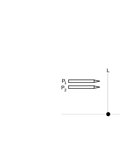
Figure 1. Schematic experimental situation consisting of the two electrical probes $P_{1}$ and $P_{2}$ which can act by electrostatic forces on the cantilever $L$.

Under the initial condition of the cantilever $L$ in the vertical position we can have the following two experimental transitions of the physical system “Probes+Cantilever”:

1. If no electrode voltage $V$ is applied to the two probes, the cantilever remains in the vertical position.

2. If on the contrary an electrode voltage $V\neq 0$ is applied to at least one probe, the position of the cantilever is changed as consequence of the electrostatic force.

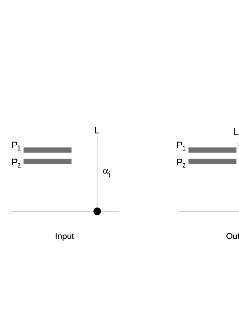
Figure 2. Schematic description of the experimental LNG-device where at least one of the probes ($P_{1}$, $P_{2}$) is active and the initial cantilever position is vertical ($\alpha_{i}=0$). Both probes do not change their state and the cantilever $L$ undergoes a deflection of an output angle $\alpha_{o}\neq 0$.

Let us stress the following interpretation assumed by the authors of [LSNG16] which is the main argument of our analysis:

1. The input of the logic gate is associated with the voltages $V(P_{1})$ and $V(P_{2})$ of the respective electrical probes $P_{1}$ and $P_{2}$. The position of the cantilever tip, measured by its deviation angle $\alpha_{o}$ with respect to the vertical position, encodes the output of the logic gate. In a first approximation, this corresponds to a 2in/1out gate $G_{LNG}$ formalized by the correspondence:

   $$(V(P_{1}),V(P_{2}))\xrightarrow{G_{LNG}}\alpha_{o}$$

   But in the quoted paper it is assumed a drastic convention of associating with the voltages $V(P_{i})$ of the probe $P_{i}$ their “normalized” value $[V(P_{i})]=1$ iff $V(P_{i})\neq 0$ and $[V(P_{i})]=0$ otherwise, i.e., iff $V(P_{i})=0$, corresponding to the logic truth value 1 if the probe is on ($V(P_{i})\neq 0$) and the truth value 0 if the probe is off ($V(P_{i})=0$).
   Similarly for the deviation angle we put $[\alpha]=1$ iff $\alpha\neq 0$, and $[\alpha]=0$ otherwise. With these conventions the authors consider their device as a 2in/1out Boolean gate $G_{LNG}:\{0,1\}^{2}\to\{0,1\}$ defined by the correspondence

   (1) $$\left([V(P_{1})],[V(P_{2})]\right)\xrightarrow{G_{LNG}}[\alpha_{o}]$$

As consequence of all these conventions, i.e., interpreting absence or presence of electric voltage on the probes as logic values 0 and 1, respectively, this device realizes the Or logic gate according to the following table which collects all the above remarks:

$[V(P_{1})]$	$[V(P_{2})]$	$\xrightarrow{LNG}$	$[\alpha_{o}]$
$0$	$0$		$0$
$0$	$1$		$1$
$1$	$0$		$1$
$1$	$1$		$1$

Table 1. Normalized table of the LNG behavior under LNG assumptions

Our position about the LNG realization of the Or gate can be exposed in the following considerations:

1. In the transition depicted by Fig. 2 the input state is applied to the physical system “Probes+Cantilever”, but in order to describe the output state one must take into account that the device continue to be the whole physical system “Probes+Cantilever”.
   Therefore, in line of principle, there is no contra-indication to set the initial position of the cantilever in any possible angle $\alpha_{i}$, of course considering also the particular case $\alpha_{i}=0$, the input configuration must take into account not only the Boolean pair $[V(P_{1})],[V(P_{2})]$, but also the Boolean value $[\alpha_{i}]$.
   But, since during the transformation the physical device continues to be “Probes+Cantilever”, in order to detect the generated output without erasing information about the potentials $V(P_{1})$ and $V(P_{2})$, which produce the output angle of the cantilever $\alpha_{o}$, the real output of the device is the configuration $[V(P_{1})],[V(P_{2})],[\alpha_{o}]$.
   This leads to the following table describing the physical transition different from the previous one relative to the input cantilever angle $\alpha_{i}=0$:

   $[V(P_{1})]$	$[V(P_{2})]$	$[\alpha_{i}]$	$\xrightarrow{CL}$	$[V(P_{1})]$	$[V(P_{2})]$	$[\alpha_{o}]$
   $0$	$0$	$0$		$0$	$0$	$0$
   $0$	$1$	$0$		$0$	$1$	$1$
   $1$	$0$	$0$		$1$	$0$	$1$
   $1$	$1$	$0$		$1$	$1$	$1$

   Table 2. Normalized table of the LNG behavior under CL assumptions

Of course, this corresponds to a partial reversible non conservative 3in/3out gate, whose complete formulation will be the argument of the forthcoming sections. According to this point of view there is no contradiction with the above discussed Landauer principle: the gate is reversible and so we can expected that according to “the experimental results presented in Fig. 3(a) of [LSNG16] the dissipated heat can be reduced below $k_{B}T$.” As usual in reversible logic, the value $[\alpha_{i}]$ set to 0 corresponds to the ancilla input and the output values $[V(P_{1})],[V(P_{2})]$ are the garbage of the logic Or realization by the output $[\alpha_{o}]$. Situations of this kind, making use of the Toffoli’s box representation introduced in [Tof80], can be depicted as the Figure 3.

Figure 3. Toffoli’s box representation of the Or realization according to the CL position. Note that the official Toffoli’s terminology is the following: input=argument, output=result, ancilla=source, garbage=sink

2.1. A formal analysis of the LNG device behavior and an interesting metatheoretical contraposition

In order to better understand the above (LNG) and (CL) two different points of view about the LNG experimental results, let us introduce a formalization of its behavior. First of all let us denote by ${\mathcal{V}}$ the collection of possible voltages applied to the two probes $P_{1}$ and $P_{2}$, and by ${\mathcal{A}}$ the collection of all possible angles assumed by the cantilever with respect to the vertical axis. From a more general point of view we can formalize the functioning of the physical device “Probes+Cantilever” by a function

$$F:{\mathcal{V}}\times{\mathcal{V}}\times{\mathcal{A}}\to{\mathcal{V}}\times{\mathcal{V}}\times{\mathcal{A}}$$

assigning to the input $(V_{1},V_{2},\alpha_{i})$ consisting of the voltage $V_{1}$ (resp., $V_{2}$) applied to the probe $P_{1}$ (resp., $P_{2}$) and the initial angle of the cantilever $\alpha_{i}$ the output

$$F(V_{1},V_{2},\alpha_{i})=(F_{1}(V_{1},V_{2},\alpha_{i}),F_{2}(V_{1},V_{2},\alpha_{i}),F_{3}(V_{1},V_{2},\alpha_{i}))$$

where, as it happens in any multivalued function, the three component functions are put in clear evidence. Precisely, in order to describe the behavior of the LNG device synthesized by the previous points (Ex1)–(Ex2), the component functions $F_{1}:{\mathcal{V}}\times{\mathcal{V}}\times{\mathcal{A}}\to{\mathcal{V}}$, $F_{2}:{\mathcal{V}}\times{\mathcal{V}}\times{\mathcal{A}}\to{\mathcal{V}}$, and $F_{3}:{\mathcal{V}}\times{\mathcal{V}}\times{\mathcal{A}}\to{\mathcal{A}}$ are defined by the laws

$$F_{1}(V_{1},V_{2},\alpha_{i})=V_{1},\;F_{2}(V_{1},V_{2},\alpha_{i})=V_{2},\;\text{and}\;F_{3}(V_{1},V_{2},\alpha_{i})=\alpha_{o}$$

In the particular case depicted in Fig. 2 in which the initial angle is $\alpha_{i}=0$ we have

$$F_{1}(V_{1},V_{2},0)=V_{1}$$

$$F_{2}(V_{1},V_{2},0)=V_{2}$$

$$F_{3}(V_{1},V_{2},0)=\alpha_{o}$$

Now with respect to this formalization there are at least two possible descriptions:

1. According to (LNG) in considering the output results one can neglect what happens in the two probes, that is one disregards the two component functions $F_{1}$ and $F_{2}$, considered as hidden, and so in describing the experiment one takes into account the sole function $F_{3}(V_{1},V_{2},\alpha_{i})=\alpha_{o}$ in which the output $\alpha_{0}$ uniquely depends from $V_{1}$ and $V_{2}$ producing the gate of Table 1 for realizing the Or connective in an irreversible way.

2. According to (CL) also in describing the output results one must take into account the whole ${\mathcal{V}}\times{\mathcal{V}}\times{\mathcal{A}}$ situation of the experimental apparatus “Probes+Cantilever”, that is the whole three component functions $F_{1},F_{2}$, besides to $F_{3}$, leading to the gate described by Table 2 for realizing the Or connective in a reversible way.

Relatively to the above discussion we have

• the theoretical Landauer principle whose validation or falsification can be obtained by experiments;

• the LNG experimental device which realizes the connective Or with an arbitrary small dissipation of energy.

So, there are two possible contradictory positions:

1. If a priori one is against the Landauer principle, then one accepts the above position (Po1) claiming that the experimental LNG results falsify the Landauer principle.

2. If a priori one accepts the Landauer principle, then one agrees with the above description (Po2) of the experimental LNG results as a corroboration of the Landauer principle.

A very interesting situation for an epistemological/philosophical debate where the experimental results, according to one or the opposite other assumption, lead to a falsification or a corroboration of the same theoretic principle.

We of course support the position (Po2). It is out of any doubt that the experimental LNG device is formed by the physical system “Probes ($P_{1},P_{2}$)+Cantilever ($L$)” and so a formal description of its input state must consist of a triple $(V_{1},V_{2},\alpha_{i})$ formed by the two input probe voltages $V_{1}$ and $V_{2}$ and the input initial angle $\alpha_{i}$ (left side of Figure 2). After the interaction the physical LNG device continue to consist of the pair “Probes ($P_{1},P_{2}$)+Cantilever ($L$)” and so in order to describe this physical situation the output state must be formed by the complete information about not only the output angle $\alpha_{o}$, but also of the probe voltages (right side of Figure 2), producing the reversible transition described by the Table 2. In other words, also in the output case we must have a complete description of the physical state of the “Probes+Cantilever” device.

On the contrary, as supported by LNG, if one decides that in the case of the output the physical system collapses in the cantilever component disregarding what happens to the two probes, then the output state consists in the unique variable “output angle” $\alpha_{o}$, i.e., a hidden variables incomplete description, corresponding to the irreversible transition described in Table 1.

Comparing these two positions, we can say that our description is a reversible completion of the incomplete (with hidden variables) irreversible LNG description. This is the reason which leads us to adopt the reversible completion version of the hidden incomplete irreversible one as interesting argument of investigation in the forthcoming sections. In particular, in the next subsection we confirm the rightness of this choice just on the basis of some experimental results obtained by the LNG device.

2.2. A first reversible version of the LNG device

Coming back to the LNG device described at the beginning of section 2 and depicted in Figg. 1 and 2, owing to the fact that the input voltages $V(P_{1})=0$ and $V(P_{2})=0$ produce the trivial output $\alpha_{o}=0$, the main interesting results regard the measure of the angle deviation of the cantilever $\alpha_{o}$ in the three cases of input interest $[V(P_{1})][V(P_{2})]=01,10,11$. Since the cantilever is really very small, the position change of its tip, as consequence of the bent, is also very small and subjected to thermal fluctuations. Hence, the statistical distribution of the cantilever tip position is a random quantity well reproduced by a Gaussian curve. It is experimentally observed (see Fig. 2(b) from [LSNG16, pag. 2]) that

• logic inputs corresponding to the states $01$ e $10$ produce very similar results, distributed in a range between 0.8 nm and 1 nm,

• whereas the logic input 11 produces a larger displacement around 1.1 nm.

Of course, if one agrees with these considerations then one can achieve the following LNG conclusions:

1. if the similarity of the results obtained by the inputs 01 and 10 is assumed as an element of their indistinguishability, considering them as the production of the same output 1, and also if the larger displacement produced by the input 11 is always associated to the same output 1, one can conclude that “the cantilever-based gate performs like an Or gate that is a logical irreversible device [see Table 1]: in fact there is at least one case [i.e., 01, 10, 11] where, from the sole knowledge of the logic (and physical) output [i.e., 1], it is not possible to infer the status of the logic inputs.” [LSNG16].

This is a possible metatheoretical position which can be considered as a joke of a dark night in which all the cows [inputs 01, 10, 11] result of colour black [the same output 1]. On the basis of the obtained results, our position is on the contrary quite different and in agreement with the previous considerations collected in the above statement (CL). Precisely, referring to the experimental results of Fig. 3(a) of [LSNG16], for any fixed protocol time $\tau_{p}$ (ms) the average produced heat gives three different results always interpreted as the output 1 but relatively to the inputs 10 (symbol $\circ$), 01 (symbol $\vartriangle$), and 11 (symbol $\square$).

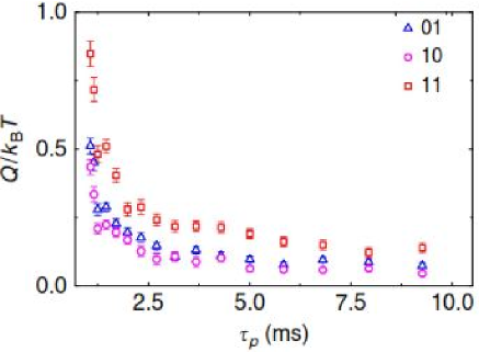
Figure 4. Experimental results of Figure 3(a) from [LSNG16, pag. 4]

Once adopted the convention of identifying the following symbols

(2) $$10\equiv\circ\qquad 01\equiv\vartriangle\qquad 11\equiv\square$$

it is really true that the experimental outputs produced by 10 and 01 are very near, as said before “very similar”, between them, but as evident from the above Figure 4, reproduction of the original Figure 3(a) from [LSNG16],

the $\circ$ are always less in value with respect to $\vartriangle$, and furthermore the output $\square$ furnishes always a value resolutely greater that these two.

This behavior is confirmed by the histograms of Fig. 2(c) of [LSNG16, pag. 2] in which the one corresponding to the input 10 ($\circ$) assumes the maximum value lightly near to the value 0.8 nm, whereas the one corresponding to the input 01 ($\vartriangle$) shows the maximum value lightly near to the value 1.0 nm, in any case greater that the previous one. Lastly, the histogram of the input 11 ($\square$) has a maximum between 1.0 and 1.2 nm, but near this latter value and in any case clearly distinguishable from the other two.

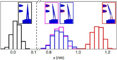
Figure 5. Histograms of Figure 2(c) from [LSNG16, pag. 2]

In this paper we assume that they correspond to three “different” values of the logic value 1 according to the following statement:

1. Borrowing the usual terminology from the fuzzy set theory according to Zadeh we can think to three different logic values 1, each of them characterized by the “membership degree” represented by the three symbols $\circ$, $\vartriangle$, and $\square$, formalized as ordered pairs $(\circ,1)$, $(\vartriangle,1)$, e $(\square,1)$.

Then, according to this interpretation, the LNG gate for realizing the logic connective Or is formalized by the transitions:

(3)

LNG–Or

Input Output

$$00$$

where for formal completeness we used the symbol $*$ associated to the logic value 0 in order to obtain the output $(*,0)$, omitting its precise determination which will be made in the sequel. In this way we obtain a reversible gate since the knowledge of any output allows one to uniquely determine the corresponding input generating it. In this way we lose any possible ambiguity, and with respect to this result we can do the following remark.

It is very interesting to note that these pure experimental results are completely described in a right way by (i.e., it is totally coincident with) our Table 2 once adopted in this latter the above conventional substitutions given by equation (2). In this way the experimental results of Fig. 2(b) from [LSNG16]) confirm the rightness of our previous assumptions formalized in (Po2) relative to a 3in/3out reversible gate description of the LNG experiment, and so without any contradiction with respect to the experimental result of arbitrary small dispersion of energy, according to the Landauer principle.

At any rate we don’t continue to develop this interesting analysis since in the next section we formalize a realization of the LNG device as a 3in/3out self–reversible gate, avoiding any discussion about the dichotomy “01 and 10 distinguishable or indistinguishable”, but which satisfies the Landauer principle owing to its reversibility.

3. The self–reversible 3in/3out Cattaneo Leporini (CL) gate

In order to obtain this result first of all we have analyzed the main 3in/3out gates which one can found in literature: the conservative self–reversible Fredkin gate, the self–reversible but not conservative Toffoli and Peres gates (see [FT82, Per85]) realizing that no of them satisfies the condition of having as derived gate, that is fixing one of the input as ancilla and considering two of the outputs as garbage, the description of the LNG device. As a consequence we have autonomously construct a gate of this kind arriving to the Cattaneo–Leporini (CL) 3in/3out gate $G_{\text{CL}}$ described by the following functional representation (but discovering some times after our formalization that the same gate has been introduced in [KTR12] with the name of TNor gate).

(4) $$\text{CL Gate}=\begin{cases}x^{\prime}_{1}=x_{1}\\ x^{\prime}_{2}=x_{2}\\ x^{\prime}_{3}=(x_{1}\lor x_{2})\oplus x_{3}\end{cases}$$

This functional definition is represented by the Table 3.

$x_{1}$	$x_{2}$	$x_{3}$	$\xrightarrow{G_{CL}}$	$x^{\prime}_{1}$	$x^{\prime}_{2}$	$x^{\prime}_{3}$
$0$	$0$	$0$		$0$	$0$	$0$
$0$	$0$	$1$		$0$	$0$	$1$
$0$	$1$	$0$		$0$	$1$	$1$
$0$	$1$	$1$		$0$	$1$	$0$
$1$	$0$	$0$		$1$	$0$	$1$
$1$	$0$	$1$		$1$	$0$	$0$
$1$	$1$	$0$		$1$	$1$	$1$
$1$	$1$	$1$		$1$	$1$	$0$

Table 3. Tabular representation of the 3in/3out self-reversible CL gate

Obviously, this is a reversible non–conservative gate (for instance, in the transition $(010)\to(011)$ the number of 1 bites in the input is not preserved). Moreover, it is self–reversible in the sense that

(5) $$G_{\text{CL}}\circ G_{\text{CL}}=\text{id}$$

That is, the inverse of $G_{\text{CL}}$ is the $G_{\text{CL}}$ itself: $G_{\text{CL}}^{-1}=G_{\text{CL}}$. Below in Fig. 6 it is represented the role played by self–reversibility in producing as global output the same input as consequence of the transitions $(a,b,c)\xrightarrow{CL}(a,b,(a\lor b)\oplus c)\xrightarrow{CL}(a,b,c)$. The FanOut (FO) reversible, but non conservative, gate allows the duplication (cloning) of the signal of the third line after the first output, a duplication of which is inserted as third input of the second CL gate, whereas the other duplication is extracted as overall output of the cascade.

Figure 6. Self–reversibility of the CL gate, with the FO gate for the cloning of the third line of the first output

From the functioning of the CL gate described in the Table 3 it follows that, if as usual some suitable inputs are fixed as ancilla, one has the following possible cases:

$$(0,a,b) \to(0,a,a\oplus b) (a,0,b) \to(a,0,a\oplus b) (a,b,0) \to(a,b,a\lor b)$$

$$(1,a,b) \to(1,a,\neg b) (a,1,b) \to(a,1,\neg b) (a,b,1) \to(a,b,\neg(a\lor b))$$

corresponding to the realization of the logic connectives Xor $\oplus$, Or $\lor$, and Nor $\neg\lor$. Moreover, below one can find some realizations of the FanOut gate:

$$(a,0,0)\to(a,0,a)\qquad(0,a,0)\to(0,a,a)$$

There are also some different possibilities of realizing the logic connective Not $\neg$, of which below we show some of them:

(6a) $$(0,1,b)\to(0,1,\neg b)\qquad(1,0,b)\to(1,0,\neg b)\qquad(1,1,b)\to(1,1,\neg b)$$

(6b) $$(a,0,1)\to(a,0,\neg a)\qquad(0,b,1)\to(0,b,\neg b)$$

Summarizing, the primitive logic connectives which can be obtained from this 3in/3out self–reversible CL gate can be collected in the following list:

$$\mathcal{G}_{C}=\{\textsc{Xor},\textsc{Or},\textsc{Nor},\textsc{Not},\textsc{Fan}\textsc{Out}\}$$

Let us note a behavior of this CL gate which in some sense is dual with respect to the Toffoli gate, as successively discussed by a comparison of it with this latter, and of which we will study the analogies in the forthcoming section. This behavior consists in the transitions:

(7) $$(0,0,c)\xrightarrow{a\land b=0}(0,0,c)\qquad(a,b,c)\xrightarrow{a\lor b=1}(a,b,\neg c)$$

in which we stress that if the first and the second lines are both fixed in the input 0 ($a\land b=0$) then on the third line it acts the identity, whereas in all the other cases in which at least one of the two control lines, the first and the second ones, is fixed with the input 1 ($a\lor b=1$) then on the third line it is the Not gate which acts. It is a kind of Controlled–Controlled–(multiple)Not (CCmN) in which $a$ and $b$ are known as the first and second control bits, while $c$ is the target bit. In conclusion, the gate leaves both control bits unchanged, flips the target bit if at least one of the control bit is set to 1, and otherwise leaves the target bit alone. We speak of multipleNot since we have seen in the second transition of the equation (7) how it is possible to generate in three different modes the Not logic gate when at least one of the inputs $a$ or $b$ is fixed in the bit 1 (see also the equations (6a)).

Let us now analyze the behavior of our self–reversible CL gate when the third input is fixed to $x_{3}=0$, which turns out to be useful in the sequel for a comparison with the LNG realization of their Or gate. We extract this behavior from the Table 3 when the third input is set to 0, obtaining the partial Table 4 (which is identical to the Table 2 under the identifications $x_{1}=x^{\prime}_{1}=[V(P_{1})]$, $x_{2}=x^{\prime}_{2}=[V(P_{2})]$, and $x_{3}=[\alpha_{i}]$, $x^{\prime}_{3}=[\alpha_{o}]$):

$x_{1}$	$x_{2}$	$x_{3}$	$\xrightarrow{G_{CL}}$	$x^{\prime}_{1}$	$x^{\prime}_{2}$	$x^{\prime}_{3}$
$0$	$0$	$0$		$0$	$0$	$0$
$0$	$1$	$0$		$0$	$1$	$1$
$1$	$0$	$0$		$1$	$0$	$1$
$1$	$1$	$0$		$1$	$1$	$1$

Table 4. Realization of the Or connective by the output $x^{\prime}_{3}=x_{1}\lor x_{2}$ from the CL self-reversible 3in/3out gate fixing the input $x_{3}=0$

This situation produces the self–reversible transitions:

$$(a,b,0)\to(a,b,a\lor b)\to(a,b,0)$$

represented in the block scheme of Figure 7.

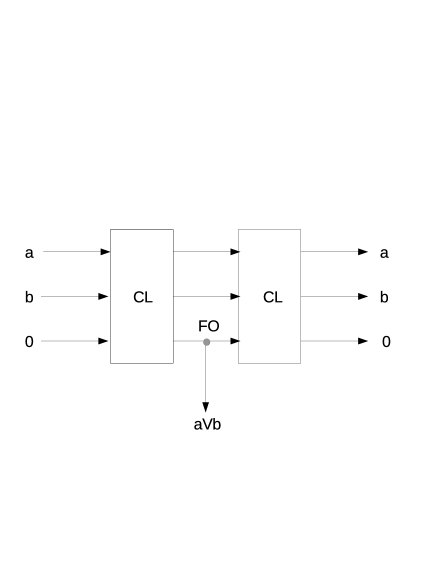
Figure 7. Self–reversibility of the CL gate for $x_{3}=0$, with the FO gate for the cloning of the third output of the first gate generating the Or logic connective

Note that if on the contrary in the CL gate of Table 3 the third input is fixed to 1, $x_{3}=1$, then both the first and the second line produce the identity whereas the third output furnishes the self-reversible Nor gate realization according to the transitions:

$$(a,b,1)\to(a,b,\neg(a\lor b))\to(a,b,1)$$

depicted in the Figure 8.

Figure 8. Self–reversibility of the CL gate for $x_{3}=1$, with the FO gate for the cloning of the third output of the first gate generating the Nor logic connective

Let us finish this section with the analysis of another possible behavior of the CL gate. Precisely the one in which the first line has an output which remains unchanged $x^{\prime}_{1}=x_{1}$, but with the two input bits 0 and 1 which produce two different situations acting as different gates on the remaining two lines $x_{2}-x^{\prime}_{2}$ e $x_{3}-x^{\prime}_{3}$ according to the following tables.

(8)

fixed line 0 id 0

first line a id a

second line b $$\oplus$$

      

fixed line 1 id 1

first line a id a

second line b

4. The self–reversible 3in/3out Toffoli (T) gate

In literature one can find an interesting reversible, non conservative, gate introduced by Toffoli by the functional representation:

(9) $$\text{Toffoli Gate}=\begin{cases}x^{\prime}_{1}=x_{1}\\ x^{\prime}_{2}=x_{2}\\ x^{\prime}_{3}=(x_{1}\land x_{2})\oplus x_{3}\end{cases}$$

whose comparison with the functional representation of the CL gate of equation (4) stressed the difference consisting in substituting into the third equation of this latter the connective $\lor$ with the connective $\land$. The Toffoli gate formulation in terms of truth table is the following one:

$x_{1}$	$x_{2}$	$x_{3}$	$\xrightarrow{G_{T}}$	$x^{\prime}_{1}$	$x^{\prime}_{2}$	$x^{\prime}_{3}$
$0$	$0$	$0$		$0$	$0$	$0$
$0$	$0$	$1$		$0$	$0$	$1$
$0$	$1$	$0$		$0$	$1$	$0$
$0$	$1$	$1$		$0$	$1$	$1$
$1$	$0$	$0$		$1$	$0$	$0$
$1$	$0$	$1$		$1$	$0$	$1$
$1$	$1$	$0$		$1$	$1$	$1$
$1$	$1$	$1$		$1$	$1$	$0$

Table 5. Tabular representation of the 3in/3out self-reversible Toffoli gate

From which, by constraining one of the inputs as ancilla, it is possible to obtain some familiar standard logic primitives, according to the correspondences

$$(0,a,b) \to(0,a,b) (a,0,b) \to(a,0,b) (a,b,0) \to(a,b,a\land b)$$

$$(1,a,b) \to(1,a,(a\oplus b)) (a,1,b) \to(a,1,a\oplus b) (a,b,1) \to(a,b,\neg(a\land b))$$

whereas, by constraining two of the inputs, we may get the FanOut and the Not gates, for instance

$$(a,1,0)\to(a,1,a)\qquad(1,b,0)\to(1,b,b)\qquad(a,1,1)\to(a,1,\neg a)\qquad(1,b,1)\to(1,b,\neg b)$$

Summarizing the set of logic primitives generated by the self–reversible Toffoli gate is the following one:

$$\mathcal{G}_{T}=\left\{\textsc{Xor},\textsc{And},\textsc{Nand},\textsc{Not},\textsc{Fan}\textsc{Out}\right\}$$

Let us recall that this Toffoli gate is the one that Feynman in [Fey96] defines (and presently is recognized as such) Controlled Controlled Not (CCN): “in which the lines $x_{1}$ and $x_{2}$ acts as control lines, leaving $x_{3}$ as it is unless both are one, in which case $x_{3}$ becomes Not($x_{3}$).” This behavior can be described by the correspondences, which can be compared with the analogous of the CL gate expressed by equation (7),

(10) $$(a,b,c)\xrightarrow{a\lor b=0}(a,b,c)\qquad(1,1,c)\xrightarrow{a\land b=1}(1,1,\neg c)$$

Similarly to the CL gate, fixing the input $x_{3}=0$ as ancilla, the Toffoli gate reduces to the following table producing the output $x^{\prime}_{3}=x_{1}\land x_{2}$ with the pair $x^{\prime}_{1},x^{\prime}_{2}$ as garbage, i.e., a reversible realization of the And logic connective.

$x_{1}$	$x_{2}$	$x_{3}$	$\xrightarrow{G_{T}}$	$x^{\prime}_{1}$	$x^{\prime}_{2}$	$x^{\prime}_{3}$
$0$	$0$	$0$		$0$	$0$	$0$
$0$	$1$	$0$		$0$	$1$	$0$
$1$	$0$	$0$		$1$	$0$	$0$
$1$	$1$	$0$		$1$	$1$	$1$

Table 6. Realization of the And connective by the output $x^{\prime}_{3}=x_{1}\land x_{2}$ from the Toffoli self-reversible 3in/3out gate fixing the input $x_{3}=0$

This situation of the Toffoli gate produces the self-reversible transitions:

$$(a,b,0)\to(a,b,a\land b)\to(a,b,0)$$

The logic connective Nand, $\neg(a\land b)$, is obtained by the Toffoli gate if we input $x_{1}=a$ and $x_{2}=b$ as control bits, and fixing as ancilla bit the third input $x_{3}=1$. The Nand of $x_{1}$ and $x_{2}$ is output as the target $x^{\prime}_{3}$ considering the pair formed by the first and the second outputs $(x^{\prime}_{1}=a,x^{\prime}_{2}=b)$ as garbage. Formally, this can be formalized by the transitions, where the second one stresses the self-reversibility of the gate:

$$(a,b,1)\to(a,b,\neg(a\land b))\to(a,b,1)$$

Quoting Peres “It is well known that the Nand gate is a universal primitive (Nand is the relational operator which gives the ”true” value as output if one or both input values are ”false.”) Therefore the reversible gate [of Table 5] is universal.”

5. LNG Or and And connectives implementation by self-reversible gates

Let us first consider the Or gate realization using the device proposed by López-Suárez et al. in [LSNG16] (schematically depicted in Fig. 1 of our section 2). As previously described the device consists of two electrical probes (denoted by $P_{1}$, $P_{2}$) close to a cantilever $L$. An electrode voltage $V$ can be applied to each probe $P_{j}$. If $V=0$, we will say the probe is off (denoted by $D$), while we will say the probe is on (denoted by $A$) when $V\neq 0$. The corresponding cantilever tip displacement is determined by the angle $\alpha$ formed with respect to the vertical axis as reference axis.

The experimental results obtained by the LNC device represented by Fig. 2(c) from [LSNG16] can be summarized in the following points:

1. Under the fixed input initial angle $\alpha_{i}=0$ of the cantilever, a sufficiently large number of single tests, each of which relative to the three non “trivial” inputs of the voltages applied to the two probes $DA$, $AD$, and $AA$, experimentally produces three histograms $I_{DA}$, $I_{AD}$, and $I_{AA}$ as mappings $\alpha\in{\mathbb{R}}_{+}\to I_{hk}(\alpha)\in{\mathbb{N}}$, for $hk$ ranging on $\{DA,AD,AA\}$.

2. Each histogram has a support (collection of $\alpha\in{\mathbb{R}}_{+}$ for which the corresponding $I_{hk}(\alpha)\neq 0$), denoted as $supp(I_{hk})$, which is a bounded interval on ${\mathbb{R}}_{+}$.

3. There is a bounded value of angle $\alpha_{B}$, such that both the supports $I_{DA}<\alpha_{B}$ and $I_{AD}<\alpha_{B}$, whereas $\alpha_{B}<I_{AA}$.

4. The two supports $I_{DA}$ and $I_{AD}$ are quite similar, $I_{DA}\simeq I_{AD}$, and so according to the LNG assumption described in the point (LNG-1) of section 2.2, they can be submitted to the stronger condition of being equal: $I_{DA}=I_{AD}$.

5. All the above histograms $I_{hk}$ correspond to statistical distributions well reproduced by Gaussian curve. Denoted by $\hat{\alpha}_{1}=<I_{DA}>$, $\tilde{\alpha}_{1}=<I_{AD}>$, and $\alpha_{2}=<I_{AA}>$, the corresponding mean value of the involved Gaussian, ad as usual in physics putting the boundary angle $\alpha_{B}=1$, the experimental results give the following chain of values:
   $0<\hat{\alpha}_{1}\simeq\tilde{\alpha}_{1}<1<\alpha_{2}$.

6. According to the strong assumption of point (Exp4), this last result can be formalized by the chain of inequalities:

   (11) $$0<\hat{\alpha}_{1}=\tilde{\alpha}_{1}<1<\alpha_{2}$$

We recall that all these experimental results follow by the initial condition on the input angle $\alpha_{i}=0$, and so all these results can be collected in the following table where, according to the strong assumption (Exp6) formalized in the chain of inequalities (11), we set $\alpha_{1}:=\hat{\alpha}_{1}=\tilde{\alpha}_{1}$.

$P_{1}$	$P_{2}$	$\alpha_{i}$	$\longmapsto$	$P^{\prime}_{1}$	$P^{\prime}_{2}$	$\alpha_{o}$
$D$	$D$	$0$		$D$	$D$	$0$
$D$	$A$	$0$		$D$	$A$	$\alpha_{1}$
$A$	$D$	$0$		$A$	$D$	$\alpha_{1}$
$A$	$A$	$0$		$A$	$A$	$\alpha_{2}$

Table 7. Physical behavior of the LNG device when the cantilever is in the initial vertical position $\alpha_{i}=0$ and the ordering of the final angles $\alpha_{o}$ given by $0<\alpha_{1}<1<\alpha_{2}$

Assuming now the convention of putting $A=1$ (probe on, i.e., active) and $D=0$ (probe off, i.e., inactive) these results can be translated in a Boolean context under particular assumptions about a normalization function of the angle $\alpha$ according to two possible cases which we will discuss now.

5.1. First normalization function: the Cattaneo-Leporini case for generating Or

In this first case the normalization function of the angle, denoted by $u_{1}(\alpha)$, is the following one:

$$u_{1}(\alpha)=\begin{cases}0&\text{if}\;\alpha=0\\ 1&\text{otherwise}\end{cases}$$

From this choice of normalization function, the physical behavior of the LNG device described in the Table 7 when the initial cantilever position is vertical, $\alpha_{i}=0$, is translated into the table of equation (12) at the left side. The Boolean table at the right is nothing else than this latter setting $A=1$, $D=0$, $P_{1}=x_{1}$, $P_{2}=x_{2}$, $u_{1}(\alpha_{i})=x_{3}$, and $u_{1}(\alpha_{o})=x^{\prime}_{3}$:

(12)

$$P_{1}$$

      

But, looking at these experimental results from the LNG device we con set the following interesting considerations:

• The table at the right giving the Boolean formalization of the LNG device behavior when the initial cantilever angle is 0 coincides with the Table 4 discussed in section 3 as self-reversible CL gate realization of the classical Or connective under the ancilla choice $x_{3}=0$, the third output $x^{\prime}_{3}=x_{1}\lor x_{2}$ producing the required Or, and with the two outputs $x^{\prime}_{1}$ and $x^{\prime}_{2}$ as garbage (see also the description given by Fig. 3 and 7).

• That is, all the experimental results obtained by the LNG concrete device and collected in the above Table 7 can be described by a 3in/3out self-reversible Boolean gate with a complete agreement with the Landauer principle of arbitrary small energy dissipation.

• In other words, there is no experimental contradiction as claimed by LNG in their paper.

Furthermore, encoding the output $(x^{\prime}_{1},x^{\prime}_{2})$ as follows $00=*,\,01=\vartriangle,\,10=\circ,\,11=\square$, the table (12) at the right side becomes the following (that can be compared with Table (3), according to our point of view about the experimental results obtained from the LNG device described in section 2.2):

(13)

$$x_{1}x_{2}$$

Therefore, if in the left table (12) we consider the case where at least one of the probes is active, we will have the following three transitions:

$$(DA,u_{1}(\alpha_{i})=0)\xrightarrow{LNG}(DA,u_{1}(\alpha_{o})=1)$$

$$(AD,u_{1}(\alpha_{i})=0)\xrightarrow{LNG}(AD,u_{1}(\alpha_{o})=1)$$

$$(AA,u_{1}(\alpha_{i})=0)\xrightarrow{LNG}(AA,u_{1}(\alpha_{o})=1)$$

In these cases, when the result of the interaction of the probes $P_{1},P_{2}$ on the cantilever $L$ is observed, one cannot overlook/disregard the two probes to only look at the tip position, but one has to consider the whole apparatus “probes + cantilever tip” (see Fig. 2).

Following the right table (12), we have the whole transitions:

$$(01|0)\xrightarrow[CL]{LNG}(01|1)=(\vartriangle|1)$$

$$(10|0)\xrightarrow[CL]{LNG}(10|1)=(\circ|1)$$

$$(11|0)\xrightarrow[CL]{LNG}(11|1)=(\square|1)$$

where the output in $\{0,1\}^{3}$ (whether it is $(01|1)$ or $(10|1)$ or $(11|1)$) uniquely determines the input in $\{0,1\}^{3}$ generating it, and so, stressing this conclusion another time, according to the Landauer principle without any dissipation of energy. All this has nothing to do with the 2in/1out irreversible Or logic gate where the output $1$ does not allow one to determine the generating input in $\{0,1\}^{2}$, as claimed by LNG in their paper.

As a summary of all the above discussion we can state the

1st Conclusion:

The LNG device under the assumptions of the initial cantilever angle $\alpha_{i}=0$ and the normalized function on angles $u_{1}$ is a concrete realization of the CL 3in/3out self-reversible gate with the third input fixed to 0, producing in the third output the connective Or.

5.2. Second normalization function: the Toffoli case for generating And

As said before, the Boolean formulation of the experimental results collected in Table 7 depends from an arbitrary choice of a normalization function assigning in a conventional way Boolean values to the cantilever angles. In the present subsection we take into account another possible conventional choice formalized by the normalization function:

$$u_{2}(\alpha)=\begin{cases}0&\text{if}\;0\leq\alpha\leq 1\\ 1&\text{otherwise}\end{cases}$$

In this case the Table 7, with the usual adopted conventions, leads to the following two tables

(14)

$$P_{1}$$

      

The table at the right coincides with the Table 5 obtained from the self-reversible 3in/3out Toffoli gate fixing the input ancilla $x_{3}=0$, with the pair $x^{\prime}_{1}x^{\prime}_{2}$ considered as garbage, and the output $x^{\prime}_{3}=x_{1}\land x_{2}$ furnishing the logic And of the first and second inputs. So also in this case we have a “reversible” generation of the required And gate with arbitrary small dissipation of energy. This result involving the self-reversible Toffoli gate has been achieved adopting a normalization function for describing the experimental results produced by the LNG device different from the one adopted in the CL case. But let us stress that these two different choices correspond to some quite arbitrary Boolean assignments to the involved cantilever angles, no one of which can be considered as a privileged choice from the experimental point of view.

This behavior has been also realized by LNC when in the discussion about the Fig. 2(c) they assert that “the threshold value for the Or gate is represented by the dashed line [around 0.1 nm]. By changing the position of the dashed line [around 1.0 nm], the gate can be operated also as an And gate.” Precisely, the dashed line around 0.1 nm put the three situations 01, 10, and 11 as associated to the output state 1, whereas the dashed line around 1.0 nm groups the three situations 00, 01, and 10 as associated to the output state 0.

As a summary of the discussion performed in this subsection we can state the

2nd Conclusion:

The LNG device under the assumptions of the initial cantilever angle $\alpha_{i}=0$ and the normalized function on angles $u_{2}$ is a concrete realization of the Toffoli 3in/3out self-reversible gate with the third input fixed to 0, producing in the third output the connective And.

6. Nor and Nand connectives implementations by LNG device

Let us recall that, as stressed before, the assignment of a Boolean bit value, either 0 or 1, to a deflection angle formed by the cantilever is only a conventional matter of fact. There is no physical reason to state that, for instance, a particular angle $\alpha$ may be labelled with the bit value 1 instead of the bit value 0. This is the reason that allowed us to consider two different normalization functions, $u_{1}$ and $u_{2}$, to treat the above cases of subsections 5.1 and 5.2, respectively, in order to prove that the LNG device, suitably normalized, describes the Or and the And logic connectives by self-reversible CL and Toffoli gates.

6.1. Third normalization function: the Cattaneo-Leporini case for generating Nor

Let us apply to the functioning of the LNG device described by the Table 7 the conventional normalization function $\overline{u}_{1}:=1-u_{1}$, explicitly written as

$$\overline{u}_{1}(\alpha):=\begin{cases}1&\text{if}\;\alpha=0\\ 0&\text{otherwise}\end{cases}$$

With the usual conventions the Table 7 is translated into the Boolean form:

(15)

$$x_{1}$$

That is, the fixed bit $x_{3}=1$ is the ancilla input, whereas $x^{\prime}_{3}=\neg(x_{1}\lor x_{2})$ is the required Nor connective produced by the LNG device under the new normalization function. But this is just the same situation described by the self-reversible CL gate depicted in Fig. 8 corresponding to the transitions $(a,b,1)\xrightarrow{CL}(a,b,\neg(a\lor b))\xrightarrow{CL}(a,b,1)$ discussed in section 3. Therefore we can state the following

3rd Conclusion:

The LNG device under the assumptions of the initial cantilever angle $\alpha_{i}=0$ and the normalized function on angles $\overline{u}_{1}$ is a concrete realization of the CL 3in/3out self-reversible gate with the third input fixed to 1, producing in the third output the connective Nor.

6.2. Fourth normalization function: the Toffoli case for generating Nand

Analogously to the previous case, one can apply to the LNG device described by the Table 7 the conventional normalization function $\overline{u}_{2}:=1-u_{2}$, explicitly written as

$$\overline{u}_{2}(\alpha):=\begin{cases}1&\text{if}\;0\leq\alpha\leq 1\\ 0&\text{otherwise}\end{cases}$$

In this case, with the usual conventions the Table 7 is translated into the Boolean form:

(16)

$$x_{1}$$

That is, fixing the third input with the bit $x_{3}=1$, the third output $x^{\prime}_{3}=\neg(x_{1}\land x_{2})$ is the required Nand connective produced by the LNG device under the new normalization function. But this is just the same situation described by the self-reversible Toffoli gate corresponding to the transitions $(a,b,1)\xrightarrow{T}(a,b,\neg(a\land b))\xrightarrow{T}(a,b,1)$ discussed at the end of section 4. Therefore we can state the following

4th Conclusion:

The LNG device under the assumptions of the initial cantilever angle $\alpha_{i}=0$ and the normalized function on angles $\overline{u}_{2}$ is a concrete realization of the Toffoli 3in/3out self-reversible gate with the third input fixed to 1, producing in the third output the connective Nand.

7. The particular case of the LNG realization of the connective Xor

In this section we will take into account the self-reversible realization of Xor logic connective by the LNG device, making use as usual of some suitable normalization function. But first of all let us note that if we take into account the CL self-reversible gate of section 3, this connective can be realized either fixing the first input to 0 (and this in the LNG device corresponds to fixing the voltage of the first probe) or fixing the second input to 0 (and also in this case it is the voltage of the second probe in the LNG device which must be fixed). The same considerations can be done in the Toffoli case where the fixed either first or second input must be 1. This gives rise to a problem as we discuss now.

Let us consider the case of the CL gate for the fixed input $x_{1}=0$, which produces as the third output the Xor logic connective of the second and third inputs, $x^{\prime}_{3}=x_{2}\oplus x_{3}$, whose table describing this case is the following:

$x_{1}$	$x_{2}$	$x_{3}$	$\xrightarrow{G_{CL}}$	$x^{\prime}_{1}$	$x^{\prime}_{2}$	$x^{\prime}_{3}$
$0$	$0$	$0$		$0$	$0$	$0$
$0$	$1$	$0$		$0$	$1$	$1$
$0$	$0$	$1$		$0$	$0$	$1$
$0$	$1$	$1$		$0$	$1$	$0$

Table 8. The Xor connective realization by the CL gate as the third output $x^{\prime}_{3}=x_{2}\oplus x_{3}$ for the first line fixed to $x_{1}=x^{\prime}_{1}=0$

But trying to implement the CL gate inputs $x_{1}x_{2}x_{3}$ into the LNG device, applying the usual physical behaviors described by (Exp1)–(Exp6) in section 5 and making use of the normalization function of subsection 5.1 relative to the CL case, one obtains the following two tables (the left physical table and the corresponding Boolean one at the right):

(17)

$$P_{1}$$

      

As immediate comparison, the Boolean LNG $x^{\prime}_{3}$ of the table (17) at the right has nothing to do with $x_{2}\oplus x_{3}$ obtained in the Table 8 describing the CL case. In order to overcome this drawback in the present section we propose two solutions.

7.1. A first solution for the Xor generation by the LNG device

The first solution regards what happens if we consider $x^{\prime}_{3}:=|u_{1}(\alpha_{i})-u_{1}(\alpha_{o})|$ instead of $u_{1}(\alpha_{o})$. Let’s see if this choice has some interest or possible physical realization. We will have two cases, each with its two subcases:

$|u_{1}(\alpha_{i})-u_{1}(\alpha_{o})|=0$:

1. i.e., if the tip is initially vertical, it remains vertical;

2. i.e., if the tip is deflated by $\alpha_{i}\neq 0$, it remains deflected, although the two angles might be different $\alpha_{i}\neq\alpha_{o}$.

$|u_{1}(\alpha_{i})-u_{1}(\alpha_{o})|=1$:

1. i.e., if the tip is initially vertical, after processing it is deflated;

2. i.e., if the tip is deflated by $\alpha_{i}\neq 0$, eventually, it returns to the vertical position.

These are, at least in principle, all physically observable, but one has to change (or rather, complete) the left LNG table (17) as follows:

(18)

$$P_{1}$$

0

1

1

0

where, setting $x^{\prime}_{3}=|u_{1}(\alpha_{i})-u_{1}(\alpha_{o})|$, one obtains the following table where the third output is the Xor of the second and third input, while the first and second lines retain their value unchanged:

$$x_{1}$$

Note that even in this case one has to do with the realization of the self-reversible Xor (each output is generated by a single input) as the third output in a 3in/3out gate.

7.2. Coherence of the CL through LNG with the present approach

The question arises if what is obtained in the section 5.1 is still valid when the left table (12), in which the only results of $u_{1}(\alpha_{0})$ are considered, is completed with a further final column relative to the outputs $|u_{1}(\alpha_{i})-u_{1}(\alpha_{o})|$. This leas to the following table:

(19)

$$P_{1}$$

Obviously, both $\hat{x_{3}}=u_{1}(\alpha_{o})$ and $x^{\prime}_{3}=|u_{1}(\alpha_{i})-u_{1}(\alpha_{o})|$ give always the same value confirming what has been achieved in section 5.1, where no reference has been made to this fourth output.

8. A second solution for the Xor generation by the LNG device and the induced NXor connective

Let us now consider the second solution for generating the Xor connective consisting in introducing a third self-reversible 3in/3out gate, besides the previously treated CL and Toffoli ones, whose function representation is given by

(20) $$\text{X Gate}=\begin{cases}x^{\prime}_{1}=x_{1}\\ x^{\prime}_{2}=x_{2}\\ x^{\prime}_{3}=(x_{1}\oplus x_{2})\oplus x_{3}\end{cases}$$

The corresponding tabular representation is given by the Table 9.

$x_{1}$	$x_{2}$	$x_{3}$	$\xrightarrow{G_{X}}$	$x^{\prime}_{1}$	$x^{\prime}_{2}$	$x^{\prime}_{3}$
$0$	$0$	$0$		$0$	$0$	$0$
$0$	$0$	$1$		$0$	$0$	$1$
$0$	$1$	$0$		$0$	$1$	$1$
$0$	$1$	$1$		$0$	$1$	$0$
$1$	$0$	$0$		$1$	$0$	$1$
$1$	$0$	$1$		$1$	$0$	$0$
$1$	$1$	$0$		$1$	$1$	$0$
$1$	$1$	$1$		$1$	$1$	$1$

Table 9. Tabular representation of the 3in/3out self-reversible X-gate

This 3in/3out gate is trivially self-reversible: $G_{X}\circ G_{X}=id$. Moreover, from the Table 9, choosing as usual some input as fixed ancilla, the following possible cases follow:

$$(0,a,b) \to(0,a,a\oplus b) (a,0,b) \to(a,0,a\oplus b) (a,b,0) \to(a,b,a\oplus b)$$

$$(1,a,b) \to(1,a,\neg(a\oplus b)) (a,1,b) \to(a,1,\neg(a\oplus b)) (a,b,1) \to(a,b,\neg(a\oplus b))$$

corresponding to the realization of the logic connectives Xor $\oplus$ and NXor $\neg\oplus$. From these results we obtain the following realizations of the FanOut gate and the negation connective Not, respectively,

$$(0,a,0) \to(0,a,a) (a,0,0) \to(a,0,a)$$

$$(1,a,0) \to(1,a,\neg(a)) (a,1,0) \to(a,1,\neg(a)) (a,0,1) \to(a,0,\neg(a))$$

Also in this X-gate case we have a controlled-controlled behaviour in the sense that if both the two control lines $x_{1}$ and $x_{2}$ are equal, then to the third target line it acts the identity, while if the two control lines $x_{1}$ and $x_{2}$ are different, then to the third target line it acts the negation:

$$(a,b,c)\xrightarrow{a=b}(a,b,c)\qquad(a,b,c)\xrightarrow{a\neq b}(a,b,\neg c)$$

Now, let us give the full partial table from Table 9 corresponding to the generation as third output of the Xor connective when the third input is fixed as ancilla to the bit 0:

$x_{1}$	$x_{2}$	$x_{3}$	$\xrightarrow{G_{X}}$	$x^{\prime}_{1}$	$x^{\prime}_{2}$	$x^{\prime}_{3}$
$0$	$0$	$0$		$0$	$0$	$0$
$0$	$1$	$0$		$0$	$1$	$1$
$1$	$0$	$0$		$1$	$0$	$1$
$1$	$1$	$0$		$1$	$1$	$0$

Table 10. Generation of the Xor connective as third output form the self-reversible 3in/3out X-gate $G_{X}$, when the third input is fixed to 0: $x^{\prime}_{3}=x_{1}\oplus x_{2}$

Now, taking into account the experimental behavior of the LNG device described by Table 7 under the condition of initial cantilever angle $\alpha_{i}=0$ we will try to realize the Xor connective of the above Table 10 obtained from the 3in/3out self-reversible X-gate. We need at this purpose to consider a peculiar normalization function assigning Boolean values 0 and 1 to the possible cantilever angles. The required normalization function is the following one:

(21) $$u_{3}(\alpha):=\begin{cases}0&\text{if}\;\;\alpha=0\\ 1&\text{if}\;\;0<\alpha\leq 1\\ 0&\text{if}\;\;\alpha>1\end{cases}$$

obtaining from the Table 7 the following “normalized” two tables: the one on the left is the physical behavior of the LNG device with the normalization of the cantilever angles and the one on the right corresponding to its Boolean version under the usual conventions $D=0$ and $A=1$:

(22)

$$P_{1}$$

      

where the Boolean version of the LNG device behavior presented by the table at the right coincides just with the Table 10 obtained by the 3in/3out self-reversible X-gate under the assumption $x_{3}=0$. This leads to the following:

5th Conclusion:

The LNG device under the assumptions of the initial cantilever angle $\alpha_{i}=0$ and the normalized function on angles $u_{3}$ is a concrete realization of the 3in/3out self-reversible X-gate with the third input fixed to 0, producing in the third output the connective Xor.

8.1. The NXor connective generation by LNG

Let us note that if in the Table 9, giving the tabular representation of the X-gate, the third input is fixed as ancilla to the bit 1, then one obtains the partial table corresponding to the generation as third output of the NXor connective

$x_{1}$	$x_{2}$	$x_{3}$	$\xrightarrow{G_{X}}$	$x^{\prime}_{1}$	$x^{\prime}_{2}$	$x^{\prime}_{3}$
$0$	$0$	$1$		$0$	$0$	$1$
$0$	$1$	$1$		$0$	$1$	$0$
$1$	$0$	$1$		$1$	$0$	$0$
$1$	$1$	$1$		$1$	$1$	$1$

Table 11. Generation of the NXor connective form the self-reversible 3in/3out X-gate as third output, when the third input $x_{3}$ is fixed to 1: $x^{\prime}_{3}=\neg(x_{1}\oplus x_{2})$

Now, if instead of the angle normalization function (23) one considers its “negation” $\overline{u}_{3}:=1-u_{3}$ explicitly defined by the rules

(23) $$\overline{u}_{3}(\alpha):=\begin{cases}1&\text{if}\;\;\alpha=0\\ 0&\text{if}\;\;0<\alpha\leq 1\\ 1&\text{if}\;\;\alpha>1\end{cases}$$

the Table 7 describing the LNG physical behavior becomes (with the table at the right giving its Boolean version)

(24)

$$P_{1}$$

      

where the output $x^{\prime}_{3}=\neg(x_{1}\oplus x_{2})$ of the table at the right is the NXor connective of the inputs $x_{1}$ and $x_{2}$, negation of the Xor connective described by the tables (22), leading to the further

6th Conclusion:

The LNG device under the assumptions of the initial cantilever angle $\alpha_{i}=0$ and the normalized function on angles $\overline{u}_{3}$ is a concrete realization of the 3in/3out self-reversible X-gate with the third input fixed to 1, producing in the third output the connective NXor.

9. Conclusions

In this paper we discussed an experimental device proposed by López-Suárez et al. in [LSNG16], whose essential description has been synthesized by us in section 2, especially their conclusion that it realizes by a micro-electromechanical cantilever the classical irreversible Or logic gate, operating with energy below the expected limit stated in literature as Landauer principle.

Our analysis of the LNG experimental device, performed first in section 2.2 and then more deeply treated in section 3, arrives to the conclusion that the LNG experimental device can be described as the realization of a 3in/3out self-reversible gate whose Or logic connective is obtained with the usual procedure of fixing the third input as ancilla of logic value 0, considering the first two outputs as garbage and obtaining in this way as third output the required connective as shown in Fig. 3 and 7. This is obtained as a Cattaneo-Leporini (CL) 3in/3out self-reversible gate if one adopts a normalization of the experimental angles by a suitable function as discussed in subsection 5.1. Owing to the self-reversibility of this gate there is no contradiction with the results of arbitrary small dissipation of energy, i.e., well below $k_{B}\ T$, experimentally obtained by the LNG device. On the other hand, and on the basis of the Toffoli (T) 3in/3out self-reversible gate, making use of another suitable angle normalization function as discussed in subsection 5.2, from the LNG device it is possible to obtain the And logic gate with the usual procedure “ancilla-inputs-garbage-output” and so, also in this case, with arbitrary small energy dissipation without any contradiction with the Landauer principle.

This procedure consisting of the results of the given LNG device with initial cantilever angle equal to 0 and suitable functions normalizing the cantilever angles, can be extended to obtain also the logic connectives Nor, Nand, Xor and NXor in a self-reversible way.

This leads to consider the pair formed by the LNG device plus a “memory” containing all the necessary normalization functions $\left\{u_{1},u_{2},\ldots,u_{j},\ldots,u_{6}\right\}$ as a universal logic machine in the sense that based on the LNG device, by the input of a suitable angle normalization function $u_{j}$, it is possible to obtain one of logic connective from the collection

$$LC_{LNG}=\left\{\textsc{Or},\textsc{And},\textsc{XOr},\textsc{NOr},\textsc{NAnd},\textsc{NXor}\right\}$$

This universal logic machine is schematized in the below figure

Figure 9. Schemata of the LNG-Machine with the memory of the cantilever angle normalized functions

Let us recall that all these logic connectives generated by the LNG device are obtained under the assumption introduced in section 5 that the two output cantilever angles $\hat{\alpha}_{1}$ and $\tilde{\alpha}_{1}$, as experimentally very similar, are considered as equal (indistinguishable) between them. Let us now suppose, as discussed in section 2.2, that after some technological development these two angles can be detected as different. In this case we must modify the Table 7 in order to take into account this difference in the following way:

$P_{1}$	$P_{2}$	$\alpha_{i}$	$\longmapsto$	$P^{\prime}_{1}$	$P^{\prime}_{2}$	$\alpha_{o}$
$D$	$D$	$0$		$D$	$D$	$0$
$D$	$A$	$0$		$D$	$A$	$\hat{\alpha}_{1}$
$A$	$D$	$0$		$A$	$D$	$\tilde{\alpha}_{1}$
$A$	$A$	$0$		$A$	$A$	$\alpha_{2}$

Table 12. Physical behavior of the LNG device when the cantilever is in the initial vertical position $\alpha_{i}=0$ and with the final angles $\alpha_{o}$ ordering $0<\hat{\alpha}_{1}<\tilde{\alpha}_{1}<1<\alpha_{2}$, with $\hat{\alpha}_{1}\neq\tilde{\alpha}_{1}$

Let us now introduce the further cantilever angle normalization function whose simplified version is the following one

$$u_{4}(\alpha):=\begin{cases}1&\text{if}\;\;\alpha=0\\ 1&\text{if}\;\;\alpha=\hat{\alpha}_{1}\\ 0&\text{if}\;\;\alpha=\tilde{\alpha}_{1}\\ 1&\text{if}\;\;\alpha=\alpha_{2}\\ \end{cases}$$

Using this normalization function, the above Table 12 assumes the Boolean form under the usual conventions $D=0$ and $A=1$:

$x_{1}$	$x_{2}$	$x_{3}=u_{4}(\alpha_{i})$	$\longmapsto$	$x^{\prime}_{1}$	$x^{\prime}_{2}$	$x^{\prime}_{3}=u_{4}(\alpha_{o})$
$0$	$0$	$1$		$0$	$0$	$1$
$0$	$1$	$1$		$0$	$1$	$1$
$1$	$0$	$1$		$1$	$0$	$0$
$1$	$1$	$1$		$1$	$1$	$1$

Table 13. Boolean form under the normalization function $u_{4}$ of the above LNG experimental behavior given by Table 12

where the third output $x^{\prime}_{3}=\neg x_{1}\lor x_{2}=x_{1}\to x_{2}$ is the implication connective of the first two inputs $x_{1}$ and $x_{2}$. But if one consider the self-reversible 3in/3out gate whose tabular representation is the following one

$x_{1}$	$x_{2}$	$x_{3}$	$\xrightarrow{G_{I}}$	$x^{\prime}_{1}$	$x^{\prime}_{2}$	$x^{\prime}_{3}$
$0$	$0$	$0$		$0$	$0$	$0$
$0$	$0$	$1$		$0$	$0$	$1$
$0$	$1$	$0$		$0$	$1$	$0$
$0$	$1$	$1$		$0$	$1$	$1$
$1$	$0$	$0$		$1$	$0$	$1$
$1$	$0$	$1$		$1$	$0$	$0$
$1$	$1$	$0$		$1$	$1$	$0$
$1$	$1$	$1$		$1$	$1$	$1$

Table 14. Tabular representation of the 3in/3out self-reversible I-gate

the partial table corresponding to the third input $x_{3}=1$ is just coincident with Table 13, which turns out to be a realization of this self-reversible gate by the LNG device with the normalization $u_{4}$. So also the implication connective can be realized in a self-reversible way, i.e., with arbitrary small dispersion of energy, by the LNG device when the two angle outputs $\hat{\alpha}_{1}$ and $\tilde{\alpha}_{1}$ can be detected as different between them.

In conclusion, also if the interpretation of the LNG device as a generator in an irreversible way of the connective Or in an experimental situation of arbitrary small energy dispersion (contrary to the Landauer principle), is erroneous, the LNG device is a very powerful tool for being the essential component of a universal logic machine able to produce, with a suitable choice of a normalization function collected in the memory, a great number of logic connectives.

References

- [Fey96] R. P. Feynman, Lectures in computation, Penguin Books, London, 1996, Edited by A.J.G. Hey and R.W. Allen.
- [FT82] E. Fredkin and T. Toffoli, Conservative logic, Int. J. Theor. Phys. 21 (1982), 219–253.
- [KTR12] S. Kotiyal, H. Thapliyal, and N. Ranganathan, Mach-Zehnder interferometer based all optical reversible nor gates, IEEE Computer Society Annual Symposium on VLSI (2012), 207–212.
- [LSNG16] M. López-Suárez, I. Neri, and L. Gammaitoni, Sub- micro-electromechanical irreversible logic gate, Nature Communications 7 (1916), 1–6.
- [NC00] M. A. Nielsen and I. L. Chuang, Quantum computation and quantum information, Cambridge Univ. Press, Cambridge, 2000.
- [Per85] A. Peres, Reversible logic and quantum computers, Physical Review A 32 (1985), 3266–3276.
- [Tof80] T. Toffoli, Reversible computing, Laboratory for Computer Science MIT/LCS/TM–151, Massachussetts Institute of Technology, 1980.