How an incorrect transition from finite to infinite 2D conductor may result in a false negative relaxation

Abstract

We consider the relaxation of a uniform current in a planar 2D conductor with account taken of electromagnetic retardation effects. If the 2D conductivity is larger than the speed of light, the straightforward solution for an infinite plane gives a negative relaxation rate. However if one starts from a conducting cylinder of finite radius and then increases it to infinity, the relaxation rate just tends to zero while remaining positive. We suggest that recent unusual plasmon-dispersion curves obtained by V. A. Volkov and A. A. Zabolotnykh [arXiv:1605.00430] result from the incorrect finite-to-infinite transition.

The charge dynamics in two-dimensional conductors is understood rather well in the absence of dissipation. The dispersion law of plasmons in an infinite 2D plane with account taken of retardation effects was established by Stern Stern67 in the absence of magnetic field. The dispersion curve consisted of a single branch that lied below the light line $\omega=ck$. Several years later, Chiu and Quinn Chiu74 considered the same problem in a strong magnetic field perpendicular to the plane of 2D conductor. They also obtained a single-valued $\omega(k)$ dependence, which yet exhibited discontinuities at multiples of the cyclotron frequency. The problem becomes much more complicated if the dissipation in the conductor is taken into account. The authors of Falko89 took into account the dissipation in the infinite conducting plane within the Drude model and obtained that the plasmon dispersion essentially depends on the relation between the 2D dc conductance of the plane $\sigma_{0}$ and the speed of light $c$. According to Falko89 , the dispersion curve has a branching point at finite $k$ if $2\pi\sigma_{0}<c$ and is single-valued if $2\pi\sigma_{0}>c$. They stated that in the latter case, the group velocity of plasmons $\partial\omega/\partial k$ could exceed the speed of light.

In a very recent paper Volkov16 , the 2D plasmon dispersion was addressed in a presence of both dissipation and magnetic field normal to the plane. The authors obtained a complicated pattern of dispersion curves that depends on the ratio $2\pi\sigma_{0}/c$ and the product of the cyclotron frequency and the Drude relaxation time. For some values of these parameters, the imaginary part of $\omega$ became positive at a finite $k$, while the real part of $\omega$ remained nonzero. This suggested an emergence of instability and spontaneous oscillations with wave vectors above this value of $k$ in the absence of external sources of energy. The authors interpreted the change of sign of relaxation rate as a termination of the dispersion curve at this point, but we suggest a different explanation of this controversial result. In our opinion, the negative relaxation obtained in Volkov16 may result from the incorrect limiting transition from finite to infinite conductor. Below we illustrate this point by a very simple example of uniform current relaxation in a 2D conductor.

Consider a 2D conductor with electron scattering that carried a uniform current at the initial moment. If no external fields are applied to it, the current will decay with time. Like in Refs. Falko89, and Volkov16, , we assume that the 2D density of current is described by the Drude formula

$$\left(\frac{\partial}{\partial t}+\frac{1}{\tau}\right){\bf j}_{2}=\frac{\sigma_{0}}{\tau}\,{\bf E}_{\parallel},$$ (1)

where $\tau$ is the momentum relaxation time of electrons, $\sigma_{0}=e^{2}n_{2}\tau/m$ is the 2D conductance, and ${\bf E}_{\parallel}$ is the component of electric field parallel to the 2D conductor. The total electric field is expressed in terms of the scalar and vector potentials as

$${\bf E}=-\frac{1}{c}\,\frac{\partial{\bf A}}{\partial t}-{\bm{\nabla}}\varphi,$$ (2)

and the vector and scalar potentials obey the equations

$$\nabla^{2}{\bf A}-\frac{1}{c^{2}}\,\frac{\partial^{2}{\bf A}}{\partial t^{2}}=-\frac{4\pi}{c}\,{\bf j},$$ (3)

$$\nabla^{2}\varphi-\frac{1}{c^{2}}\,\frac{\partial^{2}\varphi}{\partial t^{2}}=-4\pi\rho.$$ (4)

Because we consider the uniform relaxation of current, $\bm{\nabla}{\bf j}=0$, and therefore $\rho=0$, so the last term in Eq. (2) is zero. We expect all the relevant quantities to be proportional to $\exp(-\nu t)$, where $\nu$ is the inverse relaxation time to be determined. Therefore the system of equations for the current density and vector potential reduces to

$$(-\nu+1/\tau)\,{\bf j}_{2} =\frac{\nu\sigma_{0}}{c\tau}\,{\bf A}_{\parallel},$$ (5)

$$\nabla^{2}{\bf A}-\frac{\nu^{2}}{c^{2}}\,{\bf A} =-\frac{4\pi}{c}\,{\bf j}.$$ (6)

First we assume that the 2D conductor is an infinite plane with the normal to the it in the $z$ direction. Hence one may substitute ${\bf j}={\bf j}_{2}\,\delta(z)$ into Eq. (6), and the problem becomes purely one-dimensional. The solution of Eq. (6) is of the form

$${\bf A}(z)=\frac{2\pi}{\nu}\,{\bf j}_{2}\,e^{-\nu|z|/c}.$$ (7)

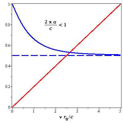
Figure 1: Graphic solution of Eq. (12) for $\tau c/r_{0}=1/5$ and $2\pi\sigma_{0}/c=1/2$.

A substitution of ${\bf A}(0)$ into Eq. (5) readily gives the relaxation rate

$$\nu=\frac{1}{\tau}\left(1-\frac{2\pi\sigma_{0}}{c}\right).$$ (8)

This solution was presented in Ref. Falko89, for $2\pi\sigma_{0}<c$, where it is positive. However it was not mentioned there that it also exists in the case of opposite inequality, which implies an unphysical amplification of the initial current.

To clarify the origin of the negative relaxation rate, we note that a similar system of a small size represents just an $RL$ circuit, in which this rate is positive regardless of the conductance. Therefore it makes sense to start with a 2D conductor of finite size and trace the behaviour of the relaxation rate as its size increases. Consider a conductor in the shape of an infinitely long hollow cylinder of radius $r_{0}$ with a uniform current flowing normally to the axis of the cylinder. Because of the symmetry of the problem, all quantities depend only on the radial distance from this axis, and the vector potential has only the azimuthal component. In the cylindrical coordinate system, Eq. (6) takes up the form

$$\frac{d}{dr}\left[\frac{1}{r}\,\frac{d}{dr}\,(rA_{\varphi})\right]-\frac{\nu^{2}}{c^{2}}\,A_{\varphi}=-\frac{4\pi}{c}\,j_{2}\,\delta(r-r_{0}).$$ (9)

The solution to this equation that is finite at $r=0$ and tends to zero at $r\to\infty$ may be written as

$$A_{\varphi}(r)=a\begin{cases}K_{1}(\nu r_{0}/c)\,I_{1}(\nu r/c),&r<r_{0}\\ I_{1}(\nu r_{0}/c)\,K_{1}(\nu r/c),&r>r_{0},\end{cases}$$ (10)

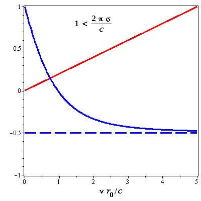
Figure 2: Graphic solution of Eq. (12) for $\tau c/r_{0}=1/5$ and $2\pi\sigma_{0}/c=3/2$.

where $I_{1}$ and $K_{1}$ are the modified Bessel functions of the first and second kind and the coefficient $a$ equals

$$a=\frac{4\pi j_{2}}{\nu}\,\bigl{[}I_{0}(\nu r_{0}/c)\,K_{1}(\nu r_{0}/c)\\ +I_{1}(\nu r_{0}/c)\,K_{0}(\nu r_{0}/c)\bigr{]}^{-1}.$$ (11)

A substitution of Eq. (10) into (5) gives the equation for $\nu$ in the form

$$\nu\tau=1-\frac{4\pi\sigma_{0}}{c}\,{\cal F}(\nu r_{0}/c),$$ (12)

where

$${\cal F}(x)\equiv\frac{I_{1}(x)\,K_{1}(x)}{I_{0}(x)\,K_{1}(x)+I_{1}(x)\,K_{0}(x)}.$$ (13)

This function may be approximated as

$${\cal F}(x)\approx\begin{cases}x/2,&x\ll 1\\ 1/2,&x\gg 1,\end{cases}$$ (14)

so the limiting forms of the solution to Eq. (12) are

$$\nu\approx\begin{cases}\dfrac{1}{\tau}\left(1+\dfrac{2\pi\sigma_{0}}{c}\,\dfrac{r_{0}}{c\tau}\right)^{-1},&\dfrac{c\tau}{r_{0}}+\dfrac{2\pi\sigma_{0}}{c}\gg 1\\ {}&{}\textstyle\\ \dfrac{1}{\tau}\left(1-\dfrac{2\pi\sigma_{0}}{c}\right),&\dfrac{c\tau}{r_{0}}+\dfrac{2\pi\sigma_{0}}{c}\ll 1.\end{cases}$$ (15)

Therefore in the cylindrical geometry, the relaxation rate never becomes negative, no matter how large $r_{0}$ is. If $2\pi\sigma_{0}/c>1$, the relaxation rate tends to zero with increasing $r_{0}$. This suggests that in a presence of dissipation, the transition from finite-size to infinite 2D systems is nontrivial and should be made with caution.

The solution of Eq. (12) may be illustrated by Figures 1 and 2, where the red lines represent linear functions $(\tau c/r_{0})\,x$ and the solid blue curves represent $1-(4\pi\sigma_{0}/c)\,{\cal F}(x)$. The dashed blue lines show the asymptotic values of $1-(4\pi\sigma_{0}/c)\,{\cal F}(\infty)$. The intersections of the red and solid blue lines represent the solutions of Eq. (12) for the hollow cylinder, and their intersections with dashed blue lines present the values of $\nu$ given by Eq. (8) for the infinite plane. Figure 1 corresponds to $2\pi\sigma_{0}/c<1$, and the red line crosses the blue dashed line at $x>0$. As $r_{0}$ increases, the intersection points approach each other and the solutions for the plane and the cylinder merge. Figure 2 corresponds to $2\pi\sigma_{0}/c>1$, and the red line crosses the blue solid line also at $x>0$, so the relaxation rate in the cylinder geometry is always positive. However it obviously intersects the blue dashed line at $x<0$, which corresponds to negative relaxation given by Eq. (8). As $r_{0}$ increases, the actual relaxation rate tends to zero while remaining positive. Hence the straightforward solution of the Drude equation together with the Maxwell equations for a infinite plane instead of a cylinder of infinite radius gives incorrect results.

In Volkov16 , the negative relaxation rate of plasma oscillations was obtained for $k\neq 0$ and $2\pi\sigma_{0}/c\lesssim 1$. However these results were obtained for the case of a rather strong magnetic field, which smears the transition between the $2\pi\sigma_{0}/c>1$ and $2\pi\sigma_{0}/c<1$ regimes. In addition to this, the magnetic field produces a component of current that is uniform in the direction normal to $\bf k$, in which the conductor is also infinite, so the above reasoning applies to this problem as well.

The authors of Volkov16 admit that the electric and magnetic fields do not decay with distance from the conducting plane at the point where the relaxation rate changes sign. This is unphysical and implies that some cutoff parameter should be used. A natural cutoff for such a system is its in-plane size, and the correct treatment of this problem should involve a transition from a finite-size conductor with appropriate in-plane boundary conditions or topology to an infinite one. This would eliminate any unphysical solutions and paradoxical effects.

References

- (1) F. Stern, Phys. Rev. Lett. 18, 546 (1967).
- (2) K. W. Chiu and J. J. Quinn, Phys. Rev. B 9, 4724 (1974).
- (3) V. I. Fal’ko and D. E. Khmel’nitskii, Sov. Phys. JETP 68, 1150 (1989).
- (4) V. A. Volkov and A. A. Zabolotnykh, Phys. Rev. B 94, 165408 (2016); arXiv:1605.00430.