Layerwise Systematic Scan:
Deep Boltzmann Machines and Beyond

Abstract.

For Markov chain Monte Carlo methods, one of the greatest discrepancies between theory and system is the scan order — while most theoretical development on the mixing time analysis deals with random updates, real-world systems are implemented with systematic scans. We bridge this gap for models that exhibit a bipartite structure, including, most notably, the Restricted/Deep Boltzmann Machine. The de facto implementation for these models scans variables in a layer-wise fashion. We show that the Gibbs sampler with a layerwise alternating scan order has its relaxation time (in terms of epochs) no larger than that of a random-update Gibbs sampler (in terms of variable updates). We also construct examples to show that this bound is asymptotically tight. Through standard inequalities, our result also implies a comparison on the mixing times.

1. Introduction

Gibbs sampling, or the Markov chain Monte Carlo method in general, plays a central role in machine learning and have been widely implemented as the backbone algorithm for models such as Deep Boltzmann Machines (Salakhutdinov and Hinton, 2009), latent Dirichlet allocations (Blei et al., 2003), and factor graphs in general. Given a set of random variables and a target distribution $\pi$, the Gibbs sampler iteratively updates one variable at a time according to the distribution $\pi$ conditioned on the values of all other variables. If the ergodicity condition is met, then the Gibbs sampler eventually converges to the target distribution.

There are two ways to choose which variable to update at the next iteration: (1) Random Update, where in each epoch (or round) one variable is picked uniformly at random with replacement; and (2) Systematic Scan, where in each epoch all variables are updated using some pre-determined order. Although most theoretical development on analyzing Gibbs sampling deals with random updates (Jerrum, 2003; Levin et al., 2009), systematic scans are prevalent in real-world implementations due to their hardware-friendly nature (cache locality for factor graphs, SIMD for Deep Boltzmann Machines, etc.). It is natural to wonder, whether using systematic scan, rather than random updates, would delay the mixing time, the number of iterations the Gibbs sampler requires to reach the target distribution.

The mixing time of these two update strategies can differ by some high polynomial factors in either directions (He et al., 2016; Roberts and Rosenthal, 2015). Even more pathological examples were constructed for non-Gibbs Markov chains such that systematic scan is not even ergodic whereas the random-update sampler is rapidly mixing (Dyer et al., 2008). Indeed, even for a system as simple as the Ising model, a comparison result remains elusive (Levin et al., 2009, Open problem 5, p. 300). As a consequence, theoretical results on rapidly mixing, such as (Bubley and Dyer, 1997; Mossel and Sly, 2013), do not readily apply to the scan algorithms used in practice.

1.1. Main results.

In this paper, we bridge this gap between theory and system. We focus on bipartite distributions, in which variables can be divided into two partitions — conditioned on one of the partitions, variables from the other partition are mutually independent. This bipartite structure arises naturally in practice, including Restricted/Deep Boltzmann Machines. For a bipartite distribution, the de facto implementation is that in each epoch, we scan all variables from one of the partitions first, and then the other. We call this the alternating-scan sampler. Note that in order to define a valid Markov chain, we have to consider systematic scans in epochs, in which all variables are updated once. Our main theorem is the following.

Theorem 1 (Main Theorem).

For any bipartite distribution $\pi$, if the random-update Gibbs sampler is ergodic, then so is the alternating-scan sampler. Moreover, the relaxation time of the alternating-scan sampler (in terms of epochs) is no larger than that of the random-update one (in terms of variable updates).

The relaxation time (inverse spectral gap) measures the mixing time from a “warm” start. It is closely related to the (total variation distance) mixing time, and governs mixing times under other metrics as well (Levin et al., 2009). Through standard inequalities, Theorem 1 also implies a comparison result in terms of mixing times, Corollary 10. As we count epochs in Theorem 1, the alternating-scan sampler is implicitly slower by a factor of $n$, the number of variables. We also show that Theorem 1 is asymptotically tight via Example 11. Thus this implicit factor $n$ slowdown cannot be improved in general.

More specifically, we summarize our contribution as follows.

1. In Section 4, we establish Theorem 1. By focusing on bipartite systems, we are able to obtain much stronger result than recent studies in the more general setting (He et al., 2016). We note that standard Markov chain comparison results, such as (Diaconis and Saloff-Coste, 1993), do not seem to fit into our setting. Instead, we give a novel analysis via estimates of operator norms of certain carefully defined matrices. One key observation is to consider an artificial but equivalent variant of the alternating-scan sampler, where we insert an extra random update between updating variables from the two partitions. This does not change the algorithm since the extra random update is either redundant with the updates in the first partition or with those in the second.

2. In Section 5, we discuss bipartite distributions that arise naturally in machine learning. In particular, our result is a rigorous justification of the popular layer-wise scan sampler for Deep Boltzmann Machines (Salakhutdinov and Hinton, 2009). Our result also applies to other models such as Restricted Boltzmann Machines (Smolensky, 1986) and, more generally, any bipartite factor graph.

3. In Section 6, we conduct experiments to verify our theory and analyze the gap between our worst case theoretical bound and numerical evidences. We observe that in the rapidly mixing regime, the alternating-scan sampler is usually faster than the random-update one, whereas in the slow mixing regime, the alternating-scan sampler can be slower by a factor $O(n)$. We hope these observations shed some light on more fine-grained comparison bounds in the future.

2. Related Work

Probably the most relevant work is the recent analysis conducted by He et al. (2016) about the impact of the scan order on the mixing time of the Gibbs sampling. They (1) constructed a variety of models in which the scan order can change the mixing time significantly in several different ways and (2) proved comparison results on the mixing time between random updates and a variant of systematic scans where “lazy” moves are allowed. In this paper, we focus on a more specific case, i.e., bipartite systems, and so our bound is stronger — in fact, our bound can be exponentially stronger when the underlying chain is torpidly mixing. Moreover, our result does not modify the standard scan algorithm.

Another related work is the recent analysis by Tosh (2016) considering the mixing time of an alternating sampler for the Restricted Boltzmann Machine (RBM). Tosh showed that, under Dobrushin-like conditions (Dobrushin, 1970), i.e., when the weights in the RBM are sufficiently small, the alternating sampler mixes rapidly. For models other than RBM, mixing time results for systematic scans are relatively rare. Known examples are usually restricted to very specific models (Diaconis and Ram, 2000) or under conditions to ensure that the correlations are sufficiently weak (Dyer et al., 2006; Hayes, 2006; Dyer et al., 2008). Typical conditions of this sort are variants of the classical Dobrushin condition (Dobrushin, 1970). See also (Blanca et al., 2018) for very recent results on analyzing the alternating scan sampler (among others) on the 2D grid under conditions of the Dobrushin-type. In contrast, our work focuses on the relative performance between random updates and systematic scan, and does not rely on Dobrushin-like conditions. In particular, our results extend to the torpid mixing regime as well as the rapid mixing one.

Our primary focus is on discrete state spaces. The scan order question has also been asked and explored in general state spaces. Despite a long line of research (Hastings, 1970; Peskun, 1973; Caracciolo et al., 1990; Liu et al., 1995; Roberts and Sahu, 1997; Roberts and Rosenthal, 1997; Tierney, 1998; Maire et al., 2014; Roberts and Rosenthal, 2015; Andrieu, 2016), to the best of our knowledge, no decisive answer is known.

Another line of related research is about the scan order in stochastic gradient descent (Recht and Ré, 2012; Shamir, 2016; Gürbüzbalaban et al., 2017). Our setting in this paper is very different and the techniques are different as well.

3. Preliminaries on Markov Chains

Let $\Omega$ be a discrete state space and $P$ be a $\left|\Omega\right|$-by-$\left|\Omega\right|$ stochastic matrix describing a (discrete time) Markov chain on $\Omega$. The matrix $P$ is also called the transition matrix or the kernel of the chain. Thus, $P^{t}(\sigma_{0},\cdot)$ is the distribution of the chain at time $t$ starting from $\sigma_{0}$. Let $\pi(\cdot)$ be a stationary distribution of $P$. The Markov chain defined by $P$ is reversible (with respect to $\pi(\cdot)$) if $P$ satisfies the detailed balance condition:

(1) $$\pi(\sigma)P(\sigma,\tau)=\pi(\tau)P(\tau,\sigma)$$

for any $\sigma,\tau\in\Omega$. We note that in general the systematic scan sampler is not reversible. The Markov chain is called irreducible if $P$ connects the whole state space $\Omega$, namely, for any $\sigma,\tau\in\Omega$, there exists $t$ such that $P^{t}(\sigma,\tau)>0$. It is called aperiodic if $\gcd\{t>0:P^{t}(\sigma,\sigma)>0\}=1$ for every $\sigma\in\Omega$. We call $P$ ergodic if it is both irreducible and aperiodic. An ergodic Markov chain converges to its unique stationary distribution (Levin et al., 2009).

The total variation distance $\left\|\cdot\right\|_{TV}$ for two distributions $\mu$ and $\nu$ on $\Omega$ is defined as

$$\left\|\mu-\nu\right\|_{TV}=\max_{A\subset\Omega}\left|\mu(A)-\nu(A)\right|=\frac{1}{2}\sum_{\sigma\in\Omega}\left|\mu(\sigma)-\nu(\sigma)\right|.$$

The mixing time $T_{mix}$ is defined as

$$T_{mix}(P):=\min\left\{t\geq 0:\max_{\sigma\in\Omega}\left\|P^{t}(\sigma,\cdot)-\pi\right\|_{TV}\leq\frac{1}{2e}\right\},$$

where the choice of the constant $\frac{1}{2e}$ is merely for convenience and is not significant (Levin et al., 2009).

When $P$ is ergodic and reversible, the eigenvalues $(\xi_{i})_{i\in[\left|\Omega\right|]}$ of $P$ satisfies $-1<\xi_{i}\leq 1$, and additionally, $Pf=f$ if and only if $f$ is constant (see (Levin et al., 2009, Lemma 12.1)). The spectral gap of $P$ is defined by

$$\lambda(P):=1-\max\{\left|\xi\right|:\xi\text{ is an eigenvalue of $P$}$$

(2) $$\hskip 28.45274pt\text{ and $\xi\neq 1$}\}.$$

The relaxation time for a reversible $P$ is defined as

(3) $$T_{rel}(P):=\lambda(P)^{-1}.$$

The relaxation time and the mixing time differ by at most a factor of $\log\left(\frac{2e}{\pi_{min}}\right)$ where $\pi_{min}=\min_{\sigma\in\Omega}\pi(\sigma)$, shown by the following theorem (see, for example, (Levin et al., 2009, Theorem 12.4 and 12.5)). In fact, the relaxation time governs mixing properties with respect to metrics other than the total variation distance as well. See (Levin et al., 2009, Chapter 12) for more details.

Theorem 2.

Let $P$ be the transition matrix of a reversible and ergodic Markov chain with the state space $\Omega$ and the stationary distribution $\pi$. Then

$$T_{rel}(P)-1\leq T_{mix}(P)\leq T_{rel}(P)\log\left(\frac{2e}{\pi_{min}}\right),$$

where $\pi_{min}=\min_{\sigma\in\Omega}\pi(\sigma)$.

The factor $\log\pi_{min}^{-1}$ is usually linear in $n$, the number of variables, in the context of Gibbs sampling which is our primary focus later. Theorem 2 is tight, and there is no good way of avoiding losing this $\log\pi_{min}^{-1}$ factor in general, with the spectral method.

Unfortunately, the systematic-scan sampler is not reversible, and therefore Theorem 2 does not apply. Instead, we use an extension developed by Fill (1991). For a non-reversible transition matrix $P$, let the multiplicative reversiblization be $R(P):=PP^{*}$, where $P^{*}$ is the adjoint of $P$ defined as

(4) $$P^{*}(\sigma,\tau)=\frac{\pi(\tau)P(\tau,\sigma)}{\pi(\sigma)}.$$

Then $R(P)$ is reversible. Let the relaxation time for a (not necessarily reversible) $P$ be

(5) $$T_{rel}(P):=\frac{1}{1-\sqrt{1-\lambda(R(P))}}.$$

In particular, if $P$ is reversible, then (5) recovers (3) (see Proposition 4). In general, the multiplicative reversibilization mixes similarly to the original non-reversible chain. See (Fill, 1991) for more details.

The following theorem is a simple consequence of (Fill, 1991, Theorem 2.1).

Theorem 3.

Let $P$ be the transition matrix of an ergodic Markov chain with the state space $\Omega$ and the stationary distribution $\pi$. Then

$$T_{mix}(P)\leq\log\left(\frac{4e^{2}}{\pi_{min}}\right)T_{rel}(P),$$

where $\pi_{min}=\min_{\sigma\in\Omega}\pi(\sigma)$.

Note that our definition of relaxation times (5) for non-reversible Markov chains yields asymptotically the same upper bound in Theorem 2.

Proof of Theorem 3.

We first restate (Fill, 1991, Theorem 2.1) (note that the norm in (Fill, 1991) is twice the total variation distance):

(6) $$\left\|P^{t}(\sigma,\cdot)-\pi\right\|_{TV}^{2}\leq\frac{\left(1-\lambda(R(P))\right)^{t}}{\pi(\sigma)}.$$

Let $\lambda:=\lambda(R(P))$ and $T:=\log\left(\frac{4e^{2}}{\pi_{\min}}\right)T_{rel}(P)=\frac{1}{1-\sqrt{1-\lambda}}\log\left(\frac{4e^{2}}{\pi_{\min}}\right)$. Then it is easy to verify that

$$T\geq\frac{2}{\lambda}\log\left(\frac{2e}{\sqrt{\pi_{\min}}}\right)$$

and by (6), we have that

$$\max_{\sigma\in\Omega}\left\|P^{T}(\sigma,\cdot)-\pi\right\|_{TV} \leq\frac{\left(1-\lambda\right)^{T/2}}{\sqrt{\pi_{\min}}}$$

$$\leq\frac{\left(1-\lambda\right)^{\lambda^{-1}\log\left(\frac{2e}{\sqrt{\pi_{\min}}}\right)}}{\sqrt{\pi_{\min}}}$$

$$\leq\frac{e^{-\log\left(\frac{2e}{\sqrt{\pi_{\min}}}\right)}}{\sqrt{\pi_{\min}}}$$

$$=\frac{1}{2e}.$$

In other words,

$$T_{mix}(P)\leq T =\log\left(\frac{4e^{2}}{\pi_{\min}}\right)T_{rel}(P).\qed$$

3.1. Operator Norms and the Spectral Gap

We also view the transition matrix $P$ as an operator that mapping functions to functions. More precisely, let $f$ be a function $f:\Omega\rightarrow\mathbb{R}$ and $P$ acting on $f$ is defined as

$$Pf(x):=\sum_{y\in\Omega}P(x,y)f(y).$$

This is also called the Markov operator corresponding to $P$. We will not distinguish the matrix $P$ from the operator $P$ as it will be clear from the context. Note that $Pf(x)$ is the expectation of $f$ with respect to the distribution $P(x,\cdot)$. We can regard a function $f$ as a column vector in $\mathbb{R}^{\Omega}$, in which case $Pf$ is simply matrix multiplication. Recall (4) and $P^{*}$ is also called the adjoint operator of $P$. Indeed, $P^{*}$ is the (unique) operator that satisfies $\langle f,Pg\rangle_{\pi}=\langle P^{*}f,g\rangle_{\pi}$. It is easy to verify that if $P$ satisfies the detailed balanced condition (1), then $P$ is self-adjoint, namely $P=P^{*}$.

The Hilbert space $L_{2}(\pi)$ is given by endowing $\mathbb{R}^{\Omega}$ with the inner product

$$\langle f,g\rangle_{\pi}:=\sum_{x\in\Omega}f(x)g(x)\pi(x),$$

where $f,g\in\mathbb{R}^{\Omega}$. In particular, the norm in $L_{2}(\pi)$ is given by

$$\left\|f\right\|_{\pi}:=\langle f,f\rangle_{\pi}.$$

The spectral gap (3) can be rewritten in terms of the operator norm of $P$, which is defined by

$$\left\|P\right\|_{\pi}:=\max_{\left\|f\right\|_{\pi}\neq 0}\frac{\left\|Pf\right\|_{\pi}}{\left\|f\right\|_{\pi}}.$$

Indeed, the operator norm equals the largest eigenvalue (which is just $1$ for a transition matrix $P$), but we are interested in the second largest eigenvalue. Define the following operator

(7) $$S_{\pi}(\sigma,\tau):=\pi(\tau).$$

It is easy to verify that $S_{\pi}f(\sigma)=\langle f,\mathbf{1}\rangle_{\pi}$ for any $\sigma$. Thus, the only eigenvalues of $S_{\pi}$ are $0$ and $1$, and the eigenspace of eigenvalue $0$ is $\{f\in L_{2}(\pi):\langle f,\mathbf{1}\rangle_{\pi}=0\}$. This is exactly the union of eigenspaces of $P$ excluding the eigenvalue $1$. Hence, the operator norm of $P-S_{\pi}$ equals the second largest eigenvalue of $P$, namely,

(8) $$\lambda(P)=1-\left\|P-S_{\pi}\right\|_{\pi}.$$

The expression in (8) can be found in, for example, (Ullrich, 2014, Eq. (2.8)). In particular, using (8), we show that the definition (5) coincides with (3) when $P$ is reversible.

Proposition 4.

Let $P$ be the transition matrix of a reversible matrix with the stationary distribution $\pi$. Then

$$\frac{1}{\lambda(P)}=\frac{1}{1-\sqrt{1-\lambda(R(P))}}.$$

Proof.

Since $P$ is reversible, $P$ is self-adjoint, namely, $P^{*}=P$. Hence $\left(P-S_{\pi}\right)^{*}=P^{*}-S_{\pi}$ and

$$\left(P-S_{\pi}\right)\left(P-S_{\pi}\right)^{*} =\left(P-S_{\pi}\right)\left(P^{*}-S_{\pi}\right)$$

$$=PP^{*}-PS_{\pi}-S_{\pi}P^{*}+S_{\pi}S_{\pi}$$

$$=PP^{*}-S_{\pi},$$

where we use the fact that $PS_{\pi}=S_{\pi}P^{*}=S_{\pi}S_{\pi}=S_{\pi}$. It implies that

(by (8)) $$1-\lambda(R(P)) =\left\|R(P)-S_{\pi}\right\|_{\pi}$$

$$=\left\|PP^{*}-S_{\pi}\right\|_{\pi}$$

$$=\left\|\left(P-S_{\pi}\right)\left(P-S_{\pi}\right)^{*}\right\|_{\pi}$$

$$=\left\|P-S_{\pi}\right\|_{\pi}^{2}$$

$$=\left(1-\lambda(P)\right)^{2}.$$

Rearranging the terms yields the claim. ∎

4. Alternating Scan

In this section we describe the random update and the alternating scan sampler, and compare these two. Let $V=\{x_{1},\dots,x_{n}\}$ be a set of variables where each variable takes values from some finite set $S$. Let $\pi(\cdot)$ be a distribution defined on $S^{V}$.

Let $\sigma\in S^{V}$ be a configuration, namely $\sigma:V\to S$. Let $\sigma^{x,s}$ be the configuration that agrees with $\sigma$ except at $x$, where $\sigma^{x,s}(x)=s$ for $s\in S$. In other words, for any $y\in V$,

$$\sigma^{x,s}(y):=\begin{cases}\sigma(y)&\textrm{if $y\neq x$};\\ s&\textrm{if $y=x$}.\end{cases}$$

Algorithm 1 Gibbs sampling with random updates

0:  Starting configuration $\sigma=\sigma_{0}$

  for $t=1,\dots,T_{mix}$ do

     With probability $1/2$, do nothing.

     Otherwise, select a variable $x\in V$ uniformly at random.

     Set $\sigma\leftarrow\sigma^{x,s}$ with probability $\frac{\pi(\sigma^{x,s})}{\sum_{t\in S}\pi(\sigma^{x,t})}$.

  end for

  return  $\sigma$

The lazy Gibbs sampler is defined in Algorithm 1. Let $n=\left|V\right|$ be the total number of variables. The transition kernel $P_{RU}$ (where RU stands for “random updates”) of the sampler in Algorithm 1 is defined as:

$$P_{RU}(\sigma,\tau)=\begin{cases}\frac{1}{2n}\cdot\frac{\pi(\sigma^{x,s})}{\sum_{t\in S}\pi(\sigma^{x,t})}&\textrm{ if }\tau\neq\sigma\textrm{ and there are $x\in V$}\\ &\textrm{ and $s\in S$ such that }\tau=\sigma^{x,s};\\ 1/2+\sum_{x\in V}\frac{1}{2n}\cdot\frac{\pi(\sigma^{x,\sigma(x)})}{\sum_{t\in S}\pi(\sigma^{x,t})}&\textrm{ if }\tau=\sigma;\\ 0&\textrm{ otherwise,}\end{cases}$$

where $\sigma,\tau$ are two configurations. It is not hard to see, for example, by checking the detailed balance condition (1), that $\pi(\cdot)$ is the stationary distribution of $P_{RU}$. Note that this Markov chain is lazy, i.e., it remains at its current state with probability at least $1/2$. This self-loop probability is higher than $1/2$ because when we update a variable there is positive probability of no change. Lazy chains are often studied in the literature because of its technical conveniences. The self-loop eliminates potential periodicity, and all eigenvalues of a lazy chain are non-negative. In the context of Gibbs sampling, these are merely artifacts of the available techniques and considering the lazy version is not really necessary (Rudolf and Ullrich, 2013; Dyer et al., 2014). Our main result actually applies to both lazy and non-lazy versions. See the remarks after the proof of Theorem 1.

Our main focus is bipartite distributions, defined next. These distributions arise naturally from bipartite factor graphs, including, most notably, Restricted Boltzmann Machines.

Definition 5.

The joint distribution $\pi(\cdot)$ of random variables $V=\{x_{1},\dots,x_{n}\}$ is bipartite, if $V$ can be partitioned into two sets $V_{1}$ and $V_{2}$ $($namely $V_{1}\cup V_{2}=V$ and $V_{1}\cap V_{2}=\emptyset)$, such that conditioned on any assignment of variables in $V_{2}$, all variables in $V_{1}$ are mutually independent, and vice versa.

In the following we consider a particular systematic scan sampler for bipartite distributions. For a configuration $\sigma$, let $\sigma_{i}:=\sigma|_{V_{i}}$ be its projection on $V_{i}$ where $i=1,2$. The alternating-scan sampler is given in Algorithm 2, where $n_{1}=\left|V_{1}\right|$ and $n_{2}=\left|V_{2}\right|$.

Algorithm 2 Alternating-scan sampler

0:  Starting configuration $\sigma=\sigma_{0}$

  for $t=1,\dots,T_{mix}$ do

     for $i=1,\dots,n_{1}$ do

        Set $\sigma\leftarrow\sigma^{x_{i},s}$ with probability $\frac{\pi(\sigma^{x_{i},s})}{\sum_{t\in S}\pi(\sigma^{x_{i},t})}$.

     end for

     for $j=1,\dots,n_{2}$ do

        Set $\sigma\leftarrow\sigma^{y_{j},s}$ with probability $\frac{\pi(\sigma^{y_{j},s})}{\sum_{t\in S}\pi(\sigma^{y_{j},t})}$.

     end for

  end for

  return  $\sigma$

In other words, the alternating-scan sampler sequentially resamples all variables in $V_{1}$, and then resamples all variables in $V_{2}$. Note that since we are considering a bipartite distribution, in order to resample $x_{i}\in V_{1}$, we only need to condition on $\sigma_{2}$. In other words, for any $i\in[n_{1}]$, the distribution $\left(\frac{\pi(\sigma^{x_{i},s})}{\sum_{t\in S}\pi(\sigma^{x_{i},t})}\right)_{s\in S}$ that we draws from depends only on $\sigma_{2}$. Similarly, resampling $y_{j}\in V_{2}$ only depends on $\sigma_{1}$. We will denote the transition kernel of the alternating-scan sampler as $P_{AS}$, where AS stands for “alternating scan”.

An unusual feature of systematic-scan samplers (including the alternating-scan sampler) is that they are not reversible. Namely the detailed balance condition (1) does not in general hold. This is because updating variables $x$ and $y$ in order is in general different from updating $y$ and $x$ in order. This imposes a technical difficulty as most of the theoretical tools of analyzing these chains are not suitable for irreversible chains, such as the Dirichlet form (Diaconis and Saloff-Coste, 1993) or conductance bounds (Jerrum and Sinclair, 1993; Sinclair, 1992).

On the other hand, the scan sampler is aperiodic. Any potential state $\sigma$ of the chain must be in the state space $\Omega$. Therefore $\pi(\sigma)>0$ and the probability of staying in $\sigma$ is strictly positive. Moreover, if the Gibbs sampler is irreducible (namely the state space $\Omega$ is connected via single variable flips), then so is the scan sampler. This is because any single variable update can be simulated in the scan sampler, with small but strictly positive probability. Hence if the Gibbs sampler is ergodic, then so is the scan sampler.

We restate our main theorem here in formal terms.

Theorem 1.

For any bipartite distribution $\pi$, if $P_{RU}$ is ergodic, then so is $P_{AS}$. Moreover,

$$T_{rel}(P_{AS})\leq T_{rel}(P_{RU}).$$

We will prove Theorem 1 next. The transition matrix of updating a particular variable $x$ is the following

(9) $$T_{x}(\sigma,\tau)=\begin{cases}\frac{\pi(\sigma^{x,s})}{\sum_{s\in S}\pi(\sigma^{x,s})}&\textrm{if }\tau=\sigma^{x,s}\textrm{ for some $s\in S$};\\ 0&\textrm{otherwise.}\\ \end{cases}$$

Moreover, let $I$ be the identity matrix that $I(\sigma,\tau)=\mathbbm{1}(\sigma,\tau)$.

Lemma 6.

Let $\pi$ be a bipartite distribution, and $P_{RU}$, $P_{AS}$, $T_{x}$ be defined as above. Then we have that

1. $\displaystyle P_{RU}=\frac{I}{2}+\frac{1}{2n}\sum_{x\in V}T_{x}$;

2. $\displaystyle P_{AS}=\prod_{i=1}^{n_{1}}T_{x_{i}}\prod_{j=1}^{n_{2}}T_{y_{j}}$.

Proof.

Note that $T_{x}$ is the transition matrix of resampling $\sigma(x)$. For $P_{RU}$, the term $\frac{I}{2}$ comes from the fact that the chain is “lazy”. With the other $1/2$ probability, we resample $\sigma(x)$ for a uniformly chosen $x\in V$. This explains the term $\frac{1}{2n}\sum_{x\in V}T_{x}$.

For $P_{AS}$, we sequentially resample all variables in $V_{1}$ and then all variables in $V_{2}$, which yields the expression. ∎

Lemma 7.

Let $\pi$ be a bipartite distribution and $T_{x}$ be defined as above. Then we have that

1. For any $x\in V$, $T_{x}$ is a self-adjoint operator and idempotent. Namely, $T_{x}=T_{x}^{*}$ and $T_{x}T_{x}=T_{x}$.

2. For any $x\in V$, $\left\|T_{x}\right\|_{\pi}=1$.

3. For any $x,x^{\prime}\in V_{i}$ where $i=1$ or $2$, $T_{x}$ and $T_{x^{\prime}}$ commute. In other words $T_{x^{\prime}}T_{x}=T_{x}T_{x^{\prime}}$ if $x,x^{\prime}\in V_{i}$ for $i=1$ or $2$.

Proof.

For Item 1, the fact that $T_{x}$ is self-adjoint follows from the detailed balance condition (1). Idempotence is because updating the same vertex twice is the same as a single update.

Item 2 follows from Item 1. This is because

$$\left\|T_{x}\right\|_{\pi}=\left\|T_{x}T_{x}\right\|_{\pi}=\left\|T_{x}T_{x}^{*}\right\|_{\pi}=\left\|T_{x}\right\|_{\pi}^{2}.$$

For Item 3, suppose $i=1$. Since $\pi$ is bipartite, resampling $x$ or $x^{\prime}$ only depends on $\sigma_{2}$. Therefore the ordering of updating $x$ or $x^{\prime}$ does not matter as they are in the same partition. ∎

Define

$$P_{GS1}:=\frac{I}{2}+\frac{1}{2n_{1}}\sum_{i=1}^{n_{1}}T_{x_{i}},\text{\quad\quad and \quad\quad}P_{GS2}:=\frac{I}{2}+\frac{1}{2n_{2}}\sum_{j=1}^{n_{2}}T_{y_{j}}.$$

Then, since $n_{1}+n_{2}=n$,

(10) $$P_{RU}=\frac{1}{n}\left(n_{1}P_{GS1}+n_{2}P_{GS2}\right).$$

Similarly, define

$$P_{AS1}:=\prod_{i=1}^{n_{1}}T_{x_{i}},\text{\quad\quad and \quad\quad}P_{AS2}:=\prod_{j=1}^{n_{2}}T_{y_{j}}.$$

Then

(11) $$P_{AS}=P_{AS1}P_{AS2}.$$

With this notation, Lemma 7 also implies the following.

Corollary 8.

The following holds:

1. $\left\|P_{AS1}\right\|_{\pi}\leq 1$ and $\left\|P_{AS2}\right\|_{\pi}\leq 1$.

2. $P_{AS1}P_{GS1}=P_{AS1}$ and $P_{GS2}P_{AS2}=P_{AS2}$.

Proof.

For Item 1, by the submultiplicity of operator norms:

$$\left\|P_{AS1}\right\|_{\pi} =\left\|\prod_{i=1}^{n_{1}}T_{x_{i}}\right\|_{\pi}\leq\prod_{i=1}^{n_{1}}\left\|T_{x_{i}}\right\|_{\pi}$$

(By Item 2 of Lemma 7) $$=1.$$

The claim $\left\|P_{AS2}\right\|_{\pi}\leq 1$ follows similarly.

Item 2 follows from Item 1 and 3 of Lemma 7. We verify the first case as follows.

$$P_{AS1}P_{GS1} =\prod_{i=1}^{n_{1}}T_{x_{i}}\left(\frac{I}{2}+\frac{1}{2n_{1}}\sum_{j=1}^{n_{1}}T_{x_{j}}\right)$$

$$=\frac{1}{2}\cdot\prod_{i=1}^{n_{1}}T_{x_{i}}+\frac{1}{2n_{1}}\cdot\prod_{i=1}^{n_{1}}T_{x_{i}}\sum_{j=1}^{n_{1}}T_{x_{j}}$$

$$=\frac{1}{2}\cdot\prod_{i=1}^{n_{1}}T_{x_{i}}+\frac{1}{2n_{1}}\cdot\sum_{j=1}^{n_{1}}T_{x_{j}}\prod_{i=1}^{n_{1}}T_{x_{i}}$$

(By Item 3 of Lemma 7) $$=\frac{1}{2}\cdot\prod_{i=1}^{n_{1}}T_{x_{i}}+\frac{1}{2n_{1}}\cdot\sum_{j=1}^{n_{1}}T_{x_{1}}T_{x_{2}}\cdots T_{x_{j}}T_{x_{j}}\cdots T_{x_{n_{1}}}$$

(By Item 1 of Lemma 7) $$=\frac{1}{2}\cdot\prod_{i=1}^{n_{1}}T_{x_{i}}+\frac{1}{2n_{1}}\cdot\sum_{j=1}^{n_{1}}\prod_{i=1}^{n_{1}}T_{x_{i}}$$

$$=\frac{1}{2}\cdot\prod_{i=1}^{n_{1}}T_{x_{i}}+\frac{1}{2}\cdot\prod_{i=1}^{n_{1}}T_{x_{i}}$$

$$=P_{AS1}.$$

The other case is similar. ∎

Item 2 of Corollary 8 captures the following intuition: if we sequentially update all variables in $V_{i}$ for $i=1,2$, then an extra individual update either before or after does not change the distribution. Recall Eq. (5).

Lemma 9.

Let $\pi$ be a bipartite distribution and $P_{RU}$ and $P_{AS}$ be defined as above. Then we have that

$$\left\|R(P_{AS})-S_{\pi}\right\|_{\pi}\leq\left\|P_{RU}-S_{\pi}\right\|_{\pi}^{2}.$$

Proof.

Recall (7), the definition of $S_{\pi}$, using which it is easy to see that

(12) $$P_{AS1}S_{\pi}=S_{\pi}P_{AS2}=S_{\pi}S_{\pi}=S_{\pi}.$$

Thus,

(By (10)) $$P_{AS1}(P_{RU}-S_{\pi})P_{AS2} =P_{AS1}\left(\frac{n_{1}}{n}P_{GS1}+\frac{n_{2}}{n}P_{GS2}-S_{\pi}\right)P_{AS2}$$

$$=\frac{n_{1}}{n}P_{AS1}P_{GS1}P_{AS2}+\frac{n_{2}}{n}P_{AS1}P_{GS2}P_{AS2}-P_{AS1}S_{\pi}P_{AS2}$$

(By Item 2 of Cor 8) $$=\frac{n_{1}}{n}P_{AS1}P_{AS2}+\frac{n_{2}}{n}P_{AS1}P_{AS2}-S_{\pi}$$

$$=P_{AS1}P_{AS2}-S_{\pi}$$

(13) $$=P_{AS}-S_{\pi},$$

where in the last step we use (11). Moreover, we have that

$$P_{AS}^{*} =\left(\prod_{i=1}^{n_{1}}T_{x_{i}}\prod_{j=1}^{n_{2}}T_{y_{j}}\right)^{*}$$

$$=\prod_{j=1}^{n_{2}}T_{y_{n_{2}+1-j}}^{*}\prod_{i=1}^{n_{1}}T_{x_{n_{1}+1-i}}^{*}$$

(By Item 1 of Lemma 7) $$=\prod_{j=1}^{n_{2}}T_{y_{n_{2}+1-j}}\prod_{i=1}^{n_{1}}T_{x_{n_{1}+1-i}}$$

(By Item 3 of Lemma 7) $$=\prod_{j=1}^{n_{2}}T_{y_{j}}\prod_{i=1}^{n_{1}}T_{x_{i}}$$

$$=P_{AS2}P_{AS1}.$$

Hence, similarly to (13), we have that

$$P_{AS2}(P_{RU}-S_{\pi})P_{AS1} =P_{AS2}P_{AS1}-S_{\pi}$$

(14) $$=P_{AS}^{*}-S_{\pi}.$$

Using (12), we further verify that

$$\left(P_{AS}-S_{\pi}\right)\left(P_{AS}^{*}-S_{\pi}\right) =P_{AS}P_{AS}^{*}-P_{AS}S_{\pi}-S_{\pi}P_{AS}^{*}+S_{\pi}S_{\pi}$$

(15) $$=P_{AS}P_{AS}^{*}-S_{\pi}$$

Combining (13), (14), and (15), we see that

$$\left\|R(P_{AS})-S_{\pi}\right\|_{\pi} =\left\|P_{AS}P_{AS}^{*}-S_{\pi}\right\|_{\pi}$$

$$=\left\|\left(P_{AS}-S_{\pi}\right)\left(P_{AS}^{*}-S_{\pi}\right)\right\|_{\pi}$$

$$=\left\|P_{AS1}\left(P_{RU}-S_{\pi}\right)P_{AS2}P_{AS2}\left(P_{RU}-S_{\pi}\right)P_{AS1}\right\|_{\pi}$$

$$\leq\left\|P_{AS1}\right\|_{\pi}\left\|P_{RU}-S_{\pi}\right\|_{\pi}\left\|P_{AS2}\right\|_{\pi}\left\|P_{AS2}\right\|_{\pi}\left\|P_{RU}-S_{\pi}\right\|_{\pi}\left\|P_{AS1}\right\|_{\pi}$$

$$\leq\left\|P_{RU}-S_{\pi}\right\|_{\pi}^{2},$$

where the first inequality is due to the submultiplicity of operator norms, and we use Item 1 of Corollary 8 in the last line. ∎

Remark.

The last inequality in the proof of Lemma 9 crucially uses the fact that the distribution is bipartite. If there are, say, $k$ partitions, then the corresponding operators $P_{AS1},\dots,P_{ASk}$ do not commute and the proof does not generalize.

Proof of Theorem 1.

For the first part, notice that the alternating-scan sampler is aperiodic. Any possible state $\sigma$ of the chain must be in the state space $\Omega$. Therefore $\pi(\sigma)>0$ and the probability of staying at $\sigma$ is strictly positive. Moreover, any single variable update can be simulated in the scan sampler, with small but strictly positive probability. Hence if the random-update sampler is irreducible, then so is the scan sampler.

To show that $T_{rel}(P_{AS})\leq T_{rel}(P_{RU})$, we have the following

(By (5)) $$T_{rel}(P_{AS}) =\frac{1}{1-\sqrt{1-\lambda(R(P_{AS}))}}$$

(By (8)) $$=\frac{1}{1-\sqrt{\left\|R(P_{AS})-S_{\pi}\right\|_{\pi}}}$$

(By Lemma 9) $$\leq\frac{1}{1-\left\|P_{RU}-S_{\pi}\right\|_{\pi}}$$

(By (8)) $$=\frac{1}{\lambda(P_{RU})}$$

(By (3)) $$=T_{rel}(P_{RU}).$$

This completes the proof. ∎

Remark.

It is easy to check that the proof also works if we consider the non-lazy version of $P_{RU}$. To do so, we just replace $\frac{I}{2}+\frac{1}{2n}\sum_{x\in V}T_{x}$ with $\frac{1}{n}\sum_{x\in V}T_{x}$ and the rest of the proof goes through without changes.

Remark.

Our argument can also handle the case of general state spaces, such as Gaussian variables, since the essential property we use is the commutativity of updating variables from the same partition. For general state spaces, in order to apply Theorem 1 on mixing times, we need to replace Theorem 2 and Theorem 3 with their continuous counterparts. See for example (Lawler and Sokal, 1988).

Using Theorem 2 and Theorem 3, we translate Theorem 1 in terms of the mixing time.

Corollary 10.

For a Markov random field defined on a bipartite graph, let $P_{RU}$ and $P_{AS}$ be the transition kernels of the random-update Gibbs sampler and the alternating-scan sampler, respectively. Then,

$$T_{mix}(P_{AS})\leq\log\left(\frac{4e^{2}}{\pi_{min}}\right)\left(T_{mix}(P_{RU})+1\right),$$

where $\pi_{min}=\min_{\sigma\in\Omega}\pi(\sigma)$.

Since $n$ variables are updated in each epoch of $P_{AS}$, one might hope to strengthen Theorem 1 so that $nT_{rel}(P_{AS})$ is also no larger than $T_{rel}(P_{RU})$. Unfortunately, this is not the case and we give an example (similar to the “two islands” example due to He et al. (2016)) where $T_{mix}(P_{AS})\asymp T_{mix}(P_{RU})$ and $T_{rel}(P_{AS})\asymp T_{rel}(P_{RU})$. This example implies that Theorem 1 is asymptotically tight. However, it is still possible that Corollary 10 is loose by a factor of $\log\pi_{min}^{-1}$. This potential looseness is difficult to circumvent due to the spectral approach we took.

Example 11.

Let $G=(L\cup R,E)$ be a complete bipartite graph $K_{n,n}$ and we want to sample an uniform independent set in $G$. In other words, each vertex is a Boolean variable and a valid configuration is an independent set $I\subseteq L\cup R$. To be an independent set in $K_{n,n}$, $I$ cannot intersect both $L$ and $R$. Hence the state space is $\Omega=\{I\mid I\subseteq L\text{ or }I\subseteq R\}$ and the measure $\pi$ is uniform on $\Omega$. Under single-site updates, $\Omega$ is composed of two independent copies of the Boolean hypercube $\{0,1\}^{n}$ with the two origins identified. The random-update Gibbs sampler has mixing time $O(2^{n})$ because the (maximum) hitting time of the Boolean hypercube is $O(2^{n})$ and the mixing time is upper bounded by the hitting time multiplied by a constant (Levin et al., 2009, Eq. (10.24)). The relaxation time is also $O(2^{n})$ by Theorem 2. In fact, it is not hard to see that both quantities are $\Theta(2^{n})$.

On the other hand, the alternating-scan sampler has mixing time $\Omega(2^{n})$ and relaxation time $\Omega(2^{n})$. For the mixing time, we partition the state space $\Omega$ into $\Omega_{L}=\{I\mid I\subset L\}$ and $\Omega_{R}=\{I\mid I\subset R\text{ and }I\neq\emptyset\}$. Consider the alternating scan projected down to $\Omega_{L}$ and $\Omega_{R}$. If the current state is in $\Omega_{L}$, then there is $2^{-n}$ probability to go to $\emptyset$ after updating all vertices in $L$, and then with probability $1-2^{-n}$ the state goes to $\Omega_{R}$ after updating all vertices in $R$. Similarly, going from $\Omega_{R}$ to $\Omega_{L}$ has also probability $O(2^{-n})$. Thus in each epoch of the alternating scan, the probability to go between $\Omega_{L}$ and $\Omega_{R}$ is $\Theta(2^{n})$ and the mixing time is thus $\Theta(2^{-n})$. The relaxation time can be similarly bounded using a standard conductance argument (Sinclair, 1992).

In summary, for this bipartite distribution $\pi$, we have that $T_{rel}(P_{AS})\asymp T_{rel}(P_{RU})$ and $T_{mix}(P_{AS})\asymp T_{mix}(P_{RU})$. Therefore, Theorem 1 is asymptotically tight and Corollary 10 is tight up to the factor $\log\pi_{\min}^{-1}$.

We conjecture that the factor $\log\pi^{-1}_{min}$ should not be in Corollary 10. However, this factor is inherently there with the spectral approach. To get rid of it a new approach is required.

We note that in Example 11, alternating scan is not necessarily the best scan order. Indeed, as shown by He et al. (2016), if we scan vertices alternatingly from the left and right, rather than scanning variables layerwise, the mixing time is smaller by a factor of $n$. Thus, although Theorem 1 and Corollary 10 provide certain guarantees of the alternating-scan sampler, the layerwise alternating order is not necessarily the best one.

5. Bipartite Distributions in Machine Learning

The results we developed so far can be applied to probabilistic graphic models with bipartite structures, most notably Restricted Boltzmann Machines (RBM) and Deep Boltzmann Machines (DBM). Although real-world systems for RBM and DBM inference rely on layerwise systematic scans, we are the first to provide a theoretical justification of such implementations.

5.1. Markov Random Fields

A Markov random field (MRF) with binary factors $\langle G,S,\pi\rangle$ is defined on a graph $G=(V,E)$, where each edge describes a “factor” $f_{e}$ and each vertex is a variable drawing from $S$, a set of possible values. Each factor is a function $S^{2}\to\mathbb{R}$. A configuration $\sigma\in S^{V}$ is a mapping from $V$ to $S$. In addition, each vertex is equipped with a factor $g_{v}:S\to\mathbb{R}$. Let $\Omega\subseteq S^{V}$ be the state space, which is usually defined by a set of hard constraints. When there is no hard constraint, the state space $\Omega$ is simply $S^{V}$. The Hamiltonian of $\sigma\in\Omega$ is defined as

$$H(\sigma)=\sum_{e=(u,v)\in E}f_{e}(\sigma(u),\sigma(v))+\sum_{v\in V}g_{v}(\sigma(v)).$$

The Gibbs distribution $\pi(\cdot)$ is defined as $\pi(\sigma)\propto\mathbbm{1}(\sigma\in\Omega)\exp(H(\sigma))$. These models are popularly used in applications such as image processing (Li, 2009) and natural language processing (Lafferty et al., 2001).

It is easy to check that, when the underlying graph $G$ is bipartite, the Gibbs distribution is bipartite in the sense of Definition 5. Thus Theorem 1 and Corollary 10 apply to this setting.

5.2. Restricted/Deep Boltzmann Machines

Restricted Boltzmann Machines (RBM) was introduced by Smolensky (1986). It is a special case of the general MRF in which all variables are Boolean (i.e., $S=\{0,1\}$) and are partitioned into two disjoint sets, $V_{1}$ and $V_{2}$. There is a factor between each variable in $V_{1}$ and $V_{2}$, and the Hamiltonian is

$$H(\sigma)=\sum_{u\in V_{1},v\in V_{2}}W_{uv}\sigma(u)\sigma(v)+\sum_{v\in V}W_{v}\sigma(v).$$

where $W_{uv}$ and $W_{v}$ are real-valued weights. Figure 1(a) illustrates the structure of RBMs. We use $[f_{00},f_{01},f_{10},f_{11}]$ to describe a general binary factor defined on Boolean variables. Thus, $[0,0,0,W]$ denotes a standard RBM factor with weight $W$, and $[W,0,0,W]$ denotes an Ising model with weight $W$ (after some renormalization).

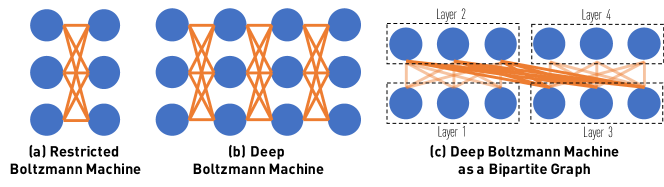
Figure 1. Restricted Boltzmann machines and deep Boltzmann machines as bipartite systems.

Markov chain Monte Carlo is a common approach to perform inference for RBMs, which involves sampling a configuration from the Gibbs distribution $\pi$. The de facto algorithm for this task is Gibbs sampling, in which the conditional probability of each step can be calculated from only the Hamiltonian. In this context, the alternating-scan algorithm we study corresponds to a layerwise scan — first update all variables in $V_{1}$ and then all variables in $V_{2}$. This scan order allows one to use efficient linear algebra primitives such as dense matrix multiplication implemented with GPUs or SIMD instructions on modern CPUs.

Deep Boltzmann Machines (DBM), introduced by Salakhutdinov and Hinton (2009), is a Deep Learning model that extends RBM to multiple layers as illustrated in Figure 1(b). This layer structure is indeed bipartite, shown in Figure 1(c). The scan order induced is thus to update odd layers first and even ones after. Like most deep learning models, the scan (evaluation) order of variables has significant impact on the speed and performance of the system. The layerwise implementation is particularly advantageous thanks to dense linear algebra primitives.

Given an RBM or DBM with $n$ variables, it is easy to see that $\log\pi_{\min}^{-1}$ is $O(n)$. Thus, Corollary 10 implies that, comparing to the random-update algorithm, the layerwise systematic scan algorithm incurs at most a $O(n^{2})$ slowdown in the convergence rate. This comparison result improves exponentially (in the worst case) upon previous result (He et al., 2016).

6. Experiments

Empirically evaluating the mixing time of Markov chains is notoriously difficult. In general, it is hard under certain complexity assumptions (Bhatnagar et al., 2011) and lower bounds have been established for more concrete settings by Hsu et al. (2015) (see also (Hsu et al., 2015) for a comprehensive survey on this topic). We evaluate the mixing time in either exact and straightforward or approximate but tractable ways, including (1) calculating directly using the transition matrix for small graphs, (2) taking advantage of symmetries in the state space for medium-sized graphs, and (3) using the coupling time (defined later) as a proxy of the mixing time for large graphs.

Mixing Time on Small Graphs. We evaluate the mixing time in a brutal force way, namely, we multiply the transition matrix until the total variation distance to the stationary distribution is below the threshold. Since the state space is exponentially large, such a method is only feasible in small graphs.

Figure 2 and Figure 3 contains the comparison of the mixing time for small graphs (RBMs of up to 12 variables and DBMs with 4 layers and 3 variable per layer). We vary (1) number of variables, (2) factor functions (shown as the entries of truth table in the caption), or (3) the weight of factors, in different figures and report the mixing times of random updates and layerwise scan. All solid lines count mixing time in # variable updates and the dotted line in # epochs.

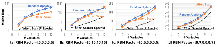
Figure 2. Mixing time of Gibbs samplers on Restricted Boltzmann Machines. See Section 6.

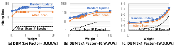
Figure 3. Mixing time of Gibbs samplers on Deep Boltzmann Machines. See Section 6.

We see that, empirically, alternating scan has comparable, sometimes better, mixing time than random updates, even when counting in the number of variable updates. On one hand, it confirms our result that the mixing time of alternating scan and random updates are similar. On the other, it shows that our result, although asymptotically tight for the worst case, is not “instance optimal”. This observation indicates promising future direction for beyond-worst case analysis.

Medium-sized Graphs. We now turn to Example 11, which has also been studied by He et al. (2016) and is asymptotically the worst case of Theorem 1. Due to certain symmetries, we have a much more succinct representation of the state space, and manage to calculate the mixing and relaxation times for mildly larger graphs (up to 50 variables). As illustrated in Figure 4, the alternating-scan sampler is slower than, but still comparable to the random-update sampler. This is consistent with the discussion in Example 11.

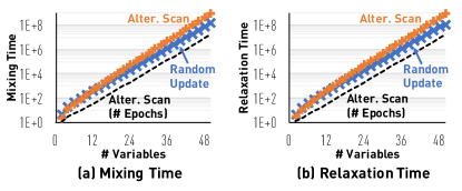
Figure 4. Mixing time comparison on medium-sized graphs.

Coupling Time on Large Graphs. Lastly, we use the coupling time as a proxy of the mixing time and estimate it on large graphs with $10^{4}$ variables and $5\times 10^{4}$ randomly chosen factors.

We use the grand coupling (Levin et al., 2009, Chapter 5). Let $T_{\sigma,\tau}$ be the first time two copies of the same Markov chain meet, with initial states $\sigma$ and $\tau$, under certain coupling. Then the coupling time is $\max_{(\sigma,\tau)\in\Omega^{2}}T_{\sigma,\tau}$. All of the models we tested are monotone (Peres and Winkler, 2013), in which the coupling time under the grand coupling can be easily evaluated by simulating from the top and bottom states. The coupling time is closely related to the mixing time (Levin et al., 2009, Chapter 5). In particular, it is an upper bound of the mixing time regardless of the coupling, and designing a good coupling is an important technique to prove rapid mixing (Bubley and Dyer, 1997). Our experimental findings are summarized in Figure 5.

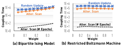
Figure 5. Coupling time comparison on large and random graphs.

In these experiments, we choose our parameters to stay within the rapidly mixing regime (Mossel and Sly, 2013) and avoid exponential mixing times. As we can see in Figure 5, alternating scan is faster than random updates (in terms of variable updates). Indeed, numerical evidence suggests that the speedup factor is close to $2$.

7. Concluding Remarks

In summary, we have shown that for a bipartite distribution, the relaxation time of the alternating-scan sampler (in terms of epochs) is no larger than that of the random-update sampler. This is asymptotically tight and implies a (weaker) comparison result on the mixing time. Future directions include more fine-grained comparison results, and going beyond bipartite distributions.

References

- Andrieu (2016) Christophe Andrieu. On random- and systematic-scan samplers. Biometrika, 103(3):719–726, 2016.
- Bhatnagar et al. (2011) Nayantara Bhatnagar, Andrej Bogdanov, and Elchanan Mossel. The computational complexity of estimating MCMC convergence time. In RANDOM, pages 424–435, 2011.
- Blanca et al. (2018) Antonio Blanca, Pietro Caputo, Alistair Sinclair, and Eric Vigoda. Spatial mixing and non-local Markov chains. SODA, 2018. To appear.
- Blei et al. (2003) David M. Blei, Andrew Y. Ng, and Michael I. Jordan. Latent Dirichlet allocation. J. Mach. Learn. Res., pages 993–1022, 2003.
- Bubley and Dyer (1997) Russ Bubley and Martin E. Dyer. Path coupling: A technique for proving rapid mixing in Markov chains. In FOCS, pages 223–231, 1997.
- Caracciolo et al. (1990) Sergio Caracciolo, Andrea Pelissetto, and Alan D. Sokal. Nonlocal Monte Carlo algorithm for self-avoiding walks with fixed endpoints. J. Stat. Phys., 60(1):1–53, Jul 1990.
- Diaconis and Ram (2000) Persi Diaconis and Arun Ram. Analysis of systematic scan Metropolis algorithms using Iwahori-Hecke algebra techniques. Michigan Math. J., 48(1):157–190, 2000.
- Diaconis and Saloff-Coste (1993) Persi Diaconis and Laurent Saloff-Coste. Comparison theorems for reversible Markov chains. Ann. Appl. Probab., 3(3):696–730, 08 1993.
- Dobrushin (1970) Roland L. Dobrushin. Prescribing a system of random variables by conditional distributions. Theory Probab. Appl., (3):458–486, 1970.
- Dyer et al. (2014) Martin Dyer, Catherine Greenhill, and Mario Ullrich. Structure and eigenvalues of heat-bath Markov chains. Linear Algebra Appl., 454:57 – 71, 2014.
- Dyer et al. (2006) Martin E. Dyer, Leslie Ann Goldberg, and Mark Jerrum. Systematic scan for sampling colourings. Ann. Appl. Probab., 16(1):185–230, 2006.
- Dyer et al. (2008) Martin E. Dyer, Leslie Ann Goldberg, and Mark Jerrum. Dobrushin conditions and systematic scan. Combin. Probab. Comput., 17(6):761–779, 2008.
- Fill (1991) James A. Fill. Eigenvalue bounds on convergence to stationary for nonreversible Markov chains, with an application to the exclusion process. Ann. Appl. Probab., 1(1):62–87, 1991.
- Gürbüzbalaban et al. (2017) Mert Gürbüzbalaban, Asu Ozdaglar, and Pablo Parrilo. Convergence rate of incremental aggregated gradient algorithms. SIAM J. Optimiz., 2017. To appear.
- Hastings (1970) Wilfred K. Hastings. Monte Carlo sampling methods using Markov chains and their applications. Biometrika, pages 97–109, 1970.
- Hayes (2006) Thomas P. Hayes. A simple condition implying rapid mixing of single-site dynamics on spin systems. In FOCS, pages 39–46, 2006.
- He et al. (2016) Bryan D. He, Christopher De Sa, Ioannis Mitliagkas, and Christopher Ré. Scan order in Gibbs sampling: Models in which it matters and bounds on how much. In NIPS, pages 1–9, 2016.
- Hsu et al. (2015) Daniel J. Hsu, Aryeh Kontorovich, and Csaba Szepesvári. Mixing time estimation in reversible Markov chains from a single sample path. In NIPS, pages 1459–1467, 2015.
- Jerrum (2003) Mark Jerrum. Counting, Sampling and Integrating: Algorithms and Complexity. Lectures in Mathematics, ETH Zürich. Birkhäuser, 2003.
- Jerrum and Sinclair (1993) Mark Jerrum and Alistair Sinclair. Polynomial-time approximation algorithms for the Ising model. SIAM J. Comput., 22(5):1087–1116, 1993. ISSN 0097-5397.
- Lafferty et al. (2001) John D. Lafferty, Andrew McCallum, and Fernando C. N. Pereira. Conditional random fields: Probabilistic models for segmenting and labeling sequence data. In ICML, pages 282–289, 2001.
- Lawler and Sokal (1988) Gregory F. Lawler and Alan D. Sokal. Bounds on the spectrum for Markov chains and markov processes: A generalization of Cheeger’s inequality. Trans. Amer. Math. Soc., 309(2):557–580, 1988.
- Levin et al. (2009) David A. Levin, Yuval Peres, and Elizabeth L. Wilmer. Markov chains and mixing times. American Mathematical Society, Providence, RI, 2009.
- Li (2009) Stan Z. Li. Markov Random Field Modeling in Image Analysis. 2009.
- Liu et al. (1995) Jun S. Liu, Wing H. Wong, and Augustine Kong. Covariance structure and convergence rate of the Gibbs sampler with various scans. J. Royal Stat. Soc. B, 57(1):157–169, 1995.
- Maire et al. (2014) Florian Maire, Randal Douc, and Jimmy Olsson. Comparison of asymptotic variances of inhomogeneous Markov chains with application to Markov chain Monte Carlo methods. Ann. Stat., 42(4):1483–1510, 08 2014.
- Mossel and Sly (2013) Elchanan Mossel and Allan Sly. Exact thresholds for Ising-Gibbs samplers on general graphs. Ann. Probab., 41(1):294–328, 2013.
- Peres and Winkler (2013) Yuval Peres and Peter Winkler. Can extra updates delay mixing? Comm. Math. Phys., 323(3):1007–1016, 2013.
- Peskun (1973) Peter H. Peskun. Optimum Monte-Carlo sampling using Markov chains. Biometrika, 60(3):607–612, 1973.
- Recht and Ré (2012) Benjamin Recht and Christopher Ré. Toward a noncommutative arithmetic-geometric mean inequality: Conjectures, case-studies, and consequences. In COLT, pages 11.1–11.24, 2012.
- Roberts and Rosenthal (1997) Gareth O. Roberts and Jeffrey S. Rosenthal. Geometric ergodicity and hybrid Markov chains. Electron. Commun. Probab., 2:13–25, 1997.
- Roberts and Rosenthal (2015) Gareth O. Roberts and Jeffrey S. Rosenthal. Surprising convergence properties of some simple Gibbs samplers under various scans. Int. J. Stat. Probab., 5(1), 2015.
- Roberts and Sahu (1997) Gareth O. Roberts and Sujit K. Sahu. Updating schemes, correlation structure, blocking and parameterization for the gibbs sampler. J. Royal Stat. Soc. B, 59(2):291–317, 1997.
- Rudolf and Ullrich (2013) Daniel Rudolf and Mario Ullrich. Positivity of hit-and-run and related algorithms. Electron. Commun. Probab., 18:49.1–49.8, 2013.
- Salakhutdinov and Hinton (2009) Ruslan Salakhutdinov and Geoffrey Hinton. Deep boltzmann machines. In AISTATS, pages 448–455, 2009.
- Shamir (2016) Ohad Shamir. Without-replacement sampling for stochastic gradient methods. In NIPS, pages 46–54, 2016.
- Sinclair (1992) Alistair Sinclair. Improved bounds for mixing rates of Markov chains and multicommodity flow. Comb. Probab. Comp., 1:351–370, 1992.
- Smolensky (1986) Paul Smolensky. Parallel distributed processing: Explorations in the microstructure of cognition. Information Processing in Dynamical Systems: Foundations of Harmony Theory, pages 194–281, 1986.
- Tierney (1998) Luke Tierney. A note on Metropolis-Hastings kernels for general state spaces. Ann. Appl. Probab., 8(1):1–9, 1998.
- Tosh (2016) Christopher Tosh. Mixing rates for the alternating Gibbs sampler over restricted Boltzmann machines and friends. In ICML, pages 840–849, 2016.
- Ullrich (2014) Mario Ullrich. Rapid mixing of Swendsen-Wang dynamics in two dimensions. Dissertationes Mathematicae, 502, 2014.