Covariant variational approach to Yang-Mills Theory: Thermodynamics

Abstract

The thermodynamics of $SU(2)$ Yang-Mills theory in the covariant variational approach is studied by relating the free action density in the background of a non-trivial Polyakov loop to the pressure of the gluon plasma. The correct subtraction of the vacuum contribution in the free action density is argued for. The Poisson resummed expression for the pressure can be evaluated analytically in limiting cases, and shows the correct Stefan-Boltzmann limit at $T\to\infty$, while the limit $T\to 0$ is afflicted by artifacts due to massless modes in the confined phase. Several remedies to remove these artifacts are discussed. Using the numerical $T=0$ solutions for the ghost and gluon propagators in the covariant variational approach as input, the pressure, energy density and interaction strength are calculated and compared to lattice data.

I Introduction

The low energy sector of quantum chromodynamics (QCD) and, in particular, its phase diagram are among the most actively researched topics in elementary particle physics. While heavy ion collisions at the large hadron collider (LHC) now begin to explore in detail the quark-gluon plasma at large temperatures and net baryon densities, the theoretical description of the full phase diagram through lattice simulations is still hampered by the sign problem. Alternative continuum methods are therefore of particular interest.

Among the most powerful continuum techniques are the so-called functional methods which, in one way or the other, amount to a closed set of integral equations connecting the low-order Green’s functions of the theory. For instance, the Dyson-Schwinger equations (DSE) are merely the equations of motion for the Green’s functions in momentum space, truncated by arbitrary (or educated) assumptions about higher vertices Fischer (2006); Alkofer and von Smekal (2001); Binosi and Papavassiliou (2009). Alternatively, one- or two-loop quantum corrections about non-perturbative extensions of the usual Faddeev-Popov (FP) action by mass terms Tissier and Wschebor (2010); *Tissier:2011ey or the Gribov-Zwanziger term Zwanziger (1989); *Zwanziger:1992qr have also been discussed Canfora et al. (2015). A more elaborated technique are the functional renormalization group (FRG) flow equations Pawlowski (2007); Gies (2012) which describe the behaviour of the relevant operators in the effective action as the theory evolves from the cutoff scale towards its infrared fixed point. Finally, if we are willing to dispense with manifest covariance, a particularly appealing and physically transparent picture emerges in the Hamiltonian approach to QCD in Coulomb gauge using variational techniques Feuchter and Reinhardt (2004); Reinhardt and Feuchter (2005); Epple et al. (2007).

Recently, we have added an alternative continuum approach to the list Quandt et al. (2014); Quandt and Reinhardt (2015, 2016) which attempts to combine the insightfulness of the Hamiltonian approach with the simplicity of a manifestly covariant setup. The method is based on Ansätze for the euclidean path integral measure, and results in a closed set of integral equations that can be conventionally renormalized. The numerical solutions give excellent agreement with zero-temperature lattice propagators Quandt et al. (2014), and also offer a satisfying description of the finite-temperature corrections, which agree with expectations from the lattice in all qualitative aspects Quandt and Reinhardt (2015). Recently, the method has also been used to study the deconfinement phase transition where it predicts the correct order of the transition for the colour groups $SU(2)$ and $SU(3)$ and gives quantitative values for the transition temperature which are in fair agreement with lattice data Quandt and Reinhardt (2016).

In the present paper, we want to complete the study of the Yang-Mills (YM) thermodynamics by computing its equation of state. The covariant variational approach is particularly well suited for this investigation, since it gives direct access to the free action density (and hence the pressure) of the gluon plasma. This is much more complicated in some of the functional methods mentioned above which only give (partial) information on the derivatives of the effective action. Nontheless, the equation of state has been computed in a variety of functional methods before: in the DSE approach, for instance, the phase structure of full QCD including quarks has been explored, both at finite temperature and finite density Fischer et al. (2011); Fischer and Luecker (2013). The pressure in pure Yang-Mills theory has also been calculated using massive extensions of the Faddeev-Popov action Reinosa et al. (2015, 2016), where comparison with lattice data gives a decent agreement in the deconfined phase, but deviations in the confined phase. In an alternative approach, the poor convergence of the perturbation series in the deconfined phase can be stabilized by non-perturbative resummation techniques Fukushima and Su (2013), which yield a good description of the pressure in this region, but lack e.g. the peak structure in the interaction strength. Finally, the pressure has also been computed using continuum methods in Coulomb gauge. A first approach using the Gribov formula as the temperature-independent dispersion relation for a gas of free gluon excitations gave results comparable to massive free particles while lacking a true phase transition Zwanziger (2005). In Ref. Reinhardt and Heffner (2017a), good agreement with lattice data could be achieved within the variational Hamiltonian approach, provided that the grand canonical density operator was constructed from a full ensemble of approximate thermal states above the vacuum. In an alternative Hamiltonian formulation, the thermodynamics can also be related to the ground state properties of YM-theory on a semi-compactified space manifold $\mathbb{R}^{2}\times S^{1}$ Reinhardt (2016). In this case, the pressure exhibits significant deviations from the expected behaviour Reinhardt and Heffner (2017b). This can be traced to the violation of $O(4)$ invariance underlying the spatial compactification.

This paper is organised as follows: In the next section, we review the covariant variation principle and show how the free energy can naturally be accessed within this approach. Section III summarizes the previous results obtained for YM theory and, in particular, the computational technique for the Polyakov loop study Quandt and Reinhardt (2016), which will also be used (with appropriate modifications) for the present investigation. The necessary background field technique is described in more detail in section IV, where we also discuss the correct subtraction of the vacuum energy and the analytical limits of our solution. Section V presents our numerical results for the various thermodynamical quantities in comparison to lattice data. In the last sub-section V.3, we discusses the origin of deviations and artifacts in the confined region, and speculate about possible remedies. We conclude the manuscript with a brief summary and an outlook on future investigations within the present approach.

II Thermodynamics and the variation principle

Let us briefly recall the variation principle for the effective action of pure Yang-Mills theory in Euclidean spacetime. The variation is with respect to the normalized path integral measure $d\mu(A)$ which is used to compute expectation values of arbitrary observables built from the gauge field $A\equiv A_{\mu}^{a}(x)$. Within the space of such probability measures, quantum field theory singles out the particular Gibb’s type of measure

$$d\mu_{0}[A]=Z^{-1}\cdot\mathcal{D}A\,\mathcal{J}[A]\,\exp\Big{\{}-\hbar^{-1}\,S_{\rm fix}[A]\Big{\}}\,,$$ (1)

where $S_{\rm fix}=S_{\rm YM}+S_{\rm gf}$ is the classical euclidean action including the gauge-fixing term, and $\mathcal{J}[A]$ is the corresponding Faddeev-Popov (FP) determinant. (We do not need to specify the gauge condition at this point.) The partition function

$$Z\equiv\int\mathcal{D}A\,\mathcal{J}[A]\,\exp\Big{\{}-\hbar^{-1}\,S_{\rm fix}[A]\Big{\}}$$ (2)

is required for normalization. Although it is formally a gauge-dependent quantity, the Faddeev-Popov procedure, or Becchi-Rouet-Stora-Tyutin (BRST) symmetry, entails that $Z$ agrees in all local gauges. The moments of the Gibbs-measure $d\mu_{0}$ from eq. (1) are the usual Schwinger functions of euclidean field theory. Moreover, Gibb’s measure minimizes the free action

$$F(\mu)\equiv\big{\langle}\,S_{\rm fix}\,\big{\rangle}_{\mu}-\hbar\,\mathcal{W}(\mu)$$ (3)

where the relative entropy

$$\mathcal{W}(\mu)=-\left\langle\,\ln(\rho/\mathcal{J})\,\right\rangle_{\mu}\,.$$ (4)

describes the available phase space for quantum fluctuations in the trial measure $d\mu\equiv\mathcal{D}A\,\rho[A]$ relative to the FP determinant, which is the natural measure on the gauge orbit. Moreover, the absolute minimum of the free action is given by

$$\min_{\mu}\,F(\mu)=F(\mu_{0})=-\ln Z\,,$$ (5)

which is hence also a gauge-invariant quantity. It is convenient to perform the minimization of the free action in two steps, by first constraining $F(\mu)$ such that the expectation value of an arbitrary operator $\Omega[A]$ is fixed at a prescribed classical value $\omega$. The minimum is then called the effective action for the operator $\Omega$,

$$\Gamma[\omega]=\min_{\mu}\,\Big{\{}F(\mu)\,\big{|}\,\langle\,\Omega\,\rangle_{\mu}=\omega\Big{\}}\,.$$ (6)

The most common choice is to take $\Omega[A]$ as the quantum gauge field itself (with classical value $\langle A\rangle_{\mu}=\mathscr{A}$) whence the derivatives of $\Gamma[\mathscr{A}]$ become the proper functions of the full quantum theory. The FP procedure will only ensure that $\Gamma[\omega]$ is gauge invariant, if $\Omega$ happens to be a gauge-invariant operator; in particular, the effective action $\Gamma[\mathscr{A}]$ is a gauge-dependent functional, and so are the proper functions. However, the absolute minimum of $\Gamma[\mathscr{A}]$ is related to the free energy by

$$\min_{\mathscr{A}}\,\Gamma[\mathscr{A}]=F(\mu_{0})=-\ln Z$$ (7)

and must hence agree in all gauges, provided that no approximations have been made.

To study the thermodynamics of the system, we can introduce finite temperature using the imaginary time formalism, i.e. we compactify the Euclidean time direction to the finite interval $[0,\beta]$ and impose periodic boundary conditions in this direction for both the gluons and the ghosts Bernard (1974). This will make all quantities introduced above depend on the inverse temperature $\beta$. In particular, the minimum of the free action can now be written

$$\min_{\mu}F_{\beta}(\mu)=\min_{\mathscr{A}}\Gamma_{\beta}[\mathscr{A}]=-\ln Z(\beta)\equiv V_{3}\,\beta\cdot f(\beta,V_{3})\,,$$ (8)

where $V_{3}$ is the spatial volume. In gauges which do not break the residual spatial $O(3)$ symmetry explicitly, the density $f$ depends on $V_{3}$ only through the spatial boundary conditions, which are expected to become immaterial in the infinite volume limit, i.e. the quantity

$$f(\beta)\equiv\lim_{V_{3}\to\infty}f(\beta,V_{3})$$

should exist for such gauges and, by gauge invariance of $Z$, eventually also in all other local gauges. Other thermodynamical quantities can be deduced directly from $f(\beta)$: in a grand canonical ensemble, the chemical potential for the (massless) gluons must vanish and we have the relations listed in the following table:

pressure	$\quad p(\beta)=-f(\beta)$
energy density	$\quad\epsilon(\beta)=f+\beta\,\partial f/\partial\beta$
entropy density	$\quad w(\beta)=\beta(\epsilon+p)=\beta^{2}\,\partial f/\partial\beta$
interaction strength	$\quad\Delta(\beta)=\beta^{4}(\epsilon-3p)=-\beta\,\partial(p\beta^{4})/\partial\beta$

The interaction strength measures the deviation from the ideal gas limit, since $p\sim T^{4}$ and hence $\Delta=0$ for an ultra-relativistic gas at vanishing chemical potential. The only independent thermodynamical information about the gluon plasma is thus contained in the equation of state, i.e. the pressure function $p(\beta)$, which is the main target of the present investigation.

III The variational approach

So far, all considerations apply to the exact minimum of the free action eq. (3) attained for the Gibbs measure eq. (1), or, equivalently, for the exact minimum of the effective action (6). The variational method restricts the space of trial measures $d\mu$ to some subset of normalized measures for which (i) the constraint $\langle\Omega\rangle_{\mu}=\omega$ can be implemented conveniently, and (ii) the relevant expectation values can be evaluated reliably.

As a first step, we have to fix a gauge. At zero temperature, the unbroken spacetime $O(4)$ invariance entails that the most natural choice is Landau gauge. This is not because the effective action $\Gamma[\mathscr{A}]$ would be particularly easy to calculate in this gauge — it is, in fact, a very hard calculation for classical fields $\mathscr{A}_{\mu}^{a}$ that have arbitrary colour and Lorentz orientation Quandt et al. (2014). The real reason for using Landau gauge is that the manifestly unbroken spacetime $O(4)$ invariance entails $\langle A_{\mu}\rangle=0$, i.e. the effective action must take its minimum at the classical field $\mathscr{A}_{\mu}=0$. This allows us to concentrate the variational search eq. (6) to measures with vanishing first moment $\langle A\rangle_{\mu}=0$, which simplifies the calculation considerably.

In Refs. Quandt et al. (2014); Quandt and Reinhardt (2015), we have thus made a simple yet physically sensible ansatz and considered only Gaussian measures of the form

$$d\mu[A]=\mathcal{N}\cdot\mathcal{D}A\,\mathcal{J}[A]^{1-2\alpha}\cdot\exp\Bigg{\{}-\frac{1}{2}\int d(x,y)\,A_{\mu}^{a}(x)\,\omega_{\mu\nu}^{ab}(x,y)\,A^{b}_{\nu}(y)\Bigg{\}}\,,$$ (9)

where the constant $\alpha$ and the kernel $\omega$ are variational parameters. Physically, the picture conveyed by this ansatz is that of a weakly interacting (constituent) gluon with a enhanced weight (for $\alpha>0$) near the Gribov horizon. If the FP determinant

$$\mathcal{J}[A]=\frac{\mathrm{det}\big{(}-\partial_{\mu}\hat{D}_{\mu}\big{)}}{\mathrm{det}(-\partial^{2})}\,.$$ (10)

is treated to the same formal loop order as the remaining exponent in eq. (9), it can be replaced by the simpler expression

$$\ln\mathcal{J}[A]\approx-\frac{1}{2}\,\int d(x,y)\,A_{\mu}^{a}(x)\,\chi^{ab}_{\mu\nu}(x,y)\,A_{\nu}^{b}(y)\,,$$ (11)

where the curvature $\chi$ can be expressed through the Faddeev-Popov ghost operator $G=(\partial_{\mu}\hat{D}^{\mu})^{-1}$ and the bare ($\Gamma_{0}$) and full ($\Gamma$) ghost-gluon vertex,

$$\chi^{ab}_{\mu\nu}(x,y)=-\left\langle\frac{\delta^{2}\ln\mathcal{J}}{\delta A_{\mu}^{a}(x)\,\delta A_{\nu}^{b}(y)}\right\rangle=-\mathrm{Tr}\Big{[}\,\langle G\rangle\,\Gamma_{\mu}^{a}(x)\,\langle G\rangle\,\Gamma_{0,\nu}^{b}(y)\,\Big{]}=\quad\begin{minipage}{85.35826pt}\includegraphics[width=85.35826pt]{curvature.pdf}\end{minipage}\,.$$ (12)

To the given loop order, the trial measure (9) becomes exactly Gaussian and the variation kernel only enters in the combination $\bar{\omega}=\omega+(1-2\alpha)\chi$, which equals the inverse gluon propagator. (The value of the variational parameters $\alpha$ is hence immaterial and, for simplicity, we write $\omega(k)$ instead of $\bar{\omega}(k)$ in the following.) The Gaussian is centered at $\langle A_{\mu}\rangle=0$ as explained above, and we can compute the effective action $\Gamma[\mathscr{A}=0;\omega]$ as a functional of the variational kernel $\omega$. Alternatively, we can view the kernel $\omega$ as the classical value of the inverse gluon propagator at $\mathscr{A}=0$, and interprete $\Gamma[\mathscr{A}=0;\omega]$ as its effective action. Either way, the gap equation $\delta\Gamma/\delta\omega=0$ leads to an integral equation for the kernel $\omega$, which can be renormalized and solved together with the resolvent identity for the ghost form factor

$$\eta(k)\equiv k^{2}\,\mathrm{tr}_{A}\,\langle G(k)\rangle$$ (13)

entering eq. (12). For further details, see Refs. Quandt et al. (2014); Quandt and Reinhardt (2016) and Fig. 1.

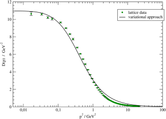
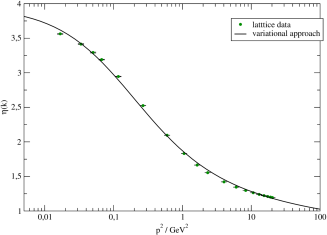
Figure 1: The zero-temperature gluon propagator (left) and the ghost form factor (right) for the decoupling type of solution, compared to high-precision lattice data Bogolubsky et al. (2009).

These considerations are no longer true at finite temperature. In this case, the $O(4)$ spacetime symmetry is manifestly broken since the heat bath singles out a rest frame. In the imaginary time formalism, the euclidean time interval is compactified to the interval $[0,\beta]$ with periodic boundary conditions for the gluons and ghosts Bernard (1974), and we have a residual spatial $O(3)$ symmetry only. This has various consequences:

1. Integrations over the momentum component $k_{0}$ are replaced by sums over Matsubara frequencies $k_{0}=2\pi n/\beta$ with $n\in\mathbb{Z}$,

   $$\int\frac{d^{4}k}{(2\pi)^{4}}\cdots\quad\Longrightarrow\quad\int_{\beta}\text{\dj}k\cdots\equiv\beta^{-1}\sum_{n\in\mathbb{Z}}\int\frac{d^{3}\mathbf{k}}{(2\pi)^{3}}\cdots$$

2. Tensors such as the kernel $\omega_{\mu\nu}^{ab}(k)$ or the curvature $\chi^{ab}_{\mu\nu}(k)$ can now be decomposed into two independent Lorentz structures which are both $4D$ transversal, but $3D$ longitudinal or perpendicular to the heat bath. The gap equation couples the corresponding scalar kernels $\omega_{\perp}(k_{0},|\mathbf{k}|)$ and $\omega_{\|}(k_{0},|\mathbf{k}|)$, as well as the ghost form factor $\eta(k_{0},|\mathbf{k}|)$ for all Matsubara frequencies $k_{0}=2\pi n/\beta$. The finite temperature system is thus easily several orders of magnitude more expensive than the $T=0$ calculation. For practical reasons, we could not include more than about $40$ Matsubara modes in Ref. Quandt and Reinhardt (2015), which was limiting the temperature to not much smaller than the critical temperature $T^{\ast}$. In this temperature range, the resulting propagators agree in all qualitative aspects with the lattice findings. In particular, there is a slight enhancement of the ghost form factor as compared to $T=0$ and a moderate suppression of the gluon propagators in the deep infra-red, with higher temperature sensitivity in the components longitudinal to the heat bath.

3. The classical field $\mathscr{A}$ which minimizes the effective action need no longer be vanishing. Global colour and spatial $O(3)$ invariance only entail that the minimizing $\mathscr{A}$ can have no spatial component, and the remaining temporal part $\mathscr{A}_{0}$ should be constant and colour diagonal. In fact, a minimizing classical field of this type can serve as an alternative order parameter for the deconfinement phase transition, since it obeys the so-called Polyakov gauge condition, $\partial_{0}\mathscr{A}_{0}=0$. The most convenient way to introduce a non-vanishing classical field of this type is through the background field formalism.

IV Background field formulation at finite temperature

Let us elaborate on the last point: in background gauge, we decompose the quantum field $A_{\mu}=\mathsf{a}_{\mu}+Q_{\mu}$, where $\mathsf{a}_{\mu}$ is the arbitrary background field, and subject the fluctuations to the gauge condition $[D_{\mu}(\mathsf{a}),Q_{\mu}]=0$, or

$$\hat{\mathsf{d}}_{\mu}^{ab}Q_{\mu}^{b}\equiv(\partial_{\mu}\delta^{ab}-f^{abc}\mathsf{a}_{\mu}^{c})\,Q_{\mu}^{b}=0\,.$$ (14)

Here and in the following, $\mathsf{d}_{\mu}\equiv D_{\mu}(\mathsf{a})=\partial_{\mu}+\mathsf{a}_{\mu}$ is the covariant derivative of the background field, and the hat over a symbol denotes the adjoint representation.

The effective action for the classical fluctuation field $\mathscr{Q}_{\mu}=\langle Q_{\mu}\rangle$ depends explicitly on the chosen background field, $\Gamma_{\mathsf{a}}[\mathscr{Q}]$. It is also easy to see that $\Gamma_{\mathsf{a}}[\mathscr{Q}]=\widetilde{\Gamma}_{\mathsf{a}}[\mathsf{a}+\mathscr{Q}]$, where $\widetilde{\Gamma}_{\mathsf{a}}[\mathscr{A}]$ is the usual effective action of the total classical field $\mathscr{A}_{\mu}$, subject to the background gauge condition $\hat{\mathsf{d}}_{\mu}\,(A_{\mu}-\mathsf{a}_{\mu})=0$. From the considerations in the previous chapter, we know that the minimum of $\widetilde{\Gamma}_{\mathsf{a}}[\mathscr{A}]$ at any temperature equals the gauge-invariant free action, and this minimum occurs at a constant temporal classical field $\mathscr{A}_{\mu}=\delta_{\mu 0}\,\mathscr{A}_{0}$, provided that the background field itself does not break the residual spatial $O(3)$ symmetry. To ensure this condition, it is then convenient to choose the background field itself in this special form, $\mathsf{a}_{\mu}=\mathsf{a}_{0}\,\delta_{\mu 0}$, and further set $\mathscr{Q}_{\mu}=0$. The minimum of $\widetilde{\Gamma}_{\mathsf{a}}[\mathsf{a}]$ for a constant, Abelian background field $\mathsf{a}_{0}$ then yields directly the gauge-invariant free action.

In Ref. Quandt and Reinhardt (2016), we have employed the interpretation of $\mathsf{a}_{0}$ as an alternative order parameter for the deconfinement phase transition Braun et al. (2010); Reinosa et al. (2016), and evaluated its effective potential within our approach. Technically, the transfer of the variational approach from Landau to background gauge is rather simple and amounts to the replacement of the partial derivative by its covariant counterpart, $\partial_{\mu}\to\hat{\mathsf{d}}_{\mu}$ in a few strategic places. Since the background field $\mathsf{a}_{0}$ is constant, the replacement corresponds to a mere shift in the momentum arguments and we can recycle the solution of the variational problem in Landau gauge with shifted arguments. More precisely, $\hat{\mathsf{d}}_{\mu}$ is a colour matrix in the adjoint representation and we must first go to a colour base in which $\hat{\mathsf{d}}_{\mu}$ is diagonal, $\hat{\mathsf{d}}_{\mu}^{ab}=\mathbf{e}^{a}_{\sigma}\,(\mathbf{e}^{b}_{\tau})^{\ast}\,\delta^{\sigma\tau}\,\mathsf{d}_{\mu}^{\sigma}$. This is the so-called root decomposition of the colour algebra, and the momentum shift becomes

$$\partial_{\mu}(p)=ip_{\mu}\,\,\,\to\,\,\,\mathsf{d}_{\mu}^{\sigma}(p)=i(p_{\mu}-\boldsymbol{\sigma}\mathsf{a}_{0}\,\delta_{\mu 0})\equiv ip_{\mu}^{\sigma}$$ (15)

for every simple root vector $\boldsymbol{\sigma}$. We must also replace the factor $(N^{2}-1)$ from the colour traces in Landau gauge by a sum over all simple roots.

It should be emphasized that this recipe only holds when using the $T=0$ kernels even at finite temperature. The temperature dependent kernels involve the background field in other ways than just through the covariant derivative $\mathsf{d}_{\mu}$, and the same also happens if we go beyond two-loop in the effective potential. However, as we have seen above, the kernels are only mildly affected by temperature, and it has been further argued in Ref. Braun et al. (2010) that the dominant contributions to the integral equations come from momentum and frequency regions where the finite temperature corrections to the kernels are negligible. We will thus base our calculations on the $T=0$ solutions $\{\omega(k),\eta(k)\}$ in Landau gauge, cf. Fig. 1.

In background gauge, we therefore replace the measure eq. (9) by a similar Gaussian Quandt and Reinhardt (2016) centered at $\langle A_{\mu}\rangle=\mathsf{a}_{0}\,\delta_{\mu 0}$ and $\langle Q_{\mu}\rangle=\mathscr{Q}_{\mu}=0$ as justified above,

$$d\mu =\mathcal{N}\cdot\mathcal{D}A\,\mathcal{J}(A)^{1-2\alpha}\,\exp\left[-\frac{1}{2}\,\int d(x,y)\,(A-\mathsf{a})^{a}_{\mu}\,\omega_{\mu\nu}^{ab}(x,y)\,(A-\mathsf{a})^{b}_{\nu}(y)\right]$$

$$=\mathcal{N}\cdot\mathcal{D}Q\,\mathcal{J}(\mathsf{a}+Q)^{1-2\alpha}\,\exp\left[-\frac{1}{2}\,\int d(x,y)\,Q^{a}_{\mu}(x)\,\omega_{\mu\nu}^{ab}(x,y)\,Q^{b}_{\nu}(y)\right]\,.$$ (16)

We can now follow the calculation as in the Landau gauge case: in the ghost sector, we have to apply the rainbow approximation stating that the full ghost-gluon vertex on the r.h.s. of the curvature (12) is bare. This simplification is expected to be very robust, since the ghost-gluon vertex is known to be non-renormalized in Landau gauge due to Taylor’s identity Taylor (1971), and lattice studies also indicate that it receives only very mild corrections in the infra-red Ilgenfritz et al. (2007); Sternbeck (2006). With this approximation, the curvature can be expressed solely in terms of the variational kernel $\omega(k)$ and the ghost form factor $\eta(k)$, for which a separate resolvent identity exists. The result is the free action and the gap equation in background gauge Quandt and Reinhardt (2016)

$$F[\mathsf{a}] =\frac{1}{2}\,\Big{[}\gamma(1,2)+\chi(1,2)+M_{0}^{2}(1,2)\Big{]}\,\omega^{-1}(1,2)+\frac{1}{2}\ln\det\omega+\frac{1}{2}\,\ln\det(-\hat{\mathsf{d}}^{2})-\ln\mathcal{J}[\mathsf{a}]\,,$$

$$\omega(1,2) =\gamma(1,2)+2\chi(1,2)+2M_{0}^{2}(1,2)-\chi_{0}\,.$$ (17)

To keep the formulas compact, we have used an obvious shorthand notation where a roman digit stands for the combination of spactime, Lorentz and adjoint color index, $1\equiv(x,\mu,a),\,\,2\equiv(y,\nu,b)$ etc., and repeated indices are summed or integrated over. In momentum space, $M_{0}^{2}$ and $\chi_{0}$ are (quadratically divergent) constants that must eventually be removed by renormalization. As layed out in detail in Refs. Quandt et al. (2014) and Quandt and Reinhardt (2016), we need three counter-terms

$$\mathcal{L}_{\rm CT}=\delta Z_{A}\cdot\frac{1}{4}\big{(}\partial_{\mu}A_{\nu}^{a}-\partial_{\nu}A_{\mu}^{a}\big{)}^{2}+\delta M^{2}\cdot\frac{1}{2}\big{(}A_{\mu}^{a}\big{)}^{2}+\delta Z_{c}\cdot\big{(}\partial_{\mu}\eta\big{)}^{2}\,.$$ (18)

To fix the coefficients, we prescribe the values $Z$ and $M_{A}$ in the conditions $\omega(\mu_{0})=ZM_{A}^{2}$ and $\omega(\mu)=Z\mu^{2}$ at two different scales $\mu_{0}\ll\mu$. This removes all quadratic and subleading logarithmic divergences from the gap equation. In addition, we must also remove the logarithmic divergence in the ghost equation, for which we fix of the ghost form factor $\eta(\mu_{c})\equiv\eta_{0}$ at $\mu_{c}\to 0$. The reasoning here is that the present approach allows not only for a single solution, but instead for a whole family of scaling and decoupling solutions, which differ only in their deep infrared behaviour Quandt et al. (2014). Fixing the ghost form factor at a small scale thus selects a specific type of solution and avoids numerical instabilities in the deep infrared.

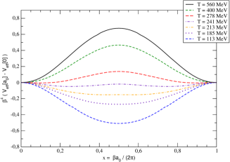
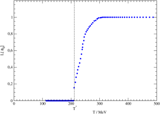
Figure 2: Left: The effective potential $V_{\rm eff}(x)$ for the Polyakov loop on the $SU(2)$ Weyl alcove $x\in[0,1]$ defined in eq. (21). Right: The Polyakov Loop as a function of temperature, extracted from the minimum of $V_{\rm eff}$.

After renormalization, the mass and wave function counter-terms for the gluon render the curvature finite, $\chi(k)-\chi_{0}\to\chi_{R}(k)$, and the gap equation becomes

$$\omega(1,2)=Z\,\gamma(1,2)+2\chi_{R}(1,2)\,.$$ (19)

If we insert this solution into the free action (with the counter term contribution added), we obtain the renormalized effective action of the background field in the general form

$$\Gamma[\mathsf{a}]=-\frac{1}{2}\,\chi_{R}(1,2)\,\omega^{-1}(1,2)+\frac{1}{2}\ln\det\omega+\frac{1}{2}\,\ln\det(-\hat{\mathsf{d}}^{2})-\ln\mathcal{J}[\mathsf{a}]\,.$$ (20)

The kernels $\omega(k)$ and $\chi_{R}(k)$ are the same functions as computed from the Landau gauge system (cf. Fig. 1), but with the momentum argument $k$ shifted by the background field in the colour direction of the root vectors, cf. eq. (15). For $G=SU(2)$, there is only a single Cartan generator $T^{3}=\sigma^{3}/(2i)$ and hence a single positive root, and the fundamental domain (Weyl alcove) for the background $\mathsf{a}_{0}$ is conveniently parametrized by the dimensionless quantity

$$x\equiv\beta\mathsf{a}_{0}^{3}/2\pi\in[0,1]\,.$$ (21)

Center symmetry acts as $x\to 1-x$ on these coordinates, and the center symmetric point is hence located at $x=1/2$. At this point, the Polyakov loop $\mathsf{P}$ vanishes and we have confinement, while the maximally center breaking configurations with $\mathsf{P}=1$ located at $x=0$ and $x=1$ describe deconfinement. The deconfinement phase transition thus occurs as a rapid change of the location of the minimum of the effective potential $V_{\rm eff}(x)$, from $x=0$ and $x=1$ at $T>T^{\ast}$ to $x=1/2$ at $T\leq T^{\ast}$. This is shown in Fig. 2. The transition is clearly second order for $G=SU(2)$ and the phase transition temperature can be translated into absolute units by using the mass scale $M_{A}^{2}$ introduced in the $T=0$ propagators. This gives a value of $T^{\ast}\approx 214\,\mathrm{MeV}$ which is in fair agreement with the lattice findings of $T^{\ast}\approx 300\,\mathrm{MeV}$ Lucini et al. (2004), in particular since the determination of the scale $M_{A}^{2}$ from the fit of the variational solutions to lattice data has rather large uncertainties.

Returning to eq. (20), we can use the curvature representation of the FP determinant to the given loop order, go to Fourier space and work out the colour traces using the root decomposition, cf. eq. (15). After introducing spherical coordinates for the remaining spatial loop integral, the angles can be integrated out explicitly and we obtain

$$\beta^{4}\,f_{\beta}(x) =4\pi\int_{0}^{\infty}dq\,q^{2}\,\sum_{n\in\mathbb{Z}}\,\Bigg{[}\phi(k_{n}(x))+\frac{1}{2}\,\phi(k_{n}(0))\Bigg{]}$$ (22)

Here, $q\equiv|\mathbf{k}|\beta/(2\pi)$ is the rescaled dimensionless momentum norm and

$$k_{n}(x)\equiv\frac{2\pi}{\beta}\sqrt{(n+x)^{2}+q^{2}}\,.$$ (23)

The integrand in eq. (22) is given explicitly by

$$\phi(k)\equiv 3\,\ln\omega(k)-3\,\frac{\chi_{R}(k)}{\omega(k)}-\ln\,k^{2}\,.$$ (24)

This quantity contains the dispersion relations of all particle fluctuations in our Gaussian ansatz: we have three non-perturbative transversal gluon modes with dispersion $\omega(k)$, the curvature which measures the deviation of the non-perturbative ghosts from the free ghosts, and the combination of these two perturbative ghost modes with the one longitudinal gluon, which share the same free dispersion relation $\omega(k)=k^{2}$.

In principle, the (negative) minimum of eq. (22) gives the pressure at inverse temperature $\beta$, which is our primary goal. However, eq. (22) is neither in a form suitable for numerical evaluation, nor is it finite to start with, even though we have added all available counter terms. The reason for this divergence is that eq. (22) still contains the unobservable energy of the vacuum, which must be subtracted. In the present case, this subtraction becomes particularly transparent if we Poisson resum the Matsubara series in eq. (22),

$$f_{\beta}(x)=\frac{4\pi}{\beta^{4}}\,\int_{0}^{\infty}dq\,q^{2}\,\int_{-\infty}^{\infty}dz\,\sum_{\nu\in\mathbb{Z}}e^{2\pi i\nu z}\,\Bigg{[}\phi\left(\frac{2\pi}{\beta}\,\sqrt{(z+x)^{2}+q^{2}}\right)+\frac{1}{2}\,\phi\left(\frac{2\pi}{\beta}\,\sqrt{z^{2}+q^{2}}\right)\Bigg{]}\,.$$ (25)

The vacuum energy is precisely the $\nu=0$ contribution to the Poisson sum, which must hence be omitted to effect the proper subtraction $\delta f$. To see this, we can take the $\nu=0$ contribution, shift $z\to z-x$ in the inner integral and change variables $s=z/\beta$ and $p=q/\beta$,

$$\delta f=6\pi\,\int_{0}^{\infty}dp\,p^{2}\int_{-\infty}^{\infty}ds\,\phi\big{(}2\pi\,\sqrt{s^{2}+p^{2}}\big{)}\,.$$ (26)

As can be seen, $\delta f$ is a constant contribution to the free action density independent of the background field $x$ and of temperature $\beta$. This (divergent) contribution is present in the free energy density $f_{\beta}(x)$ at any temperature and any background, and can hence be identified with the constant vacuum energy density or cosmological constant.

After omitting the $\nu=0$ contribution in eq. (25), we can further evaluate the free energy density using the same analytical techniques that have have also been used for the effective action of the Polyakov loop in Ref. Quandt and Reinhardt (2016). For completeness, we have summarized this evaluation in appendix A; the result is the simple expression

$$u(x,\beta)\equiv\beta^{4}\,f_{\beta}(x)=-\frac{2}{\pi^{2}}\,\sum_{\nu=1}^{\infty}\frac{\cos(2\pi\nu x)+\frac{1}{2}}{\nu^{4}}\,h(\beta\nu)\,.$$ (27)

Here, the function $h(\lambda)$ is the Hankel transform of the dispersion $\phi(k)$ from eq. (24),

$$h(\lambda)\equiv-\frac{\lambda^{3}}{4}\,\int_{0}^{\infty}dk\,k^{2}\,J_{1}(\lambda k)\,\phi(k)\,.$$ (28)

As it stands, this transformation is guaranteed to exist for integrands $\phi(k)$ which are regular at the origin and vanish sufficiently fast at $k\to\infty$, for instance as $\mathcal{O}(k^{-\frac{5}{2}})$. However, we need to extend this domain to a larger class of functions $\phi(k)$ with a weaker decay, or even a mild (logarithmic) divergence at $k\to\infty$, cf. eq. (24). To this end, we integrate by parts twice and obtain

$$h(\lambda)=\frac{1}{4}\,\int_{0}^{\infty}dk\,\Big{[}2J_{0}(\lambda k)-k\lambda J_{1}(\lambda k)\Big{]}\,\big{[}\phi^{\prime}(k)+k\phi^{\prime\prime}(k)\big{]}\,.$$ (29)

This formula has a much larger domain of convergence and is well suited for numerical evaluation, even when $\phi(k)$ diverges (mildly) at large $k$. The discarding of the boundary terms can be justified by distributional arguments, cf. appendix B. As a further test, we have also considered a free boson of mass $m$, where eq. (29) gives the expected result (see also appendix C),

$$h(\lambda)=\frac{1}{2}\,(\lambda m)^{2}\,K_{2}(\lambda m)\,.$$ (30)

Eqs. (27) and (29) are the main formulas used for our numerical study in the next section. Before presenting these results, let us first discuss some analytical properties and limits of our approach.

In eq. (27), the argument of the Hankel transform is $\lambda=\beta\nu$, i.e. the zero temperature limit involves $h_{\infty}\equiv\lim\limits_{\lambda\to\infty}h(\lambda)$. This limit is, however, non-uniform with respect to the particle mass. To see this, consider the simple case of a free boson of mass $m$ discussed in appendix C. For any non-vanishing mass $m>0$, we obtain the limit $h_{\infty}=0$, while taking $m\to 0$ first yields $h(\lambda)=1$ for all $\lambda$, and in particular $h_{\infty}=1$. This means that only massless modes contribute, at very small temperatures, to the rhs of eq. (27). Conversely, the high temperature limit $\beta\to 0$ is uniform, since $h(0)=1$ for all free bosonic modes, irrespective of their mass.

This observation allows us to easily deduce the high and low temperature limit of the rescaled free energy $u(x,\beta)$ from eq. (27): As we have seen above, every free massless boson mode is characterized by $h(\beta\nu)=1$ at any temperature, which from eq. (27) gives the contribution

$$-\frac{2}{\pi^{2}}\sum_{\nu=1}^{\infty}\frac{\cos(2\pi\nu x)+\frac{1}{2}}{\nu^{4}}=\frac{2}{3}\,\pi^{2}x^{2}\,(1-x)^{2}-\frac{\pi^{2}}{30}$$ (31)

to $u(x,\beta)$. Massive free boson modes give the same contribution at high energies, while they do not contribute to $u(x,\beta)$ at small temperatures $\beta\to\infty$. The proper limit is now a matter of counting degrees of freedom: the only massless degrees of freedom at small temperatures are the longitudinal gluon and the two ghost degrees of freedom. Together, these represent $(-2)+1=-1$ free massless bosonic degree of freedom (ghost dominance) and we have

$$u_{\infty}(x)\equiv\lim_{\beta\to\infty}\beta^{4}\,f_{\beta}(x)=-\frac{2}{\pi^{2}}\sum_{\nu=1}^{\infty}\frac{\cos(2\pi\nu x)+\frac{1}{2}}{\nu^{4}}\cdot(-1)=-\frac{2}{3}\,\pi^{2}x^{2}(1-x)^{2}+\frac{\pi^{2}}{30}\,.$$ (32)

Conversely, all dispersion relations become free at sufficiently high temperatures, and we expect the usual 4 massless gluon degrees of freedom, partially cancelled by the two free ghost degrees of freedom, for a total of $(+2)$ massless bosonic modes. This gives the limit

$$u_{0}(x)\equiv\lim_{\beta\to 0}\beta^{4}\,f_{\beta}(x)=-\frac{2}{\pi^{2}}\sum_{\nu=1}^{\infty}\frac{\cos(2\pi\nu x)+\frac{1}{2}}{\nu^{4}}\cdot(+2)=+\frac{4}{3}\,\pi^{2}x^{2}(1-x)^{2}-\frac{\pi^{2}}{15}\,.$$ (33)

The limits (32) and (33) will also be confirmed by the numerical study in the next section.

The pressure is the negative minimum of the free energy density with respect to the background field $x$. For high temperatures, this minimum is reached at $x=0$ (deconfinement) so that

$$\lim_{T\to\infty}\frac{p(T)}{T^{4}}=\frac{\pi^{2}}{15}\,,$$ (34)

which is the correct Stefan-Boltzmann limit for the colour group $G=SU(2)$. At very small temperatures, by contrast, $f_{\beta}(x)$ is minimized at the center symmetric background $x=\frac{1}{2}$ (confinement), and $u_{0}(\frac{1}{2})=-\pi^{2}/120$ so that

$$\lim_{T\to 0}\frac{p(T)}{T^{4}}=\frac{\pi^{2}}{120}\neq 0\,.$$ (35)

The fact that the pressure (divided by $T^{4}$) does not vanish at very small temperatures is at odds with lattice results Engels et al. (1989); Karsch and Laermann (2003) and also with general expectations: since the confined phase is characterized by a mass gap, all physical excitations above the vacuum (glue balls) are much heavier than the critical temperature, so that the free energy and the pressure should be exponentially suppressed at $T\to 0$. We will discuss the origin of this shortcoming (and possible remedies) within our approach in section V.3 below.

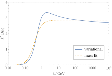
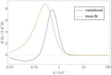
Figure 3: Left: The transversal gluon form factor $k^{2}/\omega(k)$ of our variational solution, compared to the best fit to the form factor of a massive propagator. Right: The integrand $[\phi^{\prime}(k)+k\phi^{\prime\prime}(k)]$ of the Hankel transform eq. (29) without the oscillating Bessel functions, again compared to the best massive fit to the form factor.

V Results

V.1 Free action

Let us first discuss the calculation of the free energy density as a function of the Polyakov loop background field in our variational model. We take the Poisson resummed formula eq. (27) and compute the Hankel transform $h(\lambda)$ from eq. (29), which is also the numerically challenging part as the integrand in its definition is strongly oscillating.

Let us first check whether we can replace the transversal gluon propagator $\omega(k)^{-1}$ by a massive propagator, since the Hankel transform for the latter can be done analytically. In the left panel of Fig. 3, we compare the form factor of the transversal propagator, $k^{2}/\omega(k)$, for our actual numerical solution of the variational problem with the best massive propagator fit. Clearly, the massive fit underestimates the propagator strength in the mid-momentum region, and it also misses the logarithmic decay of the propagator at large momenta. In the right panel of figure 3, we plot the integrand $[\phi^{\prime}(k)+k\phi^{\prime\prime}(k)]$ of the Hankel transform eq. (29) without the oscillating Bessel functions factor. For small momenta, the variational result becomes negative, a fact that will turn out to be important for the discussion of the pressure in the confined phase of our approach. By contrast, the integrand remains positive if we replace the propagator by the best fit to a free massive particle. .

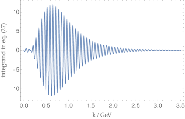
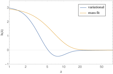
Figure 4: Left: The full integrand for the Hankel transform in eq. (29) for $\lambda=100$. Right: The Hankel transform $h(\lambda)$ from eq. (29) for the transversal modes in our variational solution, compared to the best massive fit, for which $h(\lambda)$ can be calculated analytically.

The full integrand in eq. (29) including the Bessel functions can be wildly oscillating, cf. Fig. 4, but the corresponding integral is still convergent and numerically treatable by standard techniques. The resulting function $h(\lambda)$ is plotted in the right panel of Fig. 4 for the non-perturbative transversal gluon degrees of freedom. (The perturbative ghosts and the longitudinal gluon can be treated analytically and merely add constants $\pm 1$ for each mode.) Clearly, $h(\lambda)$ is bounded, so that the series in eq. (27) is majorized by $\sum_{\nu}\nu^{-4}$ and hence converging very quickly; in practice, we rarely need to sum more than $10$ terms to compute $u(x,\beta)$ reliably.

Figure 5 shows the free energy $u(x,\beta)$ from eq. (27) as a function of the Polyakov loop background (21) for various temperatures. Although the analytical expression eq. (33) is clearly the correct high temperature limit, the approach to this limit is rather slow and still not fully reached for temperatures $T\approx 3T^{\ast}$. As we lower the temperature from the $T\to\infty$ limit, the potential $u(x,\beta)$ quickly moves downwards and essentially vanishes at criticality $T=T^{\ast}$. For even lower temperatures (i.e. within the confined phase), $u(x,\beta)$ first reaches the analytical limit (32) at around $T=0.7\,T^{\ast}$, before it overshoots the limit and reaches values well below eq. (32), before gradually moving up again and eventually settling on the limit eq. (32) from below.

The change of shape in $u(x,\beta)$ at $T<T^{\ast}$ is indispensable to enforce $x=1/2$ and hence confinement; it is due to the dominating ghost contribution at small temperatures. Since $u(x,\beta)$ essentially vanishes at criticality, the ghost dominance also implies that the free energy must become negative in the confinement region, which means that there is a positive pressure below $T^{\ast}$, in contrast to lattice calculation and physical expectations. In addition, the overshooting of the zero temeprature limit $u_{\infty}(x)$ even induces a shallow maximum of the pressure deep within the confining region. This can be traced back to the negative section of the Hankel transform $h(\lambda)$ in eq. (4), which in turn is related to the negative integrand in Fig. 3, and hence to the mid- and low-momentum behaviour of the gluon propagator. A free massive particle, by contrast, would start from the same high-temperature limit $u_{0}(x)$ for the free energy in Fig. 5 and also gradually move downwards, but eventually will settle on a flat profile from above, without ever turning negative or changing shape; in particular, it will have the minimum of the free energy at $x=0$ at all temperatures and thus show no confinement.

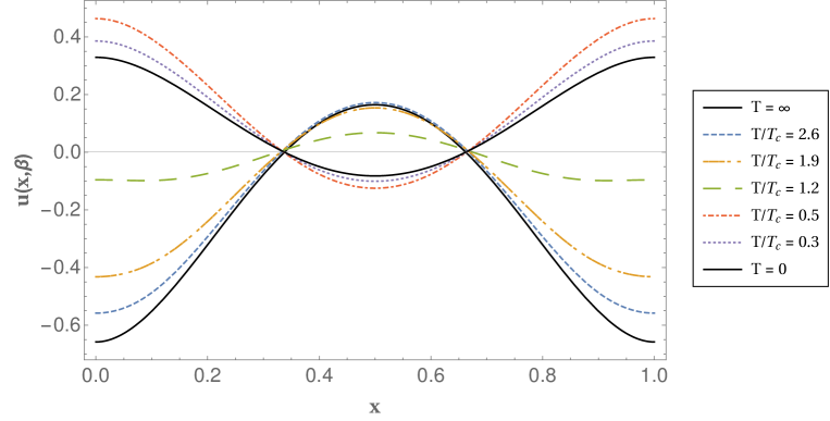
Figure 5: Left: The free energy $u(x,\beta)=\beta^{4}\,f_{\beta}(x)$ from eq. (27) as a function of the Polyakov loop background for various temperatures. The asymptotic limites at $T\to 0$ and $T\to\infty$ are taken from eqs. (32) and (33), respectively.

V.2 Pressure and thermodynamics

Figure 6 shows the pressure for our variational solution, as computed from the negative minimum of the free action density with respect to the Polyakov loop background $x$. In the left panel, we compare our solution with the SU(2) lattice data from Ref. Engels et al. (1989). We first observe that the Stefan-Boltzmann limit at large temperatures is correctly reproduced, as we have seen analytically above. The agreement with the SU(2) lattice data from Ref. Engels et al. (1989) is also fairly good over the entire deconfinement region $T>T^{\ast}$. At criticality $T=T^{\ast}$, the pressure vanishes which is caused by a compensation between the transversal gluons and the enhanced ghost degrees of freedom. As can be seen in the right panel of Fig. 6, a model of free massive bosons only would show the correct Stefan-Boltzmann and zero-temperature limit, but lacks any sign of a phase transition.

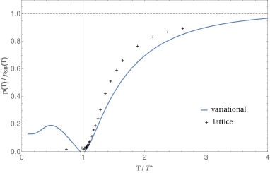
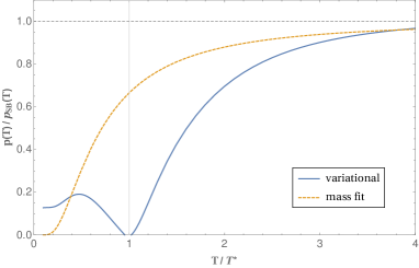
Figure 6: Left: The dimensionless pressure $p(T)/T^{4}$ of the variational solution, normalized to the Stefan-Boltzmann limit. In the left panel, our solution is compared to $SU(2)$ lattice data from Ref. Engels et al. (1989), while the right panel compares with a model of free massive bosons.

The situation is more complicated in the confinement region $T<T^{\ast}$: Here, the lattice only exhibits the true color-neutral excitations in the confined phase, which are glue-balls in the pure Yang-Mills theory, or baryons and mesons in full QCD. All these excitations have masses much larger than $T^{\ast}$, so that the free energy (and hence the pressure) as well as the energy density become exponentially suppressed in the entire confined region $T<T^{\ast}$. The lattice data in Fig. 6 confirms this expectation, although the data in the confined phase is very scarce. By contrast, the pressure in our variational solution increases again below $T^{\ast}$, to reach a small maximum around $T\approx 0.7\,T^{\ast}$, before decaying eventually towards the limit

$$\lim_{T\to 0}\frac{p(T)}{p_{\rm SB}(T)}=\frac{1}{8}\neq 0\,.$$ (36)

also seen e.g. in Ref. Reinosa et al. (2015).

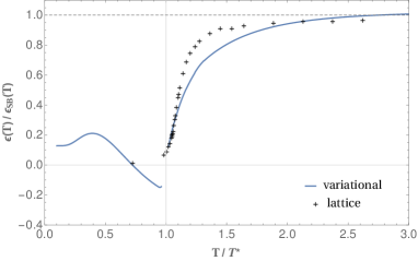
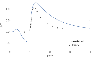
Figure 7: The energy density $\epsilon(T)/T^{4}$ (left) and the interaction strength (right) of our variational approach, compared to $SU(2)$ lattice data from Ref. Engels et al. (1989).

The behaviour in the confinement region is problematic since it leads e.g. to negative values of the energy density just below $T^{\ast}$, and moreover to a jump in the energy density not expected for a second order phase transition. Similar artifacts can be seen in the confined phase of practically all continuum formulations working directly with gluon fields, though approaches with a massive behaviour of the transversal gluon do not exhibit the small maximum of the pressure around $T\approx 0.7\,T^{\ast}$ seen in our calculation. In general, the numerical magnitude of the structure in the confined region (also quantified by the intercept eq. ()36) is rather small in our case compared to other continuum approaches Canfora et al. (2015); Kondo (2015), while our findings do resemble the results of massive loop calculations Reinosa et al. (2015).

In our approach, we can trace the unusual progression of the pressure in the confined region to the following two issues:

1. The region with a negative value for the Hankel transform (cf. Fig. 3) leads to an excessive minimum (overshooting) of the free energy around $T\approx 0.7\,T^{\ast}$ and hence to the small (unphysical) maximum of the pressure around that temperature.

2. The non-vanishing value eq. (36) at zero temperature must be due to the presence of massless modes, since only these modes can contribute to the ratio eq. (36) at $T\to 0$. No such massless excitations are, however, present in the full theory, and on the lattice, below $T^{\ast}$.

The first issue is, in fact, related to the maximum in the transversal gluon form factor at intermediate momenta. This is most easily demonstrated by replacing the form factor with a massive fit, as indicated in Fig. 3. The Hankel transform in Fig. 3 then remains positive. If we also keep the longitudinal and ghost degrees of freedom as well as the curvature (via the gap equation), the resulting pressure has a phase transition due to ghost dominance, but lacks any maximum in the confined region (see Fig. 8). On the lattice, the maximum in the gluon form factor is also seen, but it has no effect on the pressure for $T<T^{\ast}$ which is thoroughly suppressed by the large mass of all physical excitations. To turn this argument around, we can say that the presence of massless modes in the confined region makes the thermodynamics of our approach more sensitive to details of the gluon propagator at intermediate energies than it should.

V.3 Discussion

As mentioned above, the artifacts and partially unphysical features in the confined region are predominantly related to the presence of massless modes in our approach, even within the confined region. This is, to some extent, unavoidable in a continuum calculation, since e.g. the longitudinal gluon will always remain massless and will be present at all temperatures. In the exact theory, this gauge mode will receive no mass or other radiative corrections beyond one loop, but it will still be eliminated from the spectrum through cancellation by ghosts via BRST symmetry. This scenario cannot be fully accommodated in our approach. We have discussed the lack of BRST symmetry through the Gaussian ansatz (not the variation principle itself), and possible remedies or improvements in our previous work Refs. Quandt et al. (2014); Quandt and Reinhardt (2015, 2016). Obviously, the Gaussian ansatz is not able to model the real physical degrees of freedom (massive glue-balls) in the confined phase. In particular, the ghost dominance which is the mechanism for confinement preferred by the variational principle, automatically leads to the presence of massless coloured degrees of freedom at low temperatures, which in turn induce a non-vanishing pressure in the confined phase. A full BRST invariant treatment would presumably display a very different confinement mechanism based on colourless, massive excitations and BRST invariant states. It is clear that our Gaussian ansatz cannot accommodate this scenario and the effect of spurious massless gauge modes cannot be fully avoided. These undesirable consequences of BRST breaking may be less prominent in other observables, but the thermodynamics is very sensitive to it, as it predominantly counts massless degrees of freedom at very small temperatures.

Several remedies for this situation come to mind. The massless modes dominantly affect the Hankel transform limit $h_{\infty}\equiv\lim\limits_{\lambda\to\infty}h(\lambda)$, which should vanish in the full theory. Since the limit is non-uniform, any (infinitesimally small) mass $\mu$ for the longitudinal and ghost modes would enforce the correct limit $P(T)/T^{4}\to 0$ at $T\to 0$. However, this would only affect the temperature region $T<\mu$ and will not solve the issue in the entire confined region. What would be required is a rather large mass $\mu\gg T^{\ast}$ that only exists in the confined region. The variational solution does not seem to favour this scenario (and it is forbidden for the longitudinal gluon anyway).

A second method would be to declare the massless modes as unphysical and stipulate that their contribution to $h_{\infty}$ should be removed. This can easily be implemented by subtracting $h(\lambda)\to h(\lambda)-h_{\infty}$, which automatically yields $h(\infty)=0$ and the correct limit at very small temperatures. However, this removal is only warranted if the massless modes have been identified spurious over the entire temperature range, which is not the case in the deconfined region. While the removal of the zero modes gives a very good description of the lattice data up to temperatures of about $2T^{\ast}$ (see Fig. 8), it will eventually overshoot the Stefan-Boltzmann limit at $T\to\infty$ because some of the massless modes in the deconfined region are eliminated as well. Clearly, some way of restricting the removal to the confined region would be necessary, and we see currently no way of implementing this consistently in the variational ansatz.

Thirdly, we could generally improve on the violation of BRST symmetry by extending the variational measure beyond the Gaussian ansatz through either gluon interaction with non-trivial vertices or even explicit glue ball degrees of freedom. The latter could be implemented through additional dialton fields e.g. along the lines of Ref. Sasaki and Redlich (2012). Non-Gaussian measures, on the other hand, would allow to dress the vertices in agreement with Slavnov-Taylor identities, but it could also accommodate gluon bound states through non-linear field equations. The techniques for dealing with non-Gaussian measures have already been explored in Refs. Campagnari and Reinhardt (2015, 2010) for the case of the Hamiltonian approach. It can straightforwardly adapted to the present case, where the gap equations for the vertices provided additional optimizations. This third approach is clearly the most physical and its implementation will be discussed elsewhere.

In the deconfined region $T\geq T^{\ast}$, our ansatz displays the right degrees of freedom and our variational solution describes the physics of the gluon plasma quite accurately. In particular, it exhibits a pressure that drops to zero at or near the critical temperature $T^{\ast}$, and an energy density which approaches its Stefan-Boltzmann limit much faster than the pressure (compare Fig. 6 and Fig. 7). In addition, it also shows a clear maximum of the interaction strength just above the critical temperature at around $T\approx 1.25\,T^{\ast}$, which is only slightly larger than the lattice findings of $T=1.2\,T^{\ast}$. Both the approach towards the Stefan-Boltzmann limit, and the fast decay of the interaction strength at higher temperatures are somewhat underestimated in our variational solution, but the overall agreement with the lattice is still fairly good, given the simplicity of our method.

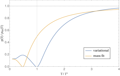
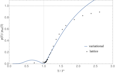
Figure 8: Left: The dimensionless pressure $p(T)/T^{4}$ normalized to the Stefan-Boltzmann limit, compared to a model in which the transversal gluon form factor has been replaced by a mass fit, but longitudinal gluons, ghosts and curvature are fully retained. Right: The pressure $P(T)/T^{4}$ with removal of (spurios) massless modes, compared to lattice data Engels et al. (1989).

VI Conclusions

In this paper, we have investigated the thermodynamics of $SU(2)$ Yang-Mills theory in the covariant variational approach. With the properly subtracted free energy, we find a pressure for the gluon plasma which yields good agreement with the lattice data over the entire deconfinement region, including the correct Stefan-Boltzmann limit at $T\to\infty$. There is a clear phase transition at which the pressure drops to zero, and the interaction strength shows a pronounced maximum just above $T^{\ast}$, as is also expected from the lattice. In the confined region, the mechanism of ghost dominance and spurious massless modes due to the lack of full BRST symmetry make their appearance and the pressure is not fully suppressed. Instead, it even shows a shallow maximum around $0.7\,T^{\ast}$ before settling to a non-vanishing value for $p(T)/T^{4}$ at $T\to 0$, also in contrast to lattice findings (but in agreement with most continuum methods). Such effects are unphysical and lead to jumps in the energy density and interaction strength, and even a small temperature range of negative energy density. We have attempted to identify the reason for these problems and discussed possible remedies. To overcome these issues, our variational ansatz must be enlarged to include either higher vertices and non-linear gluon interactions, or glue-ball degrees of freedom directly.

A similar extension of the Gaussian ansatz also becomes necessary when quark degrees of freedom are introduced and eventually coupled to a chemical potential, as the corresponding vertices will be heavily dressed. The development of Dyson-Schwinger techniques for this formulation in analogy to the variational Hamiltonian approach Campagnari and Reinhardt (2015, 2010) are currently under investigation.

Appendix A Poisson resummation

In this appendix, we derive eq. (27). We start from expression (22) for the free action density, which we write

$$\beta^{4}f_{\beta}(x)=4\pi\int_{0}^{\infty}dq\,q^{2}\sum_{n\in\mathbb{Z}}\Bigg{[}\phi\Big{(}\frac{2\pi}{\beta}\sqrt{(n+x)^{2}+q^{2}}\Big{)}+\frac{1}{2}\,\phi\Big{(}\frac{2\pi}{\beta}\sqrt{n^{2}+q^{2}}\Big{)}\Bigg{]}\,,$$ (37)

with the function $\phi(k)$ defined in eq. (27). After Poisson resummation, we obtain

$$\beta^{4}f_{\beta}(x)=4\pi\int_{0}^{\infty}dq\,q^{2}\int_{-\infty}^{\infty}dz\sum_{\nu\in\mathbb{Z}}e^{2\pi i\nu z}\,\Bigg{[}\phi\Big{(}\frac{2\pi}{\beta}\sqrt{(z+x)^{2}+q^{2}}\Big{)}+\frac{1}{2}\,\phi\Big{(}\frac{2\pi}{\beta}\sqrt{z^{2}+q^{2}}\Big{)}\Bigg{]}\,.$$ (38)

As explained in the main text, the $\nu=0$ term describes a space-time constant, temperature and background field independent contribution $\delta f$, which is part of the free energy density at any temperature. It can readily be identified as the divergent vacuum action density which is to be expected on general grounds and should be removed by a cosmological constant type of counter term. After omitting this term, we can change variables $s=z+x$ and combine terms with $\pm\nu$ to find

$$\beta^{4}f_{\beta}(x)=4\pi\sum_{\nu=1}^{\infty} \Bigg{[}e^{-2\pi i\nu x}\int_{0}^{\infty}dq\,q^{2}\int_{-\infty}^{\infty}ds\,\phi\Big{(}\frac{2\pi}{\beta}\sqrt{s^{2}+q^{2}}\Big{)}\,e^{2\pi i\nu s}$$

$$+e^{2\pi i\nu x}\int_{0}^{\infty}dq\,q^{2}\int_{-\infty}^{\infty}ds\,\phi\Big{(}\frac{2\pi}{\beta}\sqrt{s^{2}+q^{2}}\Big{)}\,e^{-2\pi i\nu s}$$

$$+\big{(}e^{2\pi i\nu s}+e^{-2\pi i\nu s}\big{)}\,\frac{1}{2}\,\int_{0}^{\infty}dq\,q^{2}\int_{-\infty}^{\infty}ds\,\phi\Big{(}\frac{2\pi}{\beta}\sqrt{s^{2}+q^{2}}\Big{)}\Bigg{]}\,.$$ (39)

Changing variables $s\to(-s)$ in the second and third term gives

$$\beta^{4}f_{\beta}(x)=8\pi\sum_{\nu=1}^{\infty}\Big{[}\cos(2\pi\nu x)+\frac{1}{2}\Big{]}\int_{0}^{\infty}dqq^{2}\int_{-\infty}^{\infty}ds\,\phi\Big{(}\frac{2\pi}{\beta}\sqrt{s^{2}+q^{2}}\Big{)}\,e^{2\pi i\nu s}\,.$$ (40)

The integrand is even in $q$ and we can extend the $q$-integral to all of $\mathbb{R}$. Next we introduce polar coordinates $(r,\varphi)$ in the $(q,s)$-plane and find

$$\beta^{4}f_{\beta}(x) =4\pi\sum_{\nu=1}^{\infty}\Big{[}\cos(2\pi\nu x)+\frac{1}{2}\Big{]}\int_{0}^{\infty}dr\,r\int_{0}^{2\pi}d\varphi\,r^{2}\sin^{2}\varphi\cdot\phi\big{(}2\pi r/\beta\big{)}\,e^{2\pi ir\nu\cos\varphi}$$

$$=4\pi\sum_{\nu=1}^{\infty}\Big{[}\cos(2\pi\nu x)+\frac{1}{2}\Big{]}\int_{0}^{\infty}dr\,r^{3}\,\phi\big{(}2\pi r/\beta\big{)}\,\int_{0}^{2\pi}d\varphi\,\sin^{2}\varphi\cdot e^{2\pi ir\nu\cos\varphi}$$

$$=4\pi\sum_{\nu=1}^{\infty}\Big{[}\cos(2\pi\nu x)+\frac{1}{2}\Big{]}\int_{0}^{\infty}dr\,r^{2}\,\phi\big{(}2\pi r/\beta\big{)}\,\frac{J_{1}(2\pi\nu r)}{\nu}\,.$$ (41)

A final change of variables $\tau\equiv 2\pi\nu r$ yields

$$\beta^{4}f_{\beta}(x) =\frac{1}{2\pi^{2}}\sum_{\nu=1}^{\infty}\frac{\cos(2\pi\nu x)+\frac{1}{2}}{\nu^{4}}\int_{0}^{\infty}d\tau\,\tau^{2}\,J_{1}(\tau)\,\phi(\tau/(\nu\,\beta))\,.$$ (42)

If we abbreviate the Hankel transform by

$$h(\lambda)=-\frac{1}{4}\,\int_{0}^{\infty}d\tau\,\tau^{2}\,J_{1}(\tau)\,\phi(\tau/\lambda)$$ (43)

we arrive eventually at eq. (27) from the main text.

Appendix B Hankel transformation

We want to compute the Hankel transformation eq. (28) in the main text,

$$h(\lambda)=-\frac{\lambda^{3}}{4}\int_{0}^{\infty}dk\,k^{2}\,J_{1}(\lambda k)\,\phi(k)\,,$$ (44)

where we first assume that the integrand $\phi(k)$ is regular at the origin and vanishes fast enough at large $k$ so that the integral converges. In this case, we can integrate by parts twice to obtain

$$h(\lambda)=\frac{1}{4}\,\int_{0}^{\infty}dk\,\left(2J_{0}(\lambda k)+\lambda k\,J_{1}(\lambda k)\right)\cdot\left(k\phi^{\prime\prime}(k)+\phi^{\prime}(k)\right)\,,$$ (45)

which is eq. (29) from the main text. This formula has the advantage, that it converges for functions $\phi(k)$ which have a much weaker decay at large $k$, or even a mild (logarithmic) increase at $k\to\infty$.

We can view eq. (45) as an analytical continuation of the initial formula (44) which can be justified by density arguments in many cases. More explicitly, we can regularize the original integral (44) in a distributional sense by replacing $\phi(k)\to\phi(k)\cdot e^{-\mu k}$ with $\mu>0$, and consider

$$h(\lambda)=\lim_{\mu\to+0}\frac{\lambda^{3}}{4}\int_{0}^{\infty}dk\,k^{2}\,J_{1}(\lambda k)\,\phi(k)\cdot e^{-\mu k}\,.$$ (46)

Integrating by parts twice yields for the integral without the limit

$$- \Big{[}\frac{(\lambda k)^{2}}{4}\,J_{2}(\lambda k)\,\phi(k)+\frac{k}{4}\,[\phi^{\prime}(k)-\mu\phi(k)]\cdot[2J_{0}(\lambda k)+\lambda k\,J_{1}(\lambda k)]\Big{]}\cdot e^{-\mu k}\Bigg{|}_{0}^{\infty}$$

$$+ \frac{1}{4}\int_{0}^{\infty}dk\,[2J_{0}(\lambda k)+\lambda k\,J_{1}(\lambda k)]\cdot[k\phi^{\prime\prime}(k)+(1-2\mu k)\phi^{\prime}(k)+\mu(\mu k-1)\,\phi(k)]\cdot e^{-\mu k}\,.$$ (47)

If $\phi(k)$ is regular at the origin, the boundary contribution from $k=0$ vanishes; likewise, the boundary contribution from $k=\infty$ vanishes due to the common factor $e^{-\mu k}$, provided that $\phi(k)$ only has a mild divergence at $k\to\infty$. In this case,

$$(\ref{hankelreg})=\lim_{\mu\to+0}\frac{1}{4}\int_{0}^{\infty}dk\,[2J_{0}(\lambda k)+\lambda k\,J_{1}(\lambda k)]\cdot[k\phi^{\prime\prime}(k)+(1-2\mu k)\phi^{\prime}(k)+\mu(\mu k-1)\,\phi(k)]\cdot e^{-\mu k}$$

and the limit can be done under the integral, which leads to eq. (45).

We note in passing that the distributional limit is important: if we put $\mu=0$ in eq. (46) and instead regularize the integral by a cutoff $\Lambda$, then the boundary term in eq. (47) will not vanish unless the the cutoff is taken to infinity as the special sequence $\Lambda_{n}=u_{n}/\lambda$, where $u_{n}\approx\pi(\frac{5}{4}+n)$ is the nth zero of the Bessel function $J_{2}(x)$. For this sequence of cutoffs $\Lambda_{n}\to\infty$, the first boundary term in eq. (47) vanishes, while the second one becomes independent of $\lambda$. The result would then again be eq. (45), however with an additional constant $h_{0}$ on the rhs, which only vanishes if $\phi^{\prime}(k)\sim k^{-(1+\epsilon)}$ at large $k$. The distributional argument has the merit of extending eq. (45) to a wider class of functions with stronger divergence at $k\to\infty$.

Appendix C Massive free bosons

To check the results from appendix B, let us study a single scalar boson of mass $m$ with dispersion relation $\omega(k)=k^{2}+m^{2}$, i.e. we consider

$$\phi(k)=\ln\frac{\omega(k)}{\mu^{2}}=\ln\frac{k^{2}+m^{2}}{\mu^{2}}\,,$$

where the scale $\mu$ is arbitrary and not to be confused with the regulator in appendix B. The model function $\phi(k)$ has only a mild (logarithmic) divergence at $k\to\infty$ and eq. (45) leads to a Hankel-Nicholson type of integral,

$$h(\lambda) =\frac{1}{4}\,\int_{0}^{\infty}dk\,\Big{[}2J_{0}(\lambda k)+\lambda k\,J_{1}(\lambda k)\Big{]}\cdot\frac{4km^{2}}{(k^{2}+m^{2})^{2}}$$

$$=(\lambda m)^{2}\,\int_{0}^{\infty}dq\,\big{(}2J_{0}(q)+qJ_{1}(q))\,\frac{q}{(q^{2}+(\lambda m)^{2})^{2}}$$

$$=\frac{1}{2}\,(\lambda m)^{2}\,K_{2}(\lambda m)\,.$$ (48)

Here, $K_{2}$ is a modified Bessel function and the result is indeed independent of the scale $\mu$. In the massless limit $m\to 0$, we recover the simple result $h(\lambda)=1$.

References

- Fischer (2006) C. S. Fischer, J.Phys. G32, R253 (2006), arXiv:hep-ph/0605173 [hep-ph] .
- Alkofer and von Smekal (2001) R. Alkofer and L. von Smekal, Phys.Rept. 353, 281 (2001), arXiv:hep-ph/0007355 [hep-ph] .
- Binosi and Papavassiliou (2009) D. Binosi and J. Papavassiliou, Phys.Rept. 479, 1 (2009), arXiv:0909.2536 [hep-ph] .
- Tissier and Wschebor (2010) M. Tissier and N. Wschebor, Phys. Rev. D82, 101701 (2010), arXiv:1004.1607 [hep-ph] .
- Tissier and Wschebor (2011) M. Tissier and N. Wschebor, Phys. Rev. D84, 045018 (2011), arXiv:1105.2475 [hep-th] .
- Zwanziger (1989) D. Zwanziger, Nucl. Phys. B323, 513 (1989).
- Zwanziger (1993) D. Zwanziger, Nucl. Phys. B399, 477 (1993).
- Canfora et al. (2015) F. E. Canfora, D. Dudal, I. F. Justo, P. Pais, L. Rosa, and D. Vercauteren, Eur. Phys. J. C75, 326 (2015), arXiv:1505.02287 [hep-th] .
- Pawlowski (2007) J. M. Pawlowski, Annals Phys. 322, 2831 (2007), arXiv:hep-th/0512261 [hep-th] .
- Gies (2012) H. Gies, Lect.Notes Phys. 852, 287 (2012), arXiv:hep-ph/0611146 [hep-ph] .
- Feuchter and Reinhardt (2004) C. Feuchter and H. Reinhardt, (2004), arXiv:hep-th/0402106 [hep-th] .
- Reinhardt and Feuchter (2005) H. Reinhardt and C. Feuchter, Phys.Rev. D71, 105002 (2005), arXiv:hep-th/0408237 [hep-th] .
- Epple et al. (2007) D. Epple, H. Reinhardt, and W. Schleifenbaum, Phys.Rev. D75, 045011 (2007), arXiv:hep-th/0612241 [hep-th] .
- Quandt et al. (2014) M. Quandt, H. Reinhardt, and J. Heffner, Phys.Rev. D89, 065037 (2014), arXiv:1310.5950 [hep-th] .
- Quandt and Reinhardt (2015) M. Quandt and H. Reinhardt, Phys. Rev. D92, 025051 (2015), arXiv:1503.06993 [hep-th] .
- Quandt and Reinhardt (2016) M. Quandt and H. Reinhardt, Phys. Rev. D94, 065015 (2016), arXiv:1603.08058 [hep-th] .
- Fischer et al. (2011) C. S. Fischer, J. Luecker, and J. A. Mueller, Phys. Lett. B702, 438 (2011), arXiv:1104.1564 [hep-ph] .
- Fischer and Luecker (2013) C. S. Fischer and J. Luecker, Phys. Lett. B718, 1036 (2013), arXiv:1206.5191 [hep-ph] .
- Reinosa et al. (2015) U. Reinosa, J. Serreau, M. Tissier, and N. Wschebor, Phys.Rev. D91, 045035 (2015), arXiv:1412.5672 [hep-th] .
- Reinosa et al. (2016) U. Reinosa, J. Serreau, M. Tissier, and N. Wschebor, Phys. Rev. D93, 105002 (2016), arXiv:1511.07690 [hep-th] .
- Fukushima and Su (2013) K. Fukushima and N. Su, Phys. Rev. D88, 076008 (2013), arXiv:1304.8004 [hep-ph] .
- Zwanziger (2005) D. Zwanziger, Phys. Rev. Lett. 94, 182301 (2005), arXiv:hep-ph/0407103 [hep-ph] .
- Reinhardt and Heffner (2017a) H. Reinhardt and J. Heffner, (2017a), in preparation.
- Reinhardt (2016) H. Reinhardt, Phys. Rev. D94, 045016 (2016), arXiv:1604.06273 [hep-th] .
- Reinhardt and Heffner (2017b) H. Reinhardt and J. Heffner, (2017b), in preparation.
- Bernard (1974) C. W. Bernard, Phys.Rev. D9, 3312 (1974).
- Bogolubsky et al. (2009) I. Bogolubsky, E. Ilgenfritz, M. Muller-Preussker, and A. Sternbeck, Phys.Lett. B676, 69 (2009), arXiv:0901.0736 [hep-lat] .
- Braun et al. (2010) J. Braun, H. Gies, and J. M. Pawlowski, Phys. Lett. B684, 262 (2010), arXiv:0708.2413 [hep-th] .
- Taylor (1971) J. Taylor, Nucl.Phys. B33, 436 (1971).
- Ilgenfritz et al. (2007) E. M. Ilgenfritz, M. Muller-Preussker, A. Sternbeck, A. Schiller, and I. L. Bogolubsky, Braz. J. Phys. 37, 193 (2007), arXiv:hep-lat/0609043 [hep-lat] .
- Sternbeck (2006) A. Sternbeck, The Infrared behavior of lattice QCD Green’s functions, Ph.D. thesis, Humboldt U., Berlin (2006), arXiv:hep-lat/0609016 [hep-lat] .
- Lucini et al. (2004) B. Lucini, M. Teper, and U. Wenger, JHEP 01, 061 (2004), arXiv:hep-lat/0307017 [hep-lat] .
- Engels et al. (1989) J. Engels, J. Fingberg, K. Redlich, H. Satz, and M. Weber, Z. Phys. C42, 341 (1989).
- Karsch and Laermann (2003) F. Karsch and E. Laermann, (2003), arXiv:hep-lat/0305025 [hep-lat] .
- Kondo (2015) K.-I. Kondo, (2015), arXiv:1508.02656 [hep-th] .
- Sasaki and Redlich (2012) C. Sasaki and K. Redlich, Phys. Rev. D86, 014007 (2012), arXiv:1204.4330 [hep-ph] .
- Campagnari and Reinhardt (2015) D. R. Campagnari and H. Reinhardt, Phys. Rev. D92, 065021 (2015), arXiv:1507.01414 [hep-th] .
- Campagnari and Reinhardt (2010) D. R. Campagnari and H. Reinhardt, Phys.Rev. D82, 105021 (2010), arXiv:1009.4599 [hep-th] .