Relative periodic orbits form the backbone of turbulent pipe flow

Abstract

Chaotic dynamics of low-dimensional systems, such as Lorenz or Rössler flows, is guided by the infinity of periodic orbits embedded in their strange attractors. Whether this also be the case for the infinite-dimensional dynamics of Navier–Stokes equations has long been speculated, and is a topic of ongoing study. Periodic and relative periodic solutions have been shown to be involved in transitions to turbulence. Their relevance to turbulent dynamics—specifically, whether periodic orbits play the same role in high-dimensional nonlinear systems like the Navier–Stokes equations as they do in lower-dimensional systems—is the focus of the present investigation. We perform here a detailed study of pipe flow relative periodic orbits with energies and mean dissipations close to turbulent values. We outline several approaches to reduction of the translational symmetry of the system. We study pipe flow in a minimal computational cell at $Re=2500$, and report a library of invariant solutions found with the aid of the method of slices. Detailed study of the unstable manifolds of a sample of these solutions is consistent with the picture that relative periodic orbits are embedded in the chaotic saddle and that they guide the turbulent dynamics.

1 Introduction

Revealing the underlying mechanisms of fluid turbulence is a multidisciplinary endeavour that brings together pure and applied mathematics, high performance computation, and experimental physics. Over the past two decades, this effort has led to significant progress in our understanding of transitionally turbulent fluid flows in physically motivated geometries, such as a circular pipe. Today we have numerical evidence that the laminar state of the pipe flow (Hagen, 1839; Poiseuille, 1840) is linearly stable for all cases that can be observed in laboratory experiments, i.e., for Reynolds numbers up to $\textit{Re}=10^{7}$ (Meseguer & Trefethen, 2003). In addition, both numerical and laboratory experiments (Avila et al., 2010; Hof et al., 2006) indicate that turbulence of finite spatial extent, either in the form of a localised patch or turbulence or within a geometry of finite volume, has a finite lifetime at transitional Re values. (When the spatial expansion of turbulence in larger domains defeats relaminarisations, such that it persists indefinitely, the system becomes a strange attractor; Avila et al. (2011).) These observations suggest, from the dynamical systems point of view, that the study of a turbulent pipe flow is the study of a chaotic saddle, i.e., a strange repeller in the infinite-dimensional state space of the solutions to Navier–Stokes equations. For low-dimensional dynamics, it is known that strange sets are shaped by the ‘invariant solutions’ and their stable and unstable manifolds.

This intuition motivated several groups (Faisst & Eckhardt, 2003; Wedin & Kerswell, 2004; Pringle & Kerswell, 2007; Willis et al., 2013) to investigate invariant solutions of Navier–Stokes equations in a circular pipe; these studies, in turn, were followed by experimental observations (Hof et al., 2004; Dennis & Sogaro, 2014) of relatively close visits of the turbulent trajectories to some of the numerical travelling wave solutions. With a fast-growing catalogue of exact invariant solutions of the Navier–Stokes equations in hand, acquired by our group and others (Willis et al., 2016; Gibson, 2017), we are nearing the point where focus turns from finding invariant solutions to constructing their stable and unstable manifolds, the building blocks of a chaotic saddle.

Most of the early studies of invariant solutions in pipe flow had focused on structures that play role in transition to turbulence. Typically these solutions emerged in saddle-node bifurcations (or further bifurcations of such solutions) as lower/upper-branch pairs. Lower-branch solutions appeared to belong to state space regions that separated initial conditions into those that uneventfully relaminarize, and those that develop into turbulence. Moreover, these solutions are characterized by structures smoother than those observed in turbulence, hence their numerical study was relatively simple and required moderate numbers of computational degrees of freedom. Upper-branch solutions, on the other hand, undergo very complex sequences of bifurcations  (Mellibovsky & Eckhardt, 2012) upon increasing Re, giving rise to complicated dynamics with many of the resulting solutions distant from the turbulent regions. While these bifurcations are precursors of turbulence in pipe flow, a complete continuation from upper-branch solutions to turbulence is a very hard task: Many solutions undergo sequences of bifurcations in different regions of the state space, then sometimes merge through boundary crises that are hard to detect.

By contrast, the strategy of the present study is to extract invariant solutions from close recurrences of turbulent flow simulations (Auerbach et al., 1987), for a given Re and domain geometry, with the aim of identifying dynamically relevant structures, without any prior knowledge of the bifurcation sequences from which they might have originated.

Pipe flow is driven by a pressure gradient; hence, all of its finite-amplitude solutions drift downstream. The simplest invariant solutions in such translationally-invariant systems are travelling waves. Due to the azimuthal-rotation invariance of the pipe flow, in general one anticipates finding travelling waves that simultaneously drift downstream and rotate about the axis of the pipe (rotational waves). Since the motions of such solutions can be eliminated by a change to the co-moving frame, moving along the system’s symmetry directions, the physical observables associated with them, such as wall friction or dissipation, do not change in time. In other words, the dynamical information contained in these solutions is rather limited. The simplest time-dependent invariant solutions that capture dynamics in terms of time-dependent, but symmetry-invariant, observables are the relative periodic orbits, which are velocity field profiles that exactly recur at a streamwise (downstream) shifted location after a finite time. More generally, relative periodic orbits may have azimuthal rotations in addition to the streamwise drifts, however, such orbits are not contained in the symmetry-subspace we study here.

In this work, we present the 48 relative periodic orbits and $10$ travelling waves, adding $19$ new solutions to the $29$ solutions reported in Willis et al. (2016). Six of these new relative periodic orbits are computed by the method of multi-point shooting (for the first time in the pipe flow context) whereby the initial guesses for longer orbits are constructed from known shorter orbits that shadow them (see § A).

Next, we investigate the role the invariant solutions play in shaping the turbulent dynamics. To this end we carry out global and local state space visualizations, both in the symmetry-reduced state space, and in its Poincaré sections. For global visualizations, we take a data-driven approach and project relative periodic orbits and turbulent dynamics onto ‘principal components’ obtained from the symmetry-reduced turbulence data. We show that this approach has only limited descriptive power for explaining the organization of solutions in the state space. We then move onto examining the unstable manifold of our shortest relative periodic orbit and illustrate how it shapes the nearby solutions. This computation extends  Budanur & Hof (2017)’s method for studying the unstable manifolds of ‘edge state’ relative periodic orbits to the solutions that are embedded in turbulence, with unstable manifold dimensions greater than one. Finally, we demonstrate that when a turbulent trajectory visits the neighbourhood of this relative periodic orbit, it shadows it for a finite time interval.

Our results demonstrate the necessity of symmetry reduction for state space analysis. We reduce the continuous translational symmetry along the pipe by bringing all states to a symmetry-reduced state space (the slice), and contrast this with the ‘method of connections’. The remaining discrete azimuthal symmetry is reduced by defining a fundamental domain within the slice, where each state has a unique representation. We demonstrate, on concrete examples, that this symmetry reduction makes possible a dynamical analysis of the pipe flow’s state space.

The paper is organized as follows. In § 2 we describe the pipe flow and its symmetries. In § 3 we discuss the method of slices used to reduce the continuous symmetry. The computed invariant solutions are listed and discussed in § 4. In § 5 we investigate the dynamical role of the invariant solutions using global and local state space visualizations. Section § 6 contains our concluding remarks.

2 Pipe flow

The flow of an incompressible viscous fluid through a pipe of circular cross-section is considered. Fluid in a long pipe carries large momentum, which in turn smooths out fluctuations in the mass flux on short time-scales. We therefore consider flow with constant mass flux whose governing equations read

$$\frac{\partial\mbox{\boldmath$u$}}{\partial t}+\mbox{\boldmath$U$}\cdot\mbox{\boldmath$\nabla$}\mbox{\boldmath$u$}+\mbox{\boldmath$u$}\cdot\mbox{\boldmath$\nabla$}\mbox{\boldmath$U$}+\mbox{\boldmath$u$}\cdot\mbox{\boldmath$\nabla$}\mbox{\boldmath$u$}=-{\mbox{\boldmath$\nabla$}}p+32\frac{\beta}{\textit{Re}}\hat{{\bf z}}+\frac{1}{\textit{Re}}{\mbox{\boldmath$\nabla$}}^{2}\mbox{\boldmath$u$}\,,\qquad\mbox{\boldmath$\nabla$}\cdot\mbox{\boldmath$u$}=0\,.$$ (1)

The equations are formulated in cylindrical-polar coordinates $(r,\theta,z)$ denoting the radial coordinate $r$, the azimuthal angle $\theta$ and the stream-wise (or axial) coordinate $z$ along the pipe. The Reynolds number is defined as $\textit{Re}=UD/\nu$, where $U$ is the mean velocity of the flow, $D$ is the pipe diameter, and $\nu$ is the kinematic viscosity. The governing equation (1) is non-dimensionalized by scaling the lengths by $D$, the velocities by $U$, and time by $D/U$. The velocity $\mbox{\boldmath$u$}=(u,v,w)$ denotes the deviation from the dimensionless laminar Hagen–Poiseuille flow equilibrium $\mbox{\boldmath$U$}(r)=2\,(1-(2r)^{2})\,\hat{\mbox{\boldmath$z$}}$. In addition to the pressure gradient required to maintain laminar flow, the excess pressure required to maintain constant mass flux is measured by the feedback variable $\beta=\beta(\mbox{\boldmath$u$})$ — the total dimensionless pressure gradient is $(1+\beta)(32/Re)$ and $\beta=0$ for laminar flow. The Reynolds number used throughout this work is $Re=2500$.

Our computational cell is in the $m_{0}=4$ rotational subspace, $\Omega:(r,\theta,z)\in[0,\frac{1}{2}]\times[0,\frac{\pi}{2}]\times[0,\frac{\pi}{\alpha}]$ with $\alpha=1.7$, or in wall units for the wall-normal, spanwise and streamwise dimensions respectively, $\Omega^{+}\approx[100,160,370]$. The variables in (1) are discritised on $N$ non-uniformly spaced points in radius, with higher resolution near the wall, and with Fourier modes with index $|m|<M$ and $|k|<K$ in $\theta$ and $z$ respectively. Our resolution is $(N,M,K)=(64,12,18)$, so that following the $\frac{3}{2}$-rule, variables are evaluated on $64\times 36\times 54$ grid points, $(\Delta\theta\,D/2)^{+}\approx 5$ and $\Delta z^{+}\approx 7$. Whilst this domain is small, it is sufficiently large to reproduce the wall friction observed for the infinite domain to within 10%, and already sufficiently large to exhibit a complex array of periodic orbits (see Willis et al. (2016) for details.)

2.1 Symmetries of the pipe flow

Here we briefly review the symmetries of the problem, and then focus on the properties of the shift-and-reflect flow-invariant subspace, to which we restrict the study that we present in this article. For a detailed discussion of flow-invariant subspaces of the pipe flow see, for example, the Appendix of Willis et al. (2013). It will be seen presently that the shift-and-reflect symmetry leads to two dynamically equivalent regions of state space, later observed in simulations.

In pipe flow the cylindrical wall restricts the rotation symmetry to rotation about the $z$-axis, and translations along it. Let $g({\phi},\ell)$ be the shift operator such that $g({\phi},0)$ denotes an azimuthal rotation by ${\phi}$ about the pipe axis, and $g(0,\ell)$ denotes the stream-wise translation by $\ell$; let $\sigma$ denote reflection about the $\theta=0$ azimuthal angle:

$$g({\phi},\ell)\,[u,v,w,p](r,\theta,z) = [u,v,w,p](r,\theta-{\phi},z-\ell)$$

$$\sigma\,[u,v,w,p](r,\theta,z)\;\; = [u,-v,w,p](r,-\theta,z)\,.$$ (2)

The symmetry group of stream-wise periodic pipe flow is $\textrm{SO}(2)_{z}\times\textrm{O}(2)_{\theta}$; in this paper we restrict our investigations to dynamics restricted to the ‘shift-and-reflect’ symmetry subspace

$$S=\{e,\sigma g_{z}\}\,,$$ (3)

where $g_{z}$ denotes a streamwise shift by $L/2$, i.e., flow fields (2) that satisfy

$$[u,v,w,p](r,\theta,z)=[u,-v,w,p](r,-\theta,z-L/2)\,.$$ (4)

This requirement couples the stream-wise translations with the azimuthal reflection. It is worth emphasising that by imposing the symmetry $S$, continuous rotations in $\theta$ are prohibited. Hence we consider only the simplest example of a continuous group for the stream-wise translations, i.e. the one-parameter rotation group $\textrm{SO}(2)_{z}$, omitting the subscript $z$ whenever that leads to no confusion. In the azimuthal direction only a discrete rotation by half the spanwise periodicity is allowed, i.e. by $\pi/m_{0}$. We illustrate this property in figure 1.

Figure 1: (a) Sketch of a shift-and-reflect symmetric state in the doubly-periodic domain $(\theta,z)\in[-\math@atom{\pi}{\mathchoice{\hbox{$\displaystyle\pi$}}{\hbox{$\textstyle\pi$}}{\hbox{$\scriptstyle\pi$}}{\hbox{$\scriptscriptstyle\pi$}}}/m_{0},\math@atom{\pi}{\mathchoice{\hbox{$\displaystyle\pi$}}{\hbox{$\textstyle\pi$}}{\hbox{$\scriptstyle\pi$}}{\hbox{$\scriptscriptstyle\pi$}}}/m_{0}]\times[0,L]$ (same after shift by $L/2$ in $z$ followed by reflection across the dotted line $\theta=0$). (b) In general, if the state in (a) is rotated by an angle $\phi$, then the shift-and-reflect symmetry is broken. (c) However, the state in (a) rotated by the half-shift $\phi=\math@atom{\pi}{\mathchoice{\hbox{$\displaystyle\pi$}}{\hbox{$\textstyle\pi$}}{\hbox{$\scriptstyle\pi$}}{\hbox{$\scriptscriptstyle\pi$}}}/m_{0}$ remains in the shift-and-reflect subspace.

Thus, the symmetry group $G$ of the pipe flow in the shift-and-reflect subspace is

$$G=\{g_{\theta},\,g_{z}(l)\}\,,$$ (5)

where $g_{\theta}$ denotes the discrete azimuthal shift by $\pi/m_{0}$ and $g_{z}(l)=g(0,l)$.

Solutions that can be mapped to each other by symmetry operations (5) are equivalent, i.e. their physical properties, such as instantaneous energy dissipation rates, are same. Since the streamwise shift symmetry $g_{z}(l)$ is continuous, one may have “relative” invariant solutions in the state space of the pipe flow. Such invariant solutions that we present in this paper are: (i) Travelling waves

$$\mbox{\boldmath$u$}_{\mathrm{TW}}(t)=g_{z}(c_{\mathrm{TW}}\,t)\mbox{\boldmath$u$}_{\mathrm{TW}}(0)\,,$$ (6)

whose sole dynamics is a fixed velocity profile drifting along the axial direction with constant phase speed $c_{\mathrm{TW}}$; and (ii) Relative periodic orbits

$$\mbox{\boldmath$u$}_{\mathrm{RPO}}({T_{\mathrm{RPO}}})=g_{z}(l_{\mathrm{RPO}})\,\mbox{\boldmath$u$}_{\mathrm{RPO}}(0)\,,$$ (7)

which are time-varying velocity profiles which exactly repeat after period ${T_{\mathrm{RPO}}}$, but shifted stream-wise by $l_{\mathrm{RPO}}$. In principle, one also has relative periodic orbits which are also relative with respect to azimuthal half rotations, such that

$$\mbox{\boldmath$u$}_{\mathrm{RPO}}({T_{\mathrm{RPO}}})=g_{\theta}\,g_{z}(l_{\mathrm{RPO}})\,\mbox{\boldmath$u$}_{\mathrm{RPO}}(0)\,.$$ (8)

These orbits connect two chaotic saddles related by $g_{\theta}$. As we shall illustrate in the global visualisations of dynamics in § 4, such transitions between the two saddles are quite rare. Therefore, we did not search for relative periodic orbits of (8) kind, and focused instead on one of the chaotic saddles related by azimuthal half-rotation.

2.2 State-space notation

Let $a$ denote the state space vector which uniquely represents a three-dimensional velocity field $u$ over the given computational domain. While the state space representation $a$ is technically infinite-dimensional, due to numerical dicretization of the velocity field (spatial discretization, truncated Fourier expansions, etc.) in practice $a$ is a high- but always finite-dimensional vector.

We denote the semi-flow induced by the time evolution of the Navier–Stokes equations (1) by $f^{t}$, so that

$$a(t)={f^{t}(a(0))}$$ (9)

traces out a trajectory $a(t)$ in the state space. For an infinitesimal time $\delta t$, we can expand (9) as $a(t+\delta t)=a(t)+v(a(t))\delta t+\mathcal{O}(|\delta t|^{2})$, where we refer to

$$\dot{a}=v(a)$$ (10)

as the state-space velocity.

The ordinary differential equation (ODE) (10) has the same symmetry group (5) as the Navier–Stokes equations it approximates, i.e., the state-space velocity $v(a)$ and the flow ${f^{t}(a)}$ commute with the symmetry group actions, $gv(a)=v(ga)$ and $g{f^{t}(a)}={f^{t}(ga)}$.

3 Symmetry reduction by the method of slices

In this paper we investigate the geometry of turbulent attractor in terms of shapes and unstable manifolds of a large number of invariant solutions that form its backbone, and for that task a symmetry reduction scheme is absolutely essential. We recapitulate here briefly the construction of a symmetry-reduced state space, or ‘slice’. For further detail and historical notes the reader is referred to Cvitanović et al. (2017).

The set of points generated by action of all shifts $g(\ell)$ on the state space point $a$,

$${\cal M}_{a}=\{g(\ell)\,a|\,\ell\in[0,L)\}\,,$$ (11)

is known as the group orbit of $a$. All states in a group orbit are physically equivalent, and one would like to construct a ‘symmetry-reduced state space’ where the whole orbit is represented by a single point ${\hat{a}}$. The method of slices accomplishes this in open neighbourhoods (never globally), by fixing the shift $\ell$ with reference to a ‘template’, a state space point denoted ${{\hat{a}}^{\prime}}$. A point on the group orbit with a minimal distance from the template satisfies

$$0\,=\,\frac{\partial}{\partial\ell}\,||g(-\ell)\,a-{{\hat{a}}^{\prime}}||^{2}\,=\,\frac{\partial}{\partial\ell}\,||a-g(\ell)\,{{\hat{a}}^{\prime}}||^{2}\,=\,2\,\langle{a-g(\ell)\,{{\hat{a}}^{\prime}}}\vphantom{-\,\frac{\partial}{\partial\ell}g(\ell)\,{{\hat{a}}^{\prime}}}|\vphantom{a-g(\ell)\,{{\hat{a}}^{\prime}}}{-\,\frac{\partial}{\partial\ell}g(\ell)\,{{\hat{a}}^{\prime}}}\rangle$$ (12)

for a given $\ell$. Here, $\langle{\cdot}\vphantom{\cdot}|\vphantom{\cdot}{\cdot}\rangle$ denotes an inner product and $\|\cdot\|$ denotes the corresponding norm (see § 5.1 for several specific choices of such inner products). Let $\mbox{\boldmath$t$}^{\prime}$ be the tangent to the group orbit of ${{\hat{a}}^{\prime}}$, i.e., $\mbox{\boldmath$t$}^{\prime}=\lim_{\delta\ell\to 0}(g(\delta\ell)\,{{\hat{a}}^{\prime}}-{{\hat{a}}^{\prime}})/\delta\ell$. Given that $\langle{{{\hat{a}}^{\prime}}}\vphantom{{{\hat{a}}^{\prime}}}|\vphantom{{{\hat{a}}^{\prime}}}{{{\hat{a}}^{\prime}}}\rangle$ is a constant,

$$0=\frac{\partial}{\partial\ell}\langle{{{\hat{a}}^{\prime}}}\vphantom{{{\hat{a}}^{\prime}}}|\vphantom{{{\hat{a}}^{\prime}}}{{{\hat{a}}^{\prime}}}\rangle=2\,\langle{{{\hat{a}}^{\prime}}}\vphantom{\frac{\partial}{\partial\ell}{{\hat{a}}^{\prime}}}|\vphantom{{{\hat{a}}^{\prime}}}{\frac{\partial}{\partial\ell}{{\hat{a}}^{\prime}}}\rangle=2\,\langle{{{\hat{a}}^{\prime}}}\vphantom{\mbox{\boldmath$t$}^{\prime}}|\vphantom{{{\hat{a}}^{\prime}}}{\mbox{\boldmath$t$}^{\prime}}\rangle.$$ (13)

Using also that $g(\ell)$ and $\partial/\partial\ell$ commute, then from (12) the minimum distance between the group orbit of $a$ and the template ${{\hat{a}}^{\prime}}$ occurs for a shift $\ell$ that satisfies the slice condition,

$$0\,=\,\langle{a-g(\ell)\,{{\hat{a}}^{\prime}}}\vphantom{g(\ell)\,\mbox{\boldmath$t$}^{\prime}}|\vphantom{a-g(\ell)\,{{\hat{a}}^{\prime}}}{g(\ell)\,\mbox{\boldmath$t$}^{\prime}}\rangle\,=\,\langle{g(-\ell)\,a-{{\hat{a}}^{\prime}}}\vphantom{\mbox{\boldmath$t$}^{\prime}}|\vphantom{g(-\ell)\,a-{{\hat{a}}^{\prime}}}{\mbox{\boldmath$t$}^{\prime}}\rangle\,=\,\langle{g(-\ell)\,a}\vphantom{\mbox{\boldmath$t$}^{\prime}}|\vphantom{g(-\ell)\,a}{\mbox{\boldmath$t$}^{\prime}}\rangle\,.$$ (14)

We denote by ${\hat{a}}=g(-\ell)\,a$ the in-slice representative for the whole group orbit of the full state space state $a$. The in-slice trajectory ${\hat{a}}(t)$ can be generated by integrating the dynamics confined to the symmetry-reduced state space, or ‘slice’,

$$\hat{v}({\hat{a}}) = v({\hat{a}})-\dot{\ell}({\hat{a}})\,\mbox{\boldmath$t$}({\hat{a}})\,,$$ (15)

$$\dot{\ell}({\hat{a}}) = \langle{v({\hat{a}})}\vphantom{\mbox{\boldmath$t$}^{\prime}}|\vphantom{v({\hat{a}})}{\mbox{\boldmath$t$}^{\prime}}\rangle\,/\,\langle{\mbox{\boldmath$t$}({\hat{a}})}\vphantom{\mbox{\boldmath$t$}^{\prime}}|\vphantom{\mbox{\boldmath$t$}({\hat{a}})}{\mbox{\boldmath$t$}^{\prime}}\rangle\,.$$ (16)

The first of these two equations expresses how the symmetry-reduced state-space velocity differs from the full state-space velocity by a small shift along the group orbit, parallel to the tangent, at each instant in time. Taking the inner product with $\mbox{\boldmath$t$}^{\prime}$ leads to the second equation for $\dot{}\ell(t)$. In a time-stepping scheme one has a good estimate for $\ell(t)$ from its previous time step value, so it is more practical to use the slice condition (14) rather than (16) to determine $\ell$. The latter condition, however, known as the reconstruction equation, is useful in illustrating the behaviour of the phase speed $\dot{\ell}$ (for an example, see figure 2 (a)). When the symmetry-reduced state ${\hat{a}}$ and the template ${{\hat{a}}^{\prime}}$ are not too distant, their group tangents are partially aligned, and the divisor in (16) is positive. If the tangents become orthogonal, a division by zero occurs, and the phase speed diverges. This defines the slice border.

Figure 2 (a) shows the method of slices applied to the relative periodic orbit $\textrm{RPO}_{M/14.646}$ (see table 1). For purposes of illustrating that the slice hyperplane defined by (14) is good only in an open neighborhood, we take first a point on the somewhat distant travelling wave $\textrm{TW}_{1.845}$ as a trial template ${{\hat{a}}^{\prime}}$. At time $t=2$, ${\hat{a}}(t)$ approaches the slice border, with a rapid change in $\ell(t)$ and large $c=\dot{\ell}$. Near time $t=12$ the orbit hits the border, and there is a discontinuity in $\ell$.

A nearer template point would be a better choice. Indeed, as illustrated by figure 2 (b), we find that the point of the lowest wall friction on the orbit itself works very well as a template state ${{\hat{a}}^{\prime}}$: the slice now captures the entire $\textrm{RPO}_{M/14.646}$ without encountering any slice border and any discontinuity (blue).

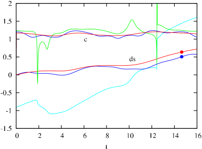
(a)                                           (b)

Figure 2: (Colour online) Visualisations of the relative periodic orbit $\textrm{RPO}_{M/14.646}$. (a) Phase speed $c=\dot{\ell}$ and deviation in shift $ds=\ell-\bar{c}t$ from a Galilean frame moving with mean phase speed $\bar{c}=1.11$: (green/cyan) ${{\hat{a}}^{\prime}}\equiv$$\mathrm{TW}_{1.85}$, (blue) template ${{\hat{a}}^{\prime}}$ on $\textrm{RPO}_{M/14.646}$, taken to be the state for which the wall friction is lowest, (red) method of connections.  (b) Three $\textrm{RPO}_{M/14.646}$ periods, starting from the large red dot, (blue) sliced with the template ${{\hat{a}}^{\prime}}$, and (red) method of connections, with times ${T}$, $2{T}$, $3{T}$ marked by the small red dot. The projection on ${a}_{i}=\langle{\hat{a}}|e_{i}\rangle$, where the $e_{i}$ are unit vectors (see main text).

3.1 Method of connections

If one were to use the state itself as a template at each instant in time, then a division by zero would always be avoided. This corresponds to projecting out the component parallel to the shift, i.e., the group orbit tangent, at each moment in time. In Rowley & Marsden (2000) this is referred to as the method of connections. While very appealing and sometimes deployed (Kreilos et al., 2014) to ‘calm’ a turbulent flow, the method of connections is not a symmetry reduction method, in the sense that the dimensionality of the state space is not reduced by 1 for each continuous symmetry parameter (see, e.g., Rowley et al. (2003); Cvitanović et al. (2012)). This is illustrated by figure 2. Starting with the same initial condition (fat red point), with the method of slices the orbit ${\hat{a}}(0)={\hat{a}}(T)$ closes after one period $T=14.646$ (blue), while with the method of connections the orbit continues filling out the relative periodic orbit torus ergodically, never closing into a periodic orbit. Figure 2 (b) shows a projection of the trajectory generated by the two approaches, for three cycles of the periodic orbit. Whereas the orbit closes for the method of slices, for the method of connections the invariant torus remains a torus. In conclusion, nothing is gained by using the method of connections.

The orthogonal unit vectors used in figure 2(b) are the leading components from a principal component analysis (PCA), using 586 symmetry-reduced states equi-spaced in time around the orbit. Further details are given in § 5.

3.2 First Fourier mode slice

The method of slices is local, and the slice border discontinuity is avoided only within a neighbourhood of the template. In our previous work (Willis et al., 2013), a switching approach was applied to help ensure closeness to the template. Whilst this enabled symmetry reduction of longer trajectories, it proved difficult to switch before reaching a border whilst simultaneously ensuring continuity of $\ell(t)$.

A different approach was taken by Budanur et al. (2015) for one-dimensional PDEs with $\textrm{SO}(2)$ symmetry, where it was shown that the first term in the Fourier expansion of the flow field can be used as the template for a global slice, border of which is never visited by generic ergodic trajectories. This method relied on the observation that projections of group orbits on the subspace spanned by the first Fourier mode components (sine and cosine) are non-overlapping circles; hence one can find a unique polar angle in this projection to quotient the $\textrm{SO}(2)$ symmetry. For a scalar field $u(x,t)=u(x+L,t)$ in one periodic space dimension, a slice template of the form $u^{\prime}=a\cos(2\pi x/L)+b\cos(2\pi x/L)$, where $a$ and $b$ are constants, defines a first Fourier mode slice. In higher dimensions, one has more freedom in choosing first Fourier mode slice templates. For pipe flow, any ${{\hat{a}}^{\prime}}$ corresponding to a velocity field of the form

$$\mbox{\boldmath$u$}^{\prime}(r,\theta,z)=\mbox{\boldmath$u$}_{c}(r,\theta)\cos(\alpha z)+\mbox{\boldmath$u$}_{s}(r,\theta)\sin(\alpha z)\,,$$ (17)

where $\mbox{\boldmath$u$}_{c,s}$ are three-dimensional vector fields that depend only on $r$ and $\theta$, can be a candidate for a first Fourier mode slice template. The vector fields $\mbox{\boldmath$u$}_{c,s}$ should be chosen such that the slice border condition $\langle{a}\vphantom{{{\hat{a}}^{\prime}}}|\vphantom{a}{{{\hat{a}}^{\prime}}}\rangle\,+\,\mathrm{i}\langle{a}\vphantom{g_{z}(L/4){{\hat{a}}^{\prime}}}|\vphantom{a}{g_{z}(L/4){{\hat{a}}^{\prime}}}\rangle=0$ is avoided by generic flow fields $\mbox{\boldmath$u$}=\mbox{\boldmath$u$}(r,\theta,z,t)$.

All slices are local, but since $\langle{g(-\ell)\,a}\vphantom{\mbox{\boldmath$t$}^{\prime}}|\vphantom{g(-\ell)\,a}{\mbox{\boldmath$t$}^{\prime}}\rangle=\langle{a}\vphantom{g(\ell)\,\mbox{\boldmath$t$}^{\prime}}|\vphantom{a}{g(\ell)\,\mbox{\boldmath$t$}^{\prime}}\rangle\,,$ one way to construct slice hyperplanes with larger domains of validity is by picking templates with smoother group orbits. Smoother states (i.e., states dominated by low Fourier modes) tend to be associated with lower dissipation or wall friction. Guided by this intuition, we construct the first Fourier mode slice template (17) by taking a low-dissipation solution from the turbulent set and setting all of its components to $0$ other than the ones with axial Fourier modes $k=1$ (Willis et al., 2016). For the calculation in figure 2, such a template was capable of capturing the whole orbit.

The slice-fixing shift $\ell(t)$ for a trajectory $a(t)$ is computed from the polar angle in the plane spanned by $({{\hat{a}}^{\prime}},g_{z}(L/4){{\hat{a}}^{\prime}})$ as

$$\ell(t)=\frac{L}{2\pi}\,\mbox{Arg}\left[\langle{a(t)}\vphantom{{{\hat{a}}^{\prime}}}|\vphantom{a(t)}{{{\hat{a}}^{\prime}}}\rangle+\mathrm{i}\langle{a(t)}\vphantom{g_{z}(L/4){{\hat{a}}^{\prime}}}|\vphantom{a(t)}{g_{z}(L/4){{\hat{a}}^{\prime}}}\rangle\right],$$ (18)

where Arg denotes the argument of the complex number. One can then find the translation symmetry-reduced trajectory $\hat{a}(t)$ by shifting the full state space trajectory $a(t)$ back to slice by $\hat{a}(t)=g_{z}(-\ell(t))a(t)\,.$

4 Invariant solutions

By carrying out an extensive search for travelling waves (6) and relative periodic orbits (7), we have found $8$ travelling waves and 48 relative periodic orbits of the pipe flow, listed in table 1. The travelling waves are labelled by their mean dissipation $\bar{D}$ (in units of the kinetic energy $E_{0}$ of the laminar solution), and relative periodic orbits by their periods $T$ (in units of $D/U$). The numerical method for finding most of these invariant solutions is the Newton–GMRES–hook iteration, discussed in detail in Viswanath (2007) and Chandler & Kerswell (2013). Relative periodic orbits with long periods tend to be more difficult (or impossible) to find with the standard Newton–GMRES–hook iteration. In order to capture such long orbits, we implemented a multiple-shooting Newton method, outlined in appendix A, and found $5$ relative periodic orbits, marked with subscript ‘M’ in table 1. The highly symmetric $N4$ type travelling wave of Pringle et al. (2009) belongs to an invariant subspace with an additional shift-and-rotate symmetry,

$$[u,v,w,p](r,\theta,z)=[u,-v,w,p](r,\theta-\pi/m_{0},z-L/2)\,.$$ (19)

The travelling waves $N4$ appear as a lower/upper branch pair and are therefore labeled as $N4L$ (lower branch) and $N4U$ (upper branch). The terminology refers to the appearance of these solutions from a saddle node bifurcation at a lower Re number as a pair of solutions with low ($N4L$) and high ($N4U$) dissipation rates. The lower branch solution is believed to belong to the laminar-turbulent boundary (Pringle et al., 2009).

Solution	$\bar{D}$	$\bar{c}$	$d_{U}$	$\mu^{\max}$	$\omega$ or $\theta$	Solution	$\bar{D}$	$\bar{c}$	$d_{U}$	$\mu^{\max}$	$\omega$ or $\theta$
$\textrm{TW}_{N4L/1.38}$‡	$1.38$	$1.238$	$3$	$0.1809$	$0.0$	$\textrm{TW}_{1.578}$	$1.578$	$1.108$	$9$	$0.2877$	$0.0$
$\textrm{TW}_{2.039}$‡	$2.039$	$1.091$	$7$	$0.1159$	$0.0$	$\textrm{TW}_{1.845}$	$1.845$	$1.039$	$11$	$0.5166$	$0.891$
$\textrm{TW}_{1.968}$‡	$1.968$	$1.105$	$9$	$0.1549$	$0.259$	$\textrm{TW}_{1.783}$	$1.783$	$1.035$	$8$	$0.323$	$1.119$
$\textrm{TW}_{1.885}$	$1.885$	$1.073$	$8$	$0.4568$	$0.206$	$\textrm{TW}_{2.041}$‡	$2.041$	$1.095$	$8$	$0.1608$	$0.0$
$\textrm{TW}_{N4U/3.28}$‡	$3.279$	$1.051$	$30$	$0.9932$	$1.89$	$\textrm{TW}_{1.926}$	$1.926$	$1.096$	$8$	$0.2504$	$0.414$
$\textrm{RPO}_{F/6.668}$‡	$1.805$	$1.12$	$3$	$0.0534$	$1.69$	$\textrm{RPO}_{F/M/33.81}$	$1.805$	$1.128$	$5$	$0.0471$	$1.727$
$\textrm{RPO}_{F/13.195}$‡	$1.839$	$1.117$	$5$	$0.0581$	$2.038$	$\textrm{RPO}_{F/33.968}$	$1.806$	$1.127$	$5$	$0.0588$	$1.671$
$\textrm{RPO}_{F/20.427}$‡	$1.809$	$1.128$	$5$	$0.0771$	$0.0$	$\textrm{RPO}_{F/40.609}$	$1.814$	$1.125$	$5$	$0.0505$	$0.315$
$\textrm{RPO}_{F/26.861}$	$1.84$	$1.121$	$5$	$0.0679$	$\pi$	$\textrm{RPO}_{F/M/47.449}$	$1.826$	$1.126$	$5$	$0.0586$	$\pi$
$\textrm{RPO}_{F/26.964}$	$1.826$	$1.124$	$6$	$0.0493$	$0.986$	$\textrm{RPO}_{F/M/53.876}$	$1.83$	$1.124$	$6$	$0.0457$	$1.253$
$\textrm{RPO}_{F/27.299}$‡	$1.815$	$1.126$	$4$	$0.0678$	$0.961$	$\textrm{RPO}_{F/M/67.936}$	$1.806$	$1.128$	$5$	$0.0587$	$2.945$
$\textrm{RPO}_{4.954}$‡	$2.015$	$1.084$	$3$	$0.1509$	$1.643$	$\textrm{RPO}_{M/14.544}$	$2.015$	$1.102$	$6$	$0.1846$	$0.0$
$\textrm{RPO}_{5.468}$	$2.003$	$1.091$	$6$	$0.1452$	$1.351$	$\textrm{RPO}_{M/14.646}$	$1.776$	$1.133$	$5$	$0.1473$	$\pi$
$\textrm{RPO}_{6.119}$	$1.875$	$1.081$	$7$	$0.1912$	$0.0$	$\textrm{RPO}_{14.961}$	$1.945$	$1.114$	$5$	$0.1915$	$0.878$
$\textrm{RPO}_{6.134}$	$1.86$	$1.086$	$7$	$0.1596$	$0.0$	$\textrm{RPO}_{15.081}$	$2.06$	$1.081$	$8$	$0.1392$	$0.0$
$\textrm{RPO}_{6.18}$	$1.865$	$1.091$	$5$	$0.211$	$0.0$	$\textrm{RPO}_{15.46}$‡	$1.781$	$1.146$	$7$	$0.1166$	$0.0$
$\textrm{RPO}_{6.359}$	$1.769$	$1.054$	$11$	$0.2614$	$0.0$	$\textrm{RPO}_{15.798}$	$1.869$	$1.125$	$6$	$0.1089$	$\pi$
$\textrm{RPO}_{6.458}$	$2.117$	$1.074$	$7$	$0.2055$	$0.0$	$\textrm{RPO}_{15.915}$	$1.951$	$1.106$	$8$	$0.1547$	$\pi$
$\textrm{RPO}_{7.246}$	$1.982$	$1.105$	$5$	$0.209$	$0.0$	$\textrm{RPO}_{15.972}$	$1.956$	$1.097$	$7$	$0.1473$	$\pi$
$\textrm{RPO}_{7.272}$	$2.015$	$1.1$	$5$	$0.1852$	$0.0$	$\textrm{RPO}_{16.271}$	$1.978$	$1.09$	$7$	$0.1454$	$1.977$
$\textrm{RPO}_{7.423}$‡	$1.838$	$1.109$	$6$	$0.1195$	$0.387$	$\textrm{RPO}_{16.878}$	$1.969$	$1.099$	$5$	$0.1219$	$\pi$
$\textrm{RPO}_{7.741}$‡	$1.707$	$1.138$	$5$	$0.0983$	$0.0$	$\textrm{RPO}_{17.21}$	$1.999$	$1.098$	$7$	$0.1523$	$\pi$
$\textrm{RPO}_{9.735}$‡	$2.05$	$1.086$	$7$	$0.1872$	$\pi$	$\textrm{RPO}_{17.46}$‡	$1.917$	$1.121$	$6$	$0.0842$	$0.205$
$\textrm{RPO}_{11.696}$	$1.961$	$1.108$	$9$	$0.1129$	$\pi$	$\textrm{RPO}_{21.704}$	$1.868$	$1.12$	$7$	$0.0951$	$\pi$
$\textrm{RPO}_{12.026}$	$2.09$	$1.088$	$6$	$0.1476$	$0.0$	$\textrm{RPO}_{22.063}$	$2.032$	$1.101$	$7$	$0.1352$	$1.723$
$\textrm{RPO}_{12.566}$	$2.053$	$1.083$	$10$	$0.1677$	$\pi$	$\textrm{RPO}_{23.047}$	$1.874$	$1.12$	$6$	$0.1848$	$0.0$
$\textrm{RPO}_{12.706}$	$2.156$	$1.07$	$6$	$0.1692$	$1.083$	$\textrm{RPO}_{23.356}$‡	$1.98$	$1.112$	$6$	$0.101$	$1.249$
$\textrm{RPO}_{13.592}$	$1.987$	$1.099$	$7$	$0.1072$	$0.0$	$\textrm{RPO}_{26.049}$	$2.028$	$1.097$	$8$	$0.1635$	$\pi$
$\textrm{RPO}_{14.045}$‡	$1.903$	$1.107$	$6$	$0.1403$	$\pi$	$\textrm{RPO}_{27.238}$	$1.992$	$1.098$	$8$	$0.1258$	$0.0$

Table 1: The list of the invariant solutions reported in this work. Average rate of dissipation $\bar{D}$, average down-stream phase velocity $\bar{c}$, dimension of the unstable manifold $d_{U}$, real part of the largest stability eigenvalue / Floquet exponent $\mu^{max}$ is shown. Last column corresponds to the imaginary part $\omega$ of the leading stability eigenvalue for travelling waves, and phase $\theta$ of the leading Floquet multiplier for relative periodic orbits. Travelling waves are labeled by their dissipation rate $\bar{D}$, relative periodic orbits by their period ${T}$. A family of twelve relative periodic orbits which appear to have similar physical properties are grouped together and labeled with subscript $F$. Solutions marked with ‡  were previously reported in Table 1 of Willis et al. (2016). The six solutions marked with $M$ were obtained by the multiple-shooting Newton method of appendix A.

The travelling waves linear stability exponents $\lambda_{j}=\mu_{j}+i\omega_{j}$ are computed by linearizing the governing equations in the co-moving frame, in which a travelling wave becomes an equilibrium. The leading stability exponent, i.e., the exponent with the largest real part, is reported in table 1. The integer $d_{U}$ denotes the number of exponents with positive real parts, $\mu_{j}>0$, which determine the dimension of the unstable manifold of the travelling wave.

The linear stability of a relative periodic orbit is described by its Floquet multipliers $\Lambda_{j}=\exp(\mu_{j}T+i\theta_{j})$. As for the travelling waves, in table 1 we report the number of the unstable directions $d_{U}$, real part $\mu^{max}$ of the leading Floquet exponent $\lambda_{j}=(1/T)\ln|\Lambda_{j}|$, and the phase $\theta$ of the leading Floquet multiplier of the relative periodic orbit.

Twelve relative periodic orbits listed in table 1 (indicated by subscript $F$) are separated from the rest in the table. We refer to these orbits as the first family solutions, due to their remarkably similar physical and dynamical properties. The periods of the first family members are approximately integer multiples of the shortest relative periodic orbit, whose period is ${T}=6.668$. Indeed, numerical continuations in $Re$ and/or geometry parameters show that several first family members originated from bifurcations off the parent orbit $\textrm{RPO}_{F/6.668}$. For example, $\textrm{RPO}_{F/13.195}$ is born out of a period-doubling bifurcation at $Re=2191$. As is shown in the next section, the first family orbits lie near each other in all state space visualisations, populating a small region of the state space. A detailed bifurcation analysis of the first family orbits is the subject of ongoing research (Short & Willis, 2017).

5 State-space visualisation of fluid flows

With the available computational resources, today one can generate a large number of turbulent trajectories as solutions of the Navier–Stokes equations with various initial conditions. What can one learn from the resulting enormous amounts of data?

A routine approach is to seek to understand the statistical properties of physically relevant quantities such as velocity correlations, enstrophy, palinstrophy, etc. One objective of the program of determining invariant solutions is to go beyond a statistical description, and explore the state space geometry of long-time attractors of such dissipative flows. This should ultimately provide a coarse-grained partition of the state space into regions of qualitatively and quantitatively similar behaviours.

Embarking on this path, one is immediately confronted with several fundamental dilemmas with no known resolution:

1. State space geometry. Inertial manifolds and attracting sets of nonlinear dissipative flows are nonlinear, curved subsets of the full state space. Even for the Hénon attractor we only have a partial understanding of the topology (Cvitanović et al., 1988; de Carvalho & Hall, 2002) and the existence of such attracting sets (Benedicks & Carleson, 1991). Our strategy for visualisation of the ‘state space geometry’ of the Navier–Stokes equations is to populate it by invariant solutions, e.g. equilibria, travelling waves, periodic orbits and relative periodic orbits, and capture the local “curvature” of the attractor by tracing out segments of their unstable manifolds and their heteroclinic connections (see, e.g., Gibson et al. (2008); Halcrow et al. (2009))

2. Measuring distances. The distance between two fluid states is measured using some norm. There is no solid physical or mathematical justification for using the usual $L_{2}$ or ‘energy’ norm. For example, in some problems a Sobolev norm might be preferred in order to either penalize or emphasize the small scale structures (see, e.g., Mathew et al. (2007); Lin et al. (2011); Farazmand (2016) and § 5.4). Furthermore, in presence of continuous and discrete symmetries, it is absolutely imperative that symmetries be reduced before a distance can be measured (see, e.g., (35)); states on group orbits of nearby states can lie arbitrarily far in the state space. As different choices of a slice yield different distances, this introduces a further arbitrariness into the notion of ‘distance’.

3. Low-dimensional visualisations. The state space of Navier–Stokes equations is infinite-dimensional. To visualize the geometry of the invariant solutions one inevitably projects the solutions to two- or three-dimensional subspaces. For a discussion of optimal projections that best illuminate the structure of an attractor, see Cvitanović (2017).

Although we are in no position to resolve any of these issues in this paper, we will elucidate, through examples, the impact of the choice one makes in answering each question.

5.1 Choice of the norm

In this work, we use two rather different norms, the standard energy norm, and a hand-crafted ‘low pass’ norm. In what follows, we show how the choice of the norm can significantly alter the state space visualisations, and the conclusions drawn from them.

Let $\mbox{\boldmath$u$}=\sum_{km}\mbox{\boldmath$u$}_{km}(r)\exp(2\mathrm{i}\alpha kz+\mathrm{i}m_{0}m\theta)$ denote the Fourier series of a velocity field $u$ defined in a pipe of axial length $L=\pi/\alpha$. The variables $\mbox{\boldmath$u$}_{km}$ denote the Fourier coefficients corresponding to the axial and azimuthal directions as functions of the radial distance $r$. For two velocity fields $\mbox{\boldmath$u$}_{1}$ and $\mbox{\boldmath$u$}_{2}$, we define the $L^{2}$ inner product

$$\langle{\mbox{\boldmath$u$}_{1}}\vphantom{\mbox{\boldmath$u$}_{2}}|\vphantom{\mbox{\boldmath$u$}_{1}}{\mbox{\boldmath$u$}_{2}}\rangle_{L^{2}} = \frac{1}{2E_{\mathrm{HP}}}\int_{V}\mbox{\boldmath$u$}_{1}\cdot\mbox{\boldmath$u$}_{2}\,r\,d\theta\,dr\,dz\,,$$ (20)

$$= \frac{1}{E_{\mathrm{HP}}}\int_{0}^{1/2}\!\!r\,dr\,\sum_{k,m}\mbox{\boldmath$u$}^{*}_{1,km}(r)\cdot\mbox{\boldmath$u$}_{2,km}(r)\,,$$ (21)

where $V$ denotes the cylindrical flow domain and $E_{\mathrm{HP}}$ is the kinetic energy of the Hagen-Poiseuille flow. In (21), we write the integral explicitly in terms of Fourier modes and radial integration, which in practice are approximated numerically. This inner product corresponds to the $L^{2}$ or the kinetic energy norm,

$$E(\mbox{\boldmath$u$})=\frac{1}{2}\left\|\mbox{\boldmath$u$}\right\|_{L^{2}}^{2}=\frac{1}{2}\langle{\mbox{\boldmath$u$}}\vphantom{\mbox{\boldmath$u$}}|\vphantom{\mbox{\boldmath$u$}}{\mbox{\boldmath$u$}}\rangle_{L^{2}}.$$ (22)

We sometimes find it more informative to use a metric that emphasizes larger scale structures along the continuous symmetry directions. For this reason, we define the ‘low pass’ metric,

$$\langle{\mbox{\boldmath$u$}_{1}}\vphantom{\mbox{\boldmath$u$}_{2}}|\vphantom{\mbox{\boldmath$u$}_{1}}{\mbox{\boldmath$u$}_{2}}\rangle_{LP}=\frac{1}{V}\int_{0}^{1/2}rdr\sum_{k,m}\frac{1}{1+(\alpha k)^{2}+(m_{0}m)^{2}}\,\mbox{\boldmath$u$}^{*}_{1,km}(r)\cdot\mbox{\boldmath$u$}_{2,km}(r)\,,$$ (23)

which penalizes higher Fourier modes (short wavelengths. In the axial and azimuthal directions this is a variation of a Sobolev $H^{-1}$ norm (Lax, 2002): The weights are smaller for larger values of $k$ and $m$, hence shorter wavelengths are de-emphasized.

In the work reported here, we rely primarily on the energy norm (21), except for § 5.4 where we contrast state space visualisations using the energy and the low pass norms, and comment on their relative effectiveness in our searches for relative periodic orbits.

5.2 Global visualisations: Principal Component Analysis

We begin our investigation of state space with a data-driven method in order to obtain a general qualitative picture. The use of principal component analysis (PCA), otherwise known as proper orthogonal decomposition (POD) in the context of fluids, has been well documented (see e.g. Berkooz et al. (1993)). Broadly speaking, the method extracts a set of orthogonal vectors that span the data with minimal residual, with respect to some norm.

Here we apply the method to extract principal components, relative to the mean $\bar{{\hat{a}}}$ of the data set of $N$ states ${\hat{a}}_{i}$ in the symmetry-reduced state space, symmetrized with respect to $g_{\theta}$. Singular value decomposition is applied to the matrix of inner products of the deviations $\tilde{{\hat{a}}}_{i}={\hat{a}}_{i}-\bar{{\hat{a}}}$,

$$R_{ij}=\frac{1}{N-1}\langle{\tilde{{\hat{a}}}_{i}}\vphantom{\tilde{{\hat{a}}}_{j}}|\vphantom{\tilde{{\hat{a}}}_{i}}{\tilde{{\hat{a}}}_{j}}\rangle_{\mathrm{L^{2}}}\,,\qquad R=U\,S\,V^{T}\,,$$ (24)

from which the $j^{\mathrm{th}}$ principal component is calculated

$$\mbox{\boldmath$e$}_{j}=\sum_{i=1}^{N}\tilde{{\hat{a}}}_{j}U_{ij}\,,\qquad\hat{\mbox{\boldmath$e$}}_{j}=\mbox{\boldmath$e$}_{j}/\langle{{\mbox{\boldmath$e$}}_{j}}\vphantom{{\mbox{\boldmath$e$}}_{j}}|\vphantom{{\mbox{\boldmath$e$}}_{j}}{{\mbox{\boldmath$e$}}_{j}}\rangle_{\mathrm{L^{2}}}\,.$$ (25)

Each principal component $\hat{\mbox{\boldmath$e$}}_{j}$ has the property that the root-mean-square of the projection $p_{j}=\langle{\tilde{{\hat{a}}}_{i}(t)}\vphantom{\hat{\mbox{\boldmath$e$}}_{j}}|\vphantom{\tilde{{\hat{a}}}_{i}(t)}{\hat{\mbox{\boldmath$e$}}_{j}}\rangle$ (taking the mean over $i$) equals the $j^{\mathrm{th}}$ singular value, $S_{jj}$, of the correlation matrix.

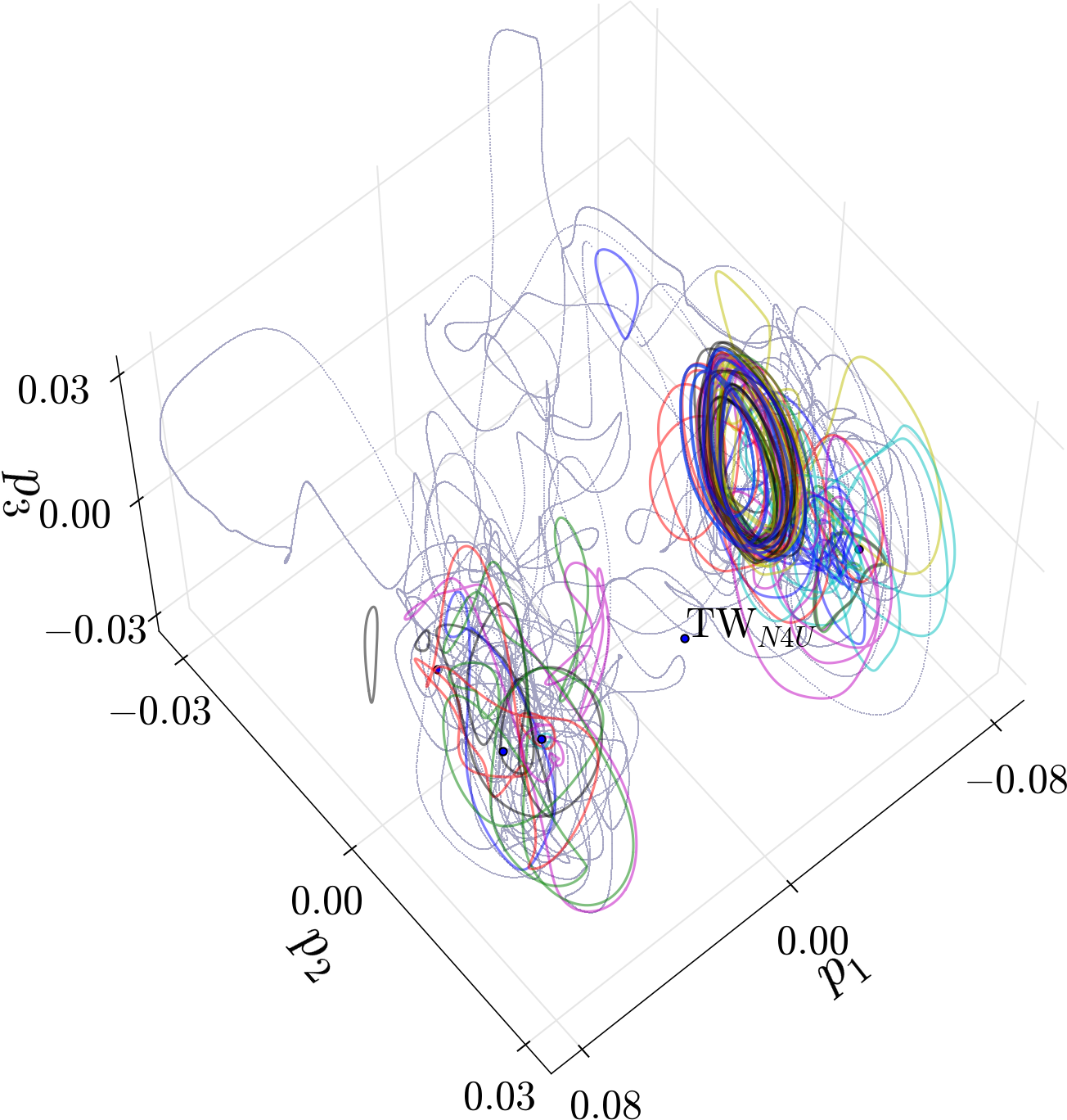
(a) (b)

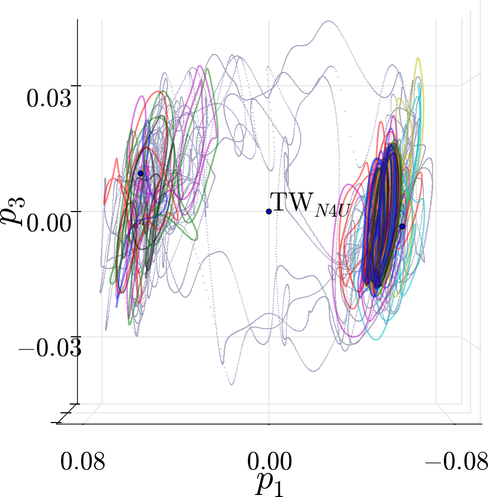
Figure 3: (Colour online) Relative periodic orbits (closed curves, different colors), $5$ travelling waves (marked with black dots), and an two turbulent trajectories (gray, transparent dots) of the pipe flow projected onto first three principal components (25), two different viewing angles.

Principal components were extracted from $2000$ uncorrelated symmetry-reduced states obtained from ergodic trajectories. Figure 3 shows all our relative periodic orbits, $5$ travelling waves, and two turbulent trajectories projected onto the principal components, computed as above. There are some notable observations about figure 3: Firstly, periodic orbits appear to be localized on two sides of the $p_{1}=0$ plane, and the turbulent trajectories rarely switch from one side to other. The first Fourier mode slice reduces the continuous translation symmetry of pipe flow but the discrete half-rotation symmetry $g_{\theta}$ still remains; the two sides of figure 3 are related to each other by this discrete symmetry operation. Also note that the highly symmetric $N4$ travelling wave $\textrm{TW}_{N4U/3.28}$, which is invariant under $g_{\theta}$, appears to lie at the origin of $(p_{1},p_{3})$ plane.

It is clear from figure 3 that the principal component $\hat{\mbox{\boldmath$e$}}^{\prime}_{1}$ is aligned along the symmetry direction. This makes the information contained along this direction redundant, since each solution with $p_{1}>0$ has a copy with $p_{1}<0$. As we are most interested in the details of the turbulent set and invariant dynamical behaviour of the system, our next step is to reduce the discrete $g_{\theta}$-symmetry. For this purpose, we define the ‘fundamental domain’ (Cvitanović et al., 2017) as $p_{1}>0$ and bring all our data from turbulence simulations and invariant solutions to this half of the state space. With the desymmetrized turbulence data, we recompute principal components $\tilde{\mbox{\boldmath$e$}}^{\prime}_{j}$, which we will refer to as ‘fundamental domain principal components’.

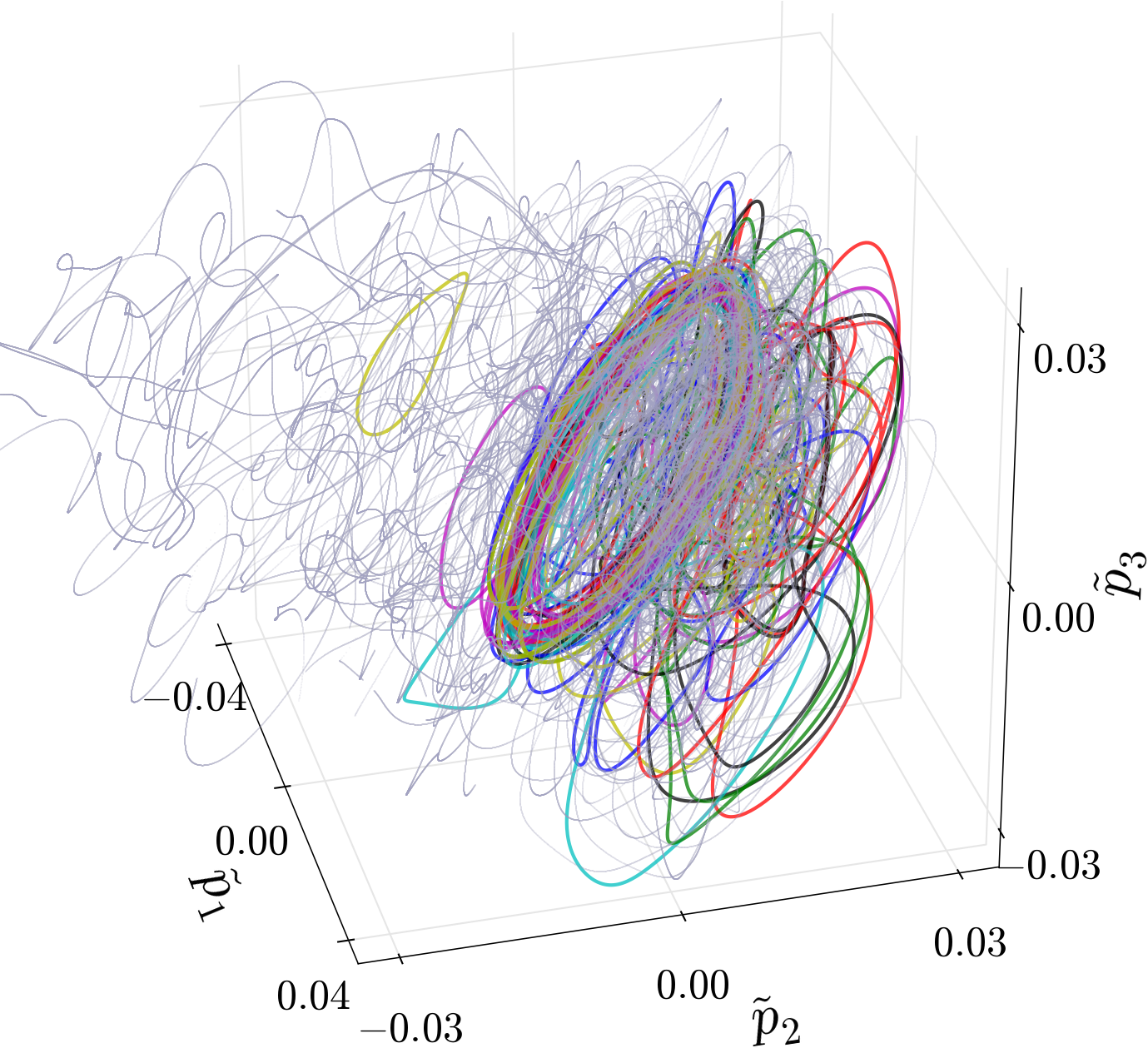
(a) (b)

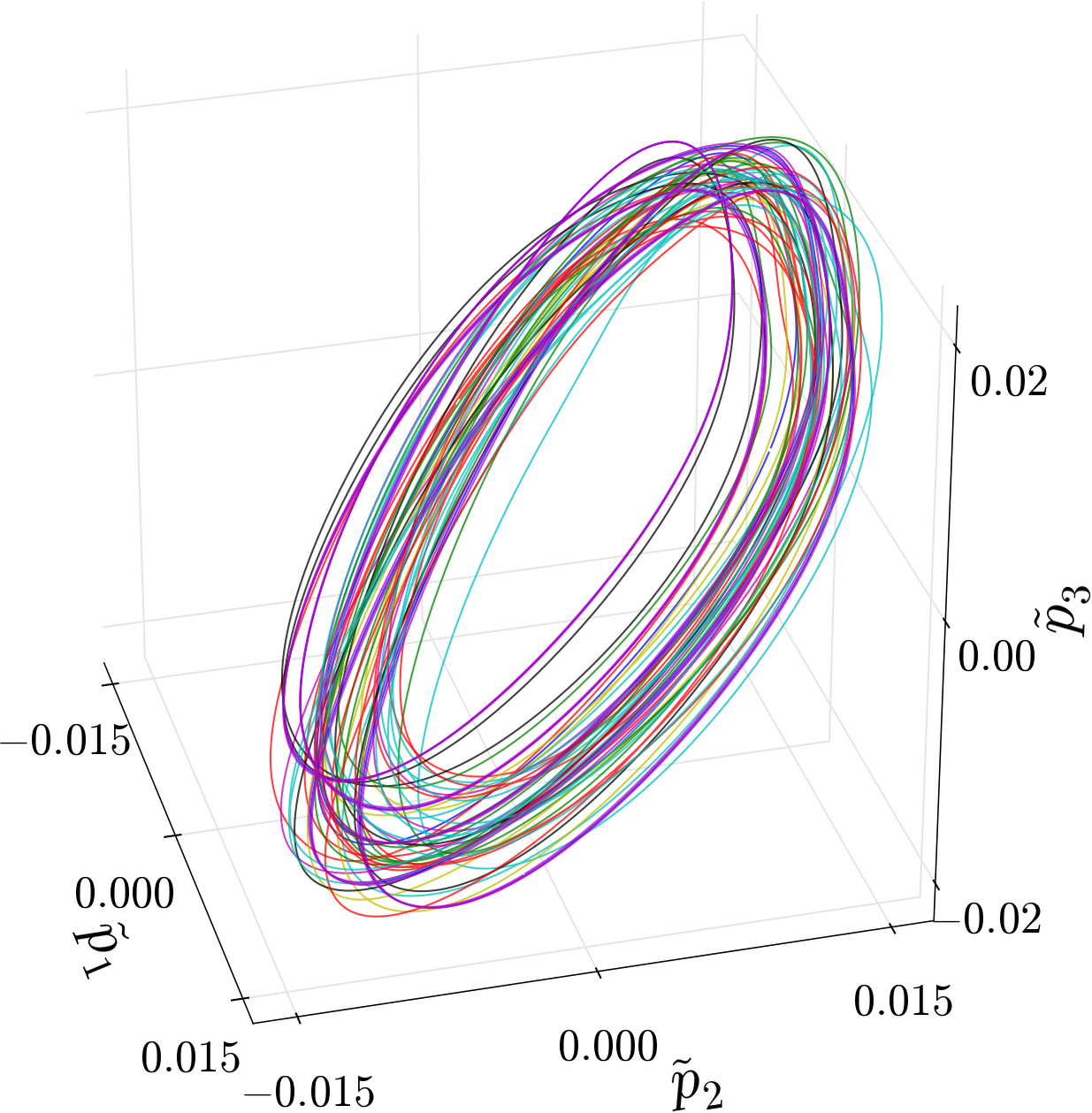
Figure 4: (Colour online) (a) Relative periodic orbits (closed curves of various colors) and 5 turbulent trajectories (gray dots) projected onto first three fundamental domain principal components. (b) $11$ orbits, which appear to fill out a region of the state space.

Figure 4 shows relative periodic orbits and turbulent trajectories projected onto the three dominant fundamental domain principal components. In figure 4, we no longer have two “clouds” and relative periodic orbits are mostly located in the region of state space where turbulent trajectories spend most of their time. One striking observation from figure 4 (a) is that a subset of relative periodic orbits seem to be located close to one another and their projections also qualitatively resemble each other. These are the relative periodic orbits labelled with subscript F in table 1. We have already noted that the periods of these relative periodic orbits are approximately integer multiples of the shortest one. Their qualitative similarities in the state space projections of figure 4 provide further evidence that these orbits are related to one another, possibly through sequences of bifurcations at other values of the Re number (Short & Willis, 2017).

In order to develop more intuition about the state space geometry, we reduce the flow further to a Poincaré section defined by

$$\langle{\tilde{a}_{\cal P}-\left\langle{\tilde{a}}\right\rangle}\vphantom{\tilde{\mbox{\boldmath$e$}}^{\prime}_{3}}|\vphantom{\tilde{a}_{\cal P}-\left\langle{\tilde{a}}\right\rangle}{\tilde{\mbox{\boldmath$e$}}^{\prime}_{3}}\rangle_{L^{2}}=0\,,\quad\langle{\hat{v}(\tilde{a}_{\cal P})}\vphantom{\tilde{\mbox{\boldmath$e$}}^{\prime}_{3}}|\vphantom{\hat{v}(\tilde{a}_{\cal P})}{\tilde{\mbox{\boldmath$e$}}^{\prime}_{3}}\rangle_{L^{2}}>0\,.$$ (26)

In the projections of figure 4, the Poincaré section (26) corresponds to $\tilde{p}_{3}=0$ plane, and for visualisations of figure 5, we project intersections onto the $(\tilde{\mbox{\boldmath$e$}}^{\prime}_{1},\tilde{\mbox{\boldmath$e$}}^{\prime}_{2})$ plane. However, it should be noted that this Poincaré section is a codimension-1 hyperplane in the symmetry reduced state space. Figure 5 (a) shows $8560$ intersections (grey) of turbulent trajectories with the Poincaré section (26) that were obtained from $147$ individual runs, along with those (red and green) of relative periodic orbits.

It is clear in figure 5 (a) that the turbulence visits the region containing relative periodic orbits more often than the rest of the state space. In figure 5, the ‘first family’ of relative periodic orbits shown in figure 4 are marked red, except for $\textrm{RPO}_{F/6.668}$, the shortest one, which is colored black. Figure 5 (b) is a close-up view of the region containing relative periodic orbits, enclosed by the dashed-rectangle in figure 5 (a) and similarly, figure 5 (c) is a close-up of the region containing the first family, marked with the dashed rectangle on figure 5 (b). In figure 5 (d), we show orbits which approximate the three-dimensional unstable manifold of $\textrm{RPO}_{F/6.668}$ overlaid over figure 5 (c). (The computational aspects of tracing out the unstable manifold are discussed in § 5.3.)

\begin{overpic}[width=195.12767pt]{psectwPOs} \put(0.0,0.0){(a)} \end{overpic}

\begin{overpic}[width=195.12767pt]{psectZoomwPOs} \put(0.0,0.0){(b)} \end{overpic}

\begin{overpic}[width=195.12767pt]{psectZzoomwPOs} \put(0.0,0.0){(c)} \end{overpic}

\begin{overpic}[width=195.12767pt]{psectZzoomwUnstMan} \put(0.0,0.0){(d)} \end{overpic}

Figure 5: (Colour online) (a) Turbulent trajectories (grey), and relative periodic orbits (black: $\textrm{RPO}_{F/6.668}$, red: other members of the first family, green: the rest) on the Poincaré section (26). (b) Zoom-into the region enclosed by the dashed-rectangle on (a). (c) Zoom-into the region enclosed by the dashed-rectangle on (b). (d) Trajectories (cyan) on the unstable manifold of $\textrm{RPO}_{F/6.668}$ added to (c).

The global visualisations of dynamics we presented above provide us with insights about the state space structure: the most important observation is that turbulent dynamics frequently visits the neighbourhoods of the relative periodic orbits found in this work. In addition, the “first family” orbits—the set sharing similar physical and stability properties—appear close to each other in all projections of figure 4 and figure 5. Furthermore, the unstable manifold of the shortest period member of this family visits the intersections of the other members of the family on figure 4, which provides additional evidence that these orbits emerge from a common bifurcation sequence (Short & Willis, 2017).

Note that in the zoomed-in projection of the Poincaré section, figure 5 (c), some parts are often visited by the turbulent trajectories (as indicated by the overlapping markers), while there are other regions, even the ones that appear close to the frequently visited regions, that tend to remain empty. This illustrates why measuring distances in the state space of a turbulent fluid is a hard problem: Two points in state space that are seemingly very close to each other in $L_{2}$ or a similar norm may be completely separated dynamically, since the geometry of the manifold on which the turbulence takes place can be highly convoluted.

While the global visualisations give us a qualitative view of the state space, they cannot tell us much about the finer structure of the turbulent state space. This is not surprising since the state space in question is very high dimensional; and it is very unlikely that we can obtain a complete picture of dynamics from two- and three-dimensional global visualisations. For a better understanding of the state space geometry, one must study the neighbourhoods of important invariant solutions individually, as illustrated in the next section.

5.3 Local visualisations

Global visualisations of the state space in figures 4 and 5 support the earlier suggestion that the members of the first family of relative periodic orbits, embedded in turbulence and listed separately in table 1, may be dynamically related to each other. The shortest period member $\textrm{RPO}_{F/6.668}$ of first family has three unstable ($|\Lambda_{i}|>1$) Floquet multipliers:

$$\Lambda_{1,2}=-0.1698\pm i1.418\,,\quad\Lambda_{3}=-1.340\,.$$ (27)

This renders the associated unstable manifold of $\textrm{RPO}_{F/6.668}$ three-dimensional even after the symmetry reduction of the space and time translation directions. Leading complex conjugate Floquet multipliers imply spiral-out dynamics in the associated neighbourhood, while the negative-real third Floquet multiplier implies that locally there exists a topologically Möbius band-shaped dynamics such as the one observes in period-doubling bifurcations. In the following, we numerically approximate and visualize these one- and two-dimensional unstable sub-manifolds.

Budanur & Cvitanović (2015) numerically approximated the one- and two-dimensional unstable manifolds of relative periodic orbits in a Kuramoto–Sivashinsky system. In those computations, a local Poincaré section was constructed in the neighbourhood of a periodic orbit where they initiated orbits whose dynamics approximately covered the linear unstable manifold; hence their forward integration approximated the unstable manifold away from the linearized neighbourhood. This strategy was adapted for calculating one-dimensional unstable manifold of the localized “edge state” relative periodic orbit of the pipe flow in Budanur & Hof (2017), in order. We apply here this method to a relative periodic orbit embedded in turbulence, with a three-dimensional unstable manifold, a case that was not considered in the aforementioned studies.

To this end, we first define a local Poincaré section in the neighbourhood of $\textrm{RPO}_{F/6.668}$ as the half-hyperplane

$$\langle{{\hat{a}}_{\cal P}-{\hat{a}}_{p}}\vphantom{\hat{v}({\hat{a}}_{p})}|\vphantom{{\hat{a}}_{\cal P}-{\hat{a}}_{p}}{\hat{v}({\hat{a}}_{p})}\rangle_{L^{2}}=0\,,\quad\langle{\hat{v}({\hat{a}}_{\cal P})}\vphantom{\hat{v}({\hat{a}}_{p})}|\vphantom{\hat{v}({\hat{a}}_{\cal P})}{\hat{v}({\hat{a}}_{p})}\rangle_{L^{2}}>0\,,$$ (28)

where ${\hat{a}}_{p}$ is a point on $\textrm{RPO}_{F/6.668}$, which we have arbitrarily chosen as its intersection with the global Poincaré section (26). The relative periodic orbit $\textrm{RPO}_{F/6.668}$ is a fixed point of the Poincaré map on the section (28) with stability multipliers equal to its Floquet multipliers. Associated Floquet vectors, however, need to be projected onto this section. This is a two-stage process since we compute the Floquet vectors as eigenfunctions $V_{i}$ of the eigenvalue problem

$$g_{z}(-l_{p})\frac{d{f^{{T_{p}}}(\mbox{\boldmath$\hat{u}$}_{p})}}{d\mbox{\boldmath$\hat{u}$}_{p}}V_{i}=\Lambda_{i}V_{i}\,,$$ (29)

in full state space. First we project these vectors onto the slice as

$$\hat{V}_{i}=V_{i}-\frac{\langle{\mathbf{t}{}^{\prime}}\vphantom{V_{i}}|\vphantom{\mathbf{t}{}^{\prime}}{V_{i}}\rangle_{L^{2}}}{\langle{\mathbf{t}({\hat{a}}_{p})}\vphantom{\mathbf{t}{}^{\prime}}|\vphantom{\mathbf{t}({\hat{a}}_{p})}{\mathbf{t}{}^{\prime}}\rangle_{L^{2}}}\mathbf{t}({\hat{a}}_{p}),$$ (30)

where $\hat{V}_{i}$ denotes the projected vector on the slice. Then we project translation-symmetry reduced Floquet vectors onto the Poincaré section as

$$\hat{V}_{i,{\cal P}}=\hat{V}_{i}-\frac{\langle{\hat{v}({\hat{a}}_{p})}\vphantom{\hat{V}_{i}}|\vphantom{\hat{v}({\hat{a}}_{p})}{\hat{V}_{i}}\rangle_{L^{2}}}{\langle{\hat{v}({\hat{a}}_{p})}\vphantom{\hat{v}({\hat{a}}_{p})}|\vphantom{\hat{v}({\hat{a}}_{p})}{\hat{v}({\hat{a}}_{p})}\rangle_{L^{2}}}\hat{v}({\hat{a}}_{p})\,.$$ (31)

Projections (30) and (31) onto slice hyperplane (14) and onto the Poincaré section hyperplane (28) follow the same geometrical principle as the Appendix of (Budanur & Hof, 2017).

In order to visualise the one-dimensional unstable submanifold of $\textrm{RPO}_{F/6.668}$, we initiate trajectories from the points

$${\hat{a}}_{\cal P}(\delta)={\hat{a}}_{p}\pm\epsilon|\Lambda_{3}|^{\delta}\hat{V}_{3,{\cal P}}\,,\quad\mbox{where}\quad\delta\in[0,1)\,.$$ (32)

These initial conditions approximately cover the locally linear one-dimensional piece of the unstable manifold in $\hat{V}_{3,{\cal P}}$ direction such that first-return of $\tilde{a}_{\cal P}(0)$ coincides with initial location of $\tilde{a}_{\cal P}(1)$. We discretised (32) by choosing four equidistant points in $\delta$ and set $\epsilon=10^{-3}$ (Floquet vectors are normalized such that $\left\|a_{p}\right\|_{L^{2}}=\left\|V_{i}\right\|_{L^{2}}$). We forward-integrate these initial conditions while recording their intersections with the Poincaré section (28). Figure 6 (a,b) shows the first $25$ intersections of these orbits with the Poincaré section on two-dimensional projections and panels (c,d) shows one of these orbits in a three-dimensional projection along with $\textrm{RPO}_{F/6.668}$ and $\textrm{RPO}_{F/13.195}$. The origin of the projections in figure 6 is ${\hat{a}}_{p}$ and the projection coordinates are

$$e_{1} = \langle{{\hat{a}}}\vphantom{{\rm Re\,}\hat{V}_{1,\bot}}|\vphantom{{\hat{a}}}{{\rm Re\,}\hat{V}_{1,\bot}}\rangle_{L^{2}}\,,\quad e_{2}\,=\,\langle{{\hat{a}}}\vphantom{{\rm Im\,}\hat{V}_{1,\bot}}|\vphantom{{\hat{a}}}{{\rm Im\,}\hat{V}_{1,\bot}}\rangle_{L^{2}},$$

$$e_{3} = \langle{{\hat{a}}}\vphantom{\hat{V}_{3,\bot}}|\vphantom{{\hat{a}}}{\hat{V}_{3,\bot}}\rangle_{L^{2}}\,,\qquad e_{4}\,=\,\langle{{\hat{a}}}\vphantom{\hat{V}_{6,\bot}}|\vphantom{{\hat{a}}}{\hat{V}_{6,\bot}}\rangle_{L^{2}},$$ (33)

$$e_{5} = \langle{{\hat{a}}}\vphantom{\hat{v}({\hat{a}}_{p})/\left\|\hat{v}({\hat{a}}_{p})\right\|_{L^{2}}}|\vphantom{{\hat{a}}}{\hat{v}({\hat{a}}_{p})/\left\|\hat{v}({\hat{a}}_{p})\right\|_{L^{2}}}\rangle_{L^{2}},$$

where $\hat{V}_{6,\bot}$ is the symmetry-reduced Floquet vector in the least stable direction (comes after marginal axial and temporal translation directions), and subscript $\bot$ indicates that these vectors are Gram-Schmidt orthonormalized.

\begin{overpic}[width=195.12767pt]{Con2D2} \put(0.0,0.0){(a)} \end{overpic}

\begin{overpic}[width=195.12767pt]{Con2D1} \put(0.0,0.0){(b)} \end{overpic}

\begin{overpic}[width=195.12767pt]{Con3D1} \put(0.0,0.0){(c)} \end{overpic}

\begin{overpic}[width=195.12767pt]{Con3D2} \put(0.0,0.0){(d)} \end{overpic}

Figure 6: (Colour online) (a,b) One-dimensional submanifold in the unstable manifold of $\textrm{RPO}_{F/6.668}$ capturing locally linear dynamics in the $\hat{V}_{3,{\cal P}}$ direction in the Poincaré section, two projections onto local coordinates (33). Fixed point corresponding to $\textrm{RPO}_{F/6.668}$ is at the origin (red), and the 2-cycle $\textrm{RPO}_{F/13.195}$ is marked blue. (c,d) Three-dimensional projections of one ($\delta=0$) of the $8$ trajectories in panels (a,b).

Figure 6 (a,b) shows that one-dimensional shape of locally linear dynamics is preserved as it is extended far away from the origin. Trajectories in figure 6 (a,b) spread in a higher-dimensional manifold once they reach the neighbourhood of period-doubled $\textrm{RPO}_{F/13.195}$. For additional comparison, in figure 6 (c,d) we plot different three-dimensional projections of $\textrm{RPO}_{F/6.668}$, the $\delta=0$ in (32) orbit, and $\textrm{RPO}_{F/13.195}$ in different three-dimensional projections. Qualitative similarities between the shape of the unstable manifold and $\textrm{RPO}_{F/13.195}$ are remarkable. For a quantitative conclusion, one should search for a heteroclinic connection from three-dimensional unstable manifold of $\textrm{RPO}_{F/6.668}$ to the relative periodic orbit $\textrm{RPO}_{F/13.195}$. That, however, is beyond the scope of the current work.

For further comparison, we visualise the streamwise velocity and vorticity isosurfaces of $\textrm{RPO}_{F/6.668}$, $\textrm{RPO}_{F/13.195}$, and three-snapshots on the unstable manifold of $\textrm{RPO}_{F/6.668}$ in figure 7. All panels of figure 7 correspond to their respective intersections with the Poincaré section (28), and only one-eighth (one-quarter in azimuthal and one-half in axial directions) of the pipe is shown. The one-eighth visualisation suffices, since we work in the subspace with 4-fold symmetry in the azimuthal direction, and the other half of the pipe in the axial direction can be obtained from the first half by the shift-and-reflect (4) symmetry.

While all panels of figure 7 appear similar, they differ in details. Figure 7 (d), the initial point on the unstable manifold, is virtually indistinguishable from $\textrm{RPO}_{F/6.668}$ in figure 7 (a). Flow structures of $\textrm{RPO}_{F/13.195}$ at its two-intersections with the Poincaré section, figure 7 (b,c), differ from $\textrm{RPO}_{F/6.668}$ and from each-other only in minute details; one has to compare the streak and roll sizes one-by-one. These nuances are reflected on the selected points on the unstable manifold shown in figure 7 (d,e,f), although only identifiable after a careful inspection. These difficulties illustrate the power of state space visualisation (cf. figure 6), without which the relation of $\textrm{RPO}_{F/6.668}$ to $\textrm{RPO}_{F/13.195}$ would have been very hard to elucidate.

\begin{overpic}[width=130.08731pt]{66699000} \put(0.0,0.0){(a)} \end{overpic}

\begin{overpic}[width=130.08731pt]{66529000} \put(0.0,0.0){(b)} \end{overpic}

\begin{overpic}[width=130.08731pt]{66529001} \put(0.0,0.0){(c)} \end{overpic}

\begin{overpic}[width=130.08731pt]{man09000} \put(0.0,0.0){(d)} \end{overpic}

\begin{overpic}[width=130.08731pt]{man09023} \put(0.0,0.0){(e)} \end{overpic}

\begin{overpic}[width=130.08731pt]{man09024} \put(0.0,0.0){(f)} \end{overpic}

Figure 7: (Colour online) Streamwise velocity isosurfaces at $u=\pm 0.5U_{b}$ (red and blue) and streamwise vorticity isosurfaces at $\omega_{z}=\pm 2.4(U_{b}/D)$ (purple and green) of (a) $\textrm{RPO}_{F/6.668}$; (b,c) $\textrm{RPO}_{F/13.195}$; and (d,e,f) the unstable manifold of $\textrm{RPO}_{F/6.668}$ at discrete times $n=0,23,24$.

A set of initial conditions that approximately covers the linearised dynamics in the plane $({\rm Re\,}\hat{V}_{1,{\cal P}},{\rm Im\,}\hat{V}_{1,{\cal P}})$ is given by

$$\tilde{a}_{\cal P}(\phi,\delta)=\hat{a}_{p}\pm\epsilon|\Lambda_{1}|^{\delta}({\rm Re\,}\hat{V}_{1,{\cal P}}\cos\phi+{\rm Im\,}\hat{V}_{1,{\cal P}}\sin\phi)\,,\quad\delta\in[0,1)\,,\quad\phi\in[0,2\pi).$$ (34)

We discretise (34) by choosing $4$ equidistant points in $\delta$ and $36$ points in $\phi$ and set $\epsilon=10^{-3}$. First three intersection of these initial conditions with the Poincaré section (28) are visualised in the projection figure 8 (a) in different colours, where black points correspond to the initial conditions. This figure illustrates the motivation for the particular approximation: Initial conditions (34) define an elliptic band in the $({\rm Re\,}\hat{V}_{1,{\cal P}},{\rm Im\,}\hat{V}_{1,{\cal P}})$ plane, such that the inner ellipse is mapped to the outer one by the linearised dynamics on the Poincaré section. The totality of these initial conditions captures well the linearised dynamics in this neighbourhood.

Figure 8 (a) also illustrates the validity of linearised dynamics as each initial condition simply expands and rotates according to real and imaginary part of $V_{1}$, when their distance to ${\hat{a}}_{p}$ is of order $10^{-4}$. In figure 8 (b), we show the same projection for $15$ intersections of these orbits on the Poincaré section as they leave the neighbourhood of the relative periodic orbit. At this stage, the shape is no longer an ellipse but it is starting to develop corners, possibly due to being distorted by a stable manifold. It should be noted, however, that the sub-manifold associated with the linearised dynamics on the plane $({\rm Re\,}\hat{V}_{1,{\cal P}},{\rm Im\,}\hat{V}_{1,{\cal P}})$ is still two-dimensional. Note that the scales of axes in figure 8 (b) are about two orders of magnitude larger than those on figure 8 (a), and also that they are comparable to scales of figure 5 (d). In other words, a relative periodic orbit not only guides the dynamics in its immediate neighbourhood, but it indeed guides, through its unstable manifold, nearby motions at considerable finite distances.

\begin{overpic}[width=195.12767pt]{LUnstMan2D} \put(0.0,0.0){(a)} \end{overpic}

\begin{overpic}[width=195.12767pt]{NUnstMan2D} \put(0.0,0.0){(b)} \end{overpic}

Figure 8: (Colour online) Two-dimensional submanifold in the unstable manifold of $\textrm{RPO}_{F/6.668}$ capturing locally linear dynamics in the ${\rm Re\,}\hat{V}_{1,{\cal P}},{\rm Im\,}\hat{V}_{1,{\cal P}}$ plane in the Poincaré section projected onto local coordinates (33). Panel (a) shows initial conditions (black) and their orbits’ first $3$ intersections with the Poincaré section, in different colours. $15$ intersections shown in (b) illustrating global shape of the $2D$ submanifold.

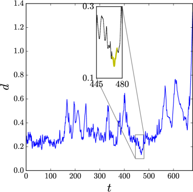
(a)  (b)

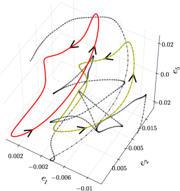
Figure 9: (Colour online) (a) Minimum distance (35) between a long turbulent trajectory ${\hat{a}}_{turb}(t^{\prime})$ and the relative periodic orbit $\textrm{RPO}_{F/6.668}$. Inset: A time interval containing the closest approach. (b) $\textrm{RPO}_{F/6.668}$ (red) and a shadowing segment (corresponding to the inset of panel a) of a turbulent trajectory (dotted line) visualized as a projection onto (33). The closest approach of the turbulent trajectory to $\textrm{RPO}_{F/6.668}$, $d<0.15$, is highlighted yellow.

The above Poincaré sections illustrate the ways in which a relative periodic orbit shapes the geometry of its immediate neighborhood. However, as in the example at hand the unstable manifold Poincaré section is three-dimensional, it is hard to discern any structure in the ergodic sea in two-dimensional projections such as figure 5: in all our Poincaré sections the ergodic sea appears to be structureless cloud, exhibiting no foliation typical of –let’s say– Lorenz attractor or Kuramoto–Sivashinsky attractor (Budanur, 2015). The influence of a relative periodic orbit is here easier to visualize by studying shadowing episodes, i.e., the turbulent trajectory’s visits to a given relative periodic orbit’s neighbourhood, such as figure 9 (a). Here we have defined the minimum distance between trajectories labelled ‘$turb$’ and ‘RPO’ in the fully symmetry-reduced state space (continuous symmetry reduced by (18), the discrete half-rotation symmetry $g_{\theta}$ (5) reduced to the fundamental domain), measured in the energy norm (22), as

$$d(t)=\min_{t^{\prime}\in[0,{T_{\textrm{RPO}}}]}\frac{\left\|\tilde{a}_{turb}(t)-\tilde{a}_{\textrm{RPO}}(t^{\prime})\right\|_{L^{2}}}{\left\|\tilde{a}_{turb}(t)\right\|_{L^{2}}}\,.$$ (35)

Compared to the typical $\textrm{RPO}_{F/6.668}$ linearized neighborhood scales (see figure 6), the yellow shadow in figure 9 (b) is a considerable distance away, but it still completes one co-rotating shadowing period very nicely. Such shadowing episodes offer further support to our main thesis, that relative periodic orbits, together with their stable/unstable manifolds, shape the state-space dynamics within their local neighborhoods.

5.4 Local visualisation: energy norm vs. low pass norm

As our final example of a local visualization of the state space, we examine the local unstable manifold of a travelling wave. The primary goal here is to show with this example is how profoundly the choice of the inner product (or norm) can affect the visualisation, and the conclusions drawn from it. Since in the slice the travelling waves reduce to equilibria, there is no need for a Poincaré section. Therefore, visualizing low-dimensional unstable manifolds of travelling waves is more straightforward compared to those of relative periodic orbits discussed above.

Figure 10 shows a two-dimensional unstable submanifold of $\textrm{TW}_{1.968}$. Note that the unstable manifold of this travelling wave is nine-dimensional ($d_{U}=9$ in table 1). The visualized two-dimensional submanifold corresponds to its most unstable subspace characterized by the largest linear stability exponent of the travelling wave. This dominant exponent is complex valued, with a complex eigen-direction $V_{1}$ which defines a two-dimensional subspace $({\rm Re\,}V_{1},{\rm Im\,}V_{1})$. The three-dimensional visualizations of figure 10 are obtained by projecting each state to the subspace formed by $({\rm Re\,}V_{1},{\rm Im\,}V_{1},V_{2})$ where $V_{2}$ is the third eigen-direction, with a real linear stability exponent.

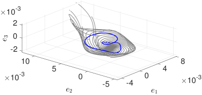
(a) (b)

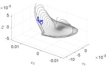
Figure 10: (Colour online) Low-dimensional state space visualisation of the travelling wave $\textrm{TW}_{1.968}$ (origin) and the relative periodic orbit $\textrm{RPO}_{11.696}$ (blue). A two-dimensional unstable submanifold of the travelling wave is approximated by perturbations (gray curves) around the travelling wave (see the text for the details). Both panels show the same objects projected to the same three-dimensional subspace. Two types of inner products are used for the projections: (a) Low pass inner product (23), (b) $L^{2}$ inner product (21).

All computations are carried out in a slice with the travelling wave $\textrm{TW}_{1.968}$ used as the template for symmetry reduction, and placed at the origin of the plots. The unstable submanifold (gray curves) is approximated by forward-integrating several small perturbations to the travelling wave in the direction ${\rm Re\,}V_{1}$. Because of the instability of the travelling wave, the trajectories spiral away from the origin. The spiraling nature of the trajectories is due to the complex stability exponent. In a small neighborhood of the travelling wave, the ensemble of the trajectories approximates the two-dimensional unstable submanifold that is tangent to the plane $({\rm Re\,}V_{1},{\rm Im\,}V_{1})$. Away from the travelling wave this approximation fails and the trajectories diverge.

Also shown in figure 10 is the relative periodic orbit $\textrm{RPO}_{11.696}$ (blue curve). The two panels show the same objects projected to the same subspace $({\rm Re\,}V_{1},{\rm Im\,}V_{1},V_{2})$. The difference is that in panel (a) the low pass inner product (23) is used for the projection while in panel (b) the $L^{2}$ inner product (21) is used.

In the low pass -projection, the relative periodic orbit sits near the travelling wave and appears to be shaped by its unstable manifold. In the $L^{2}$ projection, however, the relative periodic orbit appears to lie rather far from the travelling wave, and there is no hint that their shapes are related. We attribute this to the fact that the low pass norm filters small scale features, assessing the distance between fluid states based on their large-scale structures. In the $L^{2}$ norm, on the other hand, even minute small-scale differences between two states contribute to the computed distance.

We close by noting that the low pass norm was also used to detect near-recurrences of ergodic trajectories. These near-recurrences then served as the initial Newton iteration guesses for obtaining the relative periodic orbits reported in table 1. We find that the recurrences measured in the low pass norm tend to converge to relative periodic orbits more frequently than the recurrences measured in the energy norm. A similar observation was reported by Willis et al. (2013).

6 Conclusion and perspectives

We investigated relative periodic orbits embedded in transitionally turbulent pipe flow confined to a small computational domain. These orbits were found by Newton-type searches, using near-recurrences of the turbulent flow as initial guesses to generate dynamically-relevant solutions. Even in our minimal domain, made small by unphysical symmetry restrictions, this turned out to be a daunting task, practicable only after reduction of problem’s continuous symmetry and, in some cases, requiring also the multiple shooting Newton method.

Nonetheless, we were able to identify 48 distinct relative periodic orbits with numerical precision of $10^{-6}$ or smaller. While this, to the best of our knowledge, is the largest number of periodic orbits for a three-dimensional turbulent flow found so far, the analysis of § 5.2 shows that only some of the state-space visited by turbulence are populated by the set of relative periodic orbits found so far. Nevertheless, our relative periodic orbits do occupy a region of the state space frequently visited by turbulent trajectories, suggesting that additional searches for relative periodic orbits are needed to adequately represent a larger portion of state space. This is consistent with our expectation that in the state space, turbulence is “guided” by the exact invariant solutions.

Our main result is that there is an intrinsic geometry of turbulence, but that one has to explore the Navier–Stokes symmetry-reduced state space very closely in order to discern it. This geometry does not follow from naïve traditional statistical assumptions, as illustrated here by the state-space visualisations of § 5. Principal component analysis (PCA), which we used for global projections of the dynamics in § 5.2, treats turbulent data as if it were a multivariate Gaussian distribution. The true global attractor is in no sense a Gaussian; the intrinsic geometry of turbulence revealed here is dictated by exact time-invariant solutions of Navier–Stokes equations.

Our conclusions are not surprising to a nonlinear dynamicist experienced in working with low-dimensional dynamical systems and their strange attractors, yet the notion that there is an intrinsic geometry to Navier–Stokes long-time dynamics is not as well appreciated in the turbulence community. This under-appreciation is historical, stemming from times when we lacked computational tools to determine the non-trivial exact invariant solutions of Navier–Stokes equations. In this regard, the primary contribution of this paper is the demonstration of the computational feasibility of studying pipe-flow turbulence as a dynamical system. For example, consider figure 5 where 147 individual turbulent runs were necessary to obtain a very rough feeling for how turbulent trajectories are distributed in the state-space. In the dynamical systems approach, it took $8$ carefully chosen trajectories to reveal the shape of $\textrm{RPO}_{F/6.668}$’s unstable manifold.

Given the exploratory nature of this project, many of its intermediate steps were carried out manually, yet most of these could be automated. The first step would be to initiate relative periodic orbit Newton searches by detecting near-recurrences of turbulent flows without human supervision. A slightly more involved step — time-adaptive integration of symmetry-reduced dynamics — will probably be necessary when the azimuthal rotation symmetry is reduced simultaneously with axial translations. We circumvented this issue here by restricting dynamics to the shift-and-reflect invariant subspace, which precludes continuous rotations. This restriction is unphysical and not present in the full problem.

Our explorations of the state-space geometry relied on visualisations of relative periodic orbits and their unstable manifolds. It is already apparent from our data in table 1 that this strategy has limited applicability since all but two invariant solutions we found have unstable manifolds of dimension larger than 3. Even though partial visualisations of the unstable manifold in § 5.3 were insightful, there is no guarantee that this approach can extend to larger computational domains. Ultimately, one needs to develop new methods for systematic study of high-dimensional manifolds, a dynamical notion of ‘distance’ that does not depend on the particular choice of norm, and geometric criteria for distinguishing qualitatively different dynamics in state-space.

In conclusion, we reported here our progress in dynamical study of moderate-Re turbulence in the context of pipe flow. In particular, we demonstrated that embedded within this flow are relative periodic orbits and that they shape dynamics in their respective neighbourhoods through their unstable manifolds. This required various technical obstacles to be overcome, which forced us to restrict this exploratory study to a small symmetry-restricted computational cell. In this sense, we can say that the dynamical approach to turbulence is still in its infancy, but the stage is now set for study of dynamics of wall-bounded shear flow turbulence in its full glory.

Appendix A Multi-point shooting

We used a multi-point shooting method (outlined in this Appendix) in order to find some of the (relative) periodic orbits reported in § 4 (marked with subscript ‘M’ in table 1). For simplicity, we explain the concept for periodic orbits. The approach is essentially the same for relative periodic orbits, once the drifts in the continuous symmetry group directions are accounted for.

Consider a state $a_{0}$ on a periodic orbit with period $T$, i.e.,

$$a_{0}={f^{T}(a_{0})}\,.$$

The periodic orbits are found by searching for the period $T>0$ and the state $a_{0}$ as the zeros of the nonlinear system of equations $a_{0}-{f^{T}(a_{0})}=0$. We determine these zeros from a starting guess by Newton–GMRES–hook iterations (Viswanath, 2007).

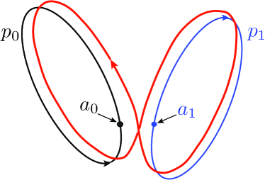
Figure 11: (Colour online) An illustration of the multi-point shooting method. A long periodic orbit (red) is obtained from shorter periodic orbits $p_{0}$ (black) and $p_{1}$ (blue) with periods ${T_{0}}$ and ${T_{1}}$, respectively. Multi-point shooting attempts to find the shortest orbit that shadows both $p_{0}$ and $p_{1}$, with period ${T}$ that is approximately the sum of the periods of the shorter orbits, ${T}\simeq{T_{0}}+{T_{1}}$.

By the semi-group property of the flow map ${f^{t}}$, we have $a_{0}={f^{T}(a_{0})}={f^{t_{2}}({f^{t_{1}}(a_{0})})}\,,$ for any $t_{1},t_{2}>0$ such that $t_{1}+t_{2}=T$. Denoting the time-$t_{1}$ image of $a_{0}$ by $a_{1}={f^{t_{1}}(a_{0})}$, the period closes in two steps

$$a_{1}={f^{t_{1}}(a_{0})}\,,\qquad a_{0}={f^{t_{2}}(a_{1})}\,.$$

The periodic orbit is then found through two-point shooting by searching for states $a_{0}$ and $a_{1}$ as well as the times $t_{1}$ and $t_{2}$ that satisfy

$$a_{1}-{f^{t_{1}}(a_{0})}=0\,,\qquad a_{0}-{f^{t_{2}}(a_{1})}=0\,.$$

The motivation for using the multi-point shooting is two-fold:

1. Let $a_{0}$ be a point on a periodic orbit with period $T$. In theory, we have ${f^{T}(a_{0})}-a_{0}=0$. In practice, $a_{0}$ is never known exactly and only a numerical approximation of it is available. If the periodic orbit is highly unstable, the initial discrepancy grows over time to such extent that the state ${f^{T}(a_{0})}$ might land far away from $a_{0}$. By partitioning the orbit into shorter segments, the error growth is kept under control.

2. Multi-point shooting offers a systematic way to create long orbits by “glueing” the already known shorter orbits (Auerbach et al., 1987). Let $p_{0}$ and $p_{1}$ denote two short periodic orbits with periods $T_{0}$ and $T_{1}$, respectively (see figure 11). The initial guesses for $a_{0}$ and $a_{1}$ are chosen to belong to the shorter orbits, i.e., $a_{0}\in p_{0}$ and $a_{1}\in p_{1}$. The initial guesses for the flight times $t_{1}$ and $t_{2}$ are chosen to coincide with the period of the short orbits, i.e., $t_{1}=T_{0}$ and $t_{2}=T_{1}$. If the Newton–GMRES–hook steps converge, the resulting orbit shadows the short periodic orbits and has a period $T\simeq T_{0}+T_{1}$.

References

- Aubry et al. (1988) Aubry, N., Holmes, P., Lumley, J. L. & Stone, E. 1988 The dynamics of coherent structures in the wall region of a turbulent boundary layer. J. Fluid Mech. 192, 115.
- Auerbach et al. (1987) Auerbach, D., Cvitanović, P., Eckmann, J.-P., Gunaratne, G. & Procaccia, I. 1987 Exploring chaotic motion through periodic orbits. Phys. Rev. Lett. 58, 23.
- Avila et al. (2011) Avila, K., Moxey, D., de Lozar, A., Avila, M., Barkley, D. & Hof, B. 2011 The onset of turbulence in pipe flow. Science 333, 192–196.
- Avila et al. (2013) Avila, M., Mellibovsky, F., Roland, N. & Hof, B. 2013 Streamwise-localized solutions at the onset of turbulence in pipe flow. Phys. Rev. Lett. 110, 224502.
- Avila et al. (2010) Avila, M., Willis, A. P. & Hof, B. 2010 On the transient nature of localized pipe flow turbulence. J. Fluid Mech. 646, 127–136.
- Benedicks & Carleson (1991) Benedicks, M. & Carleson, L. 1991 The dynamics of the Hénon map. Ann. Math. 133, 73.
- Berkooz et al. (1993) Berkooz, G., Holmes, P. & Lumley, J. L. 1993 The proper orthogonal decomposition in the analysis of turbulent flows. Ann. Rev. Fluid Mech. 25, 539–575.
- Budanur (2015) Budanur, N. B. 2015 Exact coherent structures in spatiotemporal chaos: From qualitative description to quantitative predictions. PhD thesis, School of Physics, Georgia Inst. of Technology, Atlanta.