Graph-theoretical evaluation of the inelastic propensity rules for molecules with destructive quantum interference

Abstract

We present a method based on graph theory for evaluation of the inelastic propensity rules for molecules exhibiting complete destructive quantum interference in their elastic transmission. The method uses an extended adjacency matrix corresponding to the structural graph of the molecule for calculating the Green function between the sites with attached electrodes and consequently states the corresponding conditions the electron-vibration coupling matrix must meet for the observation of an inelastic signal between the terminals. The method can be fully automated and we provide a functional website running a code using Wolfram Mathematica, which returns a graphical depiction of destructive quantum interference configurations together with the associated inelastic propensity rules for a wide class of molecules.

I Introduction

Transport through molecules exhibiting quantum interference features due to multiple electronic paths connecting the two leads has been in the past decade a subject of intensive research both theoreticallySolomon et al. (2008); Brisker et al. (2008); Yoshizawa, Tada, and Staykov (2008); Hansen et al. (2009); Markussen, Stadler, and Thygesen (2010, 2011); Solomon et al. (2011); Härtle et al. (2011); Lovey and Romero (2012); Lambert (2015); Pedersen et al. (2014); Geng et al. (2015); Pedersen et al. (2015); Zhao, Geskin, and Stadler (2016); Mitchell et al. (2016); Sam-ang and Reuter (2017) and experimentally.Guedon et al. (2012); Vazquez et al. (2012); Ballmann et al. (2012); Manrique et al. (2015); Bessis et al. (2016) From the very beginning this subject has been addressed not only by direct numerical approaches based on various levels of ab-initio calculations but also by model studies, whose primary task is to bring conceptual understanding of quantum interference effects.Lambert (2015) The idea behind these attempts relies on the believed existence of a connection between basic structural information on a molecule and, at least qualitative, predictive power of some simple analytical procedure (“rule”) indicating the (non)existence and potentially even magnitude of quantum interference effects for the given molecule in a given transport setup.

During the years there appeared a number of such rules formulated either in terms of molecular-orbitalsSolomon et al. (2008); Yoshizawa, Tada, and Staykov (2008); Lovey and Romero (2012); Pedersen et al. (2014) or local tight-binding basis.Markussen, Stadler, and Thygesen (2010, 2011); Stuyver et al. (2015); Geng et al. (2015) The implicit requirement of robustness and simplicity of such rules basically forces them to rely on some very rudimentary properties of the molecular structure, which are often of topological nature and can be described and handled by graph theory. Indeed, such graph-theoretical methods do actually have strong tradition in chemistry in various contexts and flavors. Balaban (1976); Bonchev and Rouvray (1991); Trinajstic (1992) They have been eventually applied also to the problem of quantum interference in electronic transport through molecules. So far, however, their application has been limited to the elastic transmission issue.

In this work, we formulate a graph-theoretical approach to the propensity rules for inelastic electron tunneling spectroscopy (IETS) signals for molecules which exhibit the destructive quantum interference (DQI) in their elastic transmission, i.e., complete elastic current suppression. Interestingly, we find out that the problem can be formulated equivalently to the elastic case with a modified molecular Hamiltonian that includes the electron-vibration coupling matrix. Therefore, all the previous knowledge concerning the elastic case can be straightforwardly transferred to the inelastic problem. Furthermore, to spare readers the necessity of error-prone implementation of elastic graphical rules we present a website which runs efficient and reliable Mathematica code evaluating both the elastic transmission and inelastic IETS propensity rules, using the Wolfram chemical database of molecules.

II Elastic transmission nodes from graph theory

The simplest quantum interference feature studied are the nodes in the elastic transmission caused by the complete destructive quantum interference. In this case, one is only after qualitative information whether or not such a node will be present in the transmission function close to the Fermi energy and, thus, achievable by applying a moderate voltage bias. All the developed different approaches (graphical rules,Markussen, Stadler, and Thygesen (2010) magic ratios,Geng et al. (2015) or the curly arrowStuyver et al. (2015)) rely on the very same underlying approximation of the molecular Hamiltonian by its Hückel form with one local orbital per atom and hopping connectivity determined by the structural graph of the molecule. They subsequently deal differently with this model Hamiltonian, however, they all use the molecular structural graph’s adjacency matrix as the basic Hückel Hamiltonian. This is the core of the graph-theoretical approach that we also adopt here.

It should be mentioned that this starting point is not free of questions. In particular, it is obvious that the Hückel model is largely oversimplified and unrealistic and, therefore, one must ask to what extent can the conclusions drawn from it be taken seriously. A rather thorough comparison of graphical-rules predictions and corresponding DFT calculations for a number of nontrivial molecular structures in Ref. Markussen, Stadler, and Thygesen (2010) showed quite surprising one-to-one correspondence between the two methods. The alleged breakdown of the graphical rules for azulene in Ref. Xia et al. (2014) turned out to be caused by their incorrect application (and was directly contradicted by the experimental data within the same paper Xia et al. (2014)) and, despite its weaknesses discussed in the past year in the literature Stadler (2015); Strange et al. (2015) and also in our Appendix B, the graphical approach seems to provide predictions on the presence/absence of the transmission node with unrivaled accuracy.

Its stunning success can be partly understood by the molecular-orbital point of view Lovey and Romero (2012); Pedersen et al. (2014) — under reasonable assumptions the existence of a transmission node within the HOMO-LUMO gap is determined exclusively by the signs of the HOMO and LUMO molecular-orbital wavefunctions at the sites connected to the leads. Such properties appear to be largely topological, i.e., independent of particular approximations and this explains the perfect agreement between ab-initio DFT approach and simplistic Hückel method. At the same time the exact energetic position of the transmission node (which is always at zero energy for the Hückel model) depends strongly on the used approximation, yet its existence within the HOMO-LUMO gap is a topological property independent of the used method. More elaborate many-body schemes such as GW may reorder the molecular orbitals with respect to DFT and then the predictions on the (non)existence of the transmission node within the HOMO-LUMO gap may differ.Pedersen et al. (2014) Nevertheless, this situation is relevant mostly for molecules weakly coupled to the leads where correlation effects due to local Coulomb interaction on the nearly isolated molecule are significant, which is not the generically studied situation.

The correct formulation of the graphical rules requires for larger molecules an elaborate enumeration and summation of graph diagramsChen (1997), which is prone to error as the case of azulene clearly demonstrated.Xia et al. (2014) For this reason we adopted a safer computer-aided attitude to the problem and developed a Mathematica code interfaced on a webpage http://qi.karlov.mff.cuni.cz:1345 which identifies the elastic DQI molecular configurations as well as calculates the corresponding inelastic propensity rules for them. A print-screen of the webpage is shown in Fig. 1 for the case of the benzene molecule. The user manual from the webpage (red HELP button on the left top) is for convenience of the reader reproduced in Appendix C while technical details about the service are given in Appendix D.

The code evaluates the elastic transmission using the well-known formula (Cuevas and Scheer, 2010, Ch. 8)

$$T_{\mathrm{el}}(\varepsilon)=\mathrm{Tr}\left[\Gamma_{L}G(\varepsilon)\Gamma_{R}G^{\dagger}(\varepsilon)\right],$$ (1)

with

$$G(\varepsilon)\equiv\left(\varepsilon-H_{\mathrm{mol}}+i\frac{\Gamma_{L}+\Gamma_{R}}{2}\right)^{-1},$$

which under the assumption of sufficiently slow energy dependence yields a constant differential conductance $dI/dV=2e^{2}/h\times T_{\mathrm{el}}(\varepsilon_{F})$. Adopting the same approach as Markussen, Stadler, and ThygesenMarkussen, Stadler, and Thygesen (2010) (MST10), i.e. using the Hückel model with one $p_{z}$ orbital per atom and assuming that the leads couple to just single sites (atoms) denoted $L/R$ (left/right) we have

$$\Gamma_{L}=\gamma_{L}|L\rangle\langle L|,\quad\Gamma_{R}=\gamma_{R}|R\rangle\langle R|,$$ (2)

which then implies

$$T_{\mathrm{el}}(\varepsilon_{F})=\gamma_{L}\gamma_{R}|\langle L|G(\varepsilon_{F})|R\rangle|^{2},$$ (3)

and search for the transmission nodes reduces to the evaluation of a specific element of the Green function at the Fermi energy which is set to zero in the Hückel model, i.e. $\varepsilon_{F}\equiv 0$. As explained in Ref. Markussen, Stadler, and Thygesen (2010), if the molecular Hamiltonian $H_{\mathrm{mol}}$ is regular, i.e. $\det(H_{\mathrm{mol}})\neq 0$, the $LR$ matrix element of the full Green function (with the leads included) is zero if and only if the corresponding element of the molecular resolvent $G_{LR}^{0}\equiv\langle L|(\varepsilon_{F}-H_{\mathrm{mol}})^{-1}|R\rangle$ is also zero. Consequently, the existence or not of the DQI between given pairs of atoms is determined exclusively by the molecular structure itself and (within the employed approximations) does not depend on the leads.

After we send a query by means of entering a molecule name, the server responds with the molecule structural formula drawn on top of the page together with its editable graph representation below, see Fig. 1. Now, user must define the subgraph corresponding to the conjugated backbone of the molecule (for details of this crucial operation consult the instructions in the User manual in Appendix C; sometimes the default processing of the molecule by the code without user’s intervention might be sufficient) and then can ask for the calculation of the DQI pattern by pressing the Calculate QI pink button. The code takes the adjacency matrix of the selected subgraph, which (up to a nonzero multiplicative factor) corresponds to the Hückel model Hamiltonian and calculates its inverse (recall that $\varepsilon_{F}\equiv 0$ in this model). Zero entries in this inverse, if they correspond to a pair of vertices (atoms) which can be in principle contacted by leads (typically atoms with hydrogens), are collected and depicted in the graph by orange dashed lines (Fig. 1). These are the configurations which exhibit full DQI in the elastic regime, i.e. for sufficiently small applied voltage below the excitation threshold of molecular vibration modes. For these configurations the code also calculates the inelastic contributions to the conductance (i.e. inelastic propensity rules) as explained in Sec. III which are displayed at the bottom of the webpage under the text Vibration effects on paths with DQI:

There are molecules whose graph representations yield singular matrices, i.e. their determinant is zero and there exist one or more eigenstates exactly at zero energy. Examples of such a situation involve conjugated linear chains with odd number of atoms (propene, pentadiene, etc.) having a single zero mode and cyclobutadiene (corresponding to the square graph, see Appendix B for more details on this very interesting case) with two zero modes. In such cases the above construction equating the full Green function and the molecular resolvent does not hold and one has to use a more careful approach involving the pseudoinverse of the molecular Hamiltonian described in Appendix A. Using this method our code still does find the elastic DQI configurations, but it does not calculate the inelastic propensity rules since the extension of the inelastic theory to this case has not been done yet.

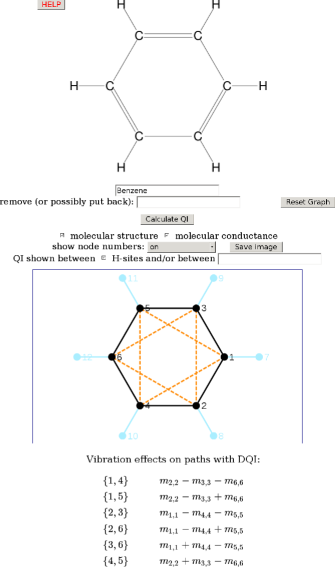
Figure 1: QI webpage with benzene as an example. For description see Sec. II and especially App. C.

III Inelastic propensity rules

III.1 Derivation

Now, we extend the graph-theoretical method to the evaluation of inelastic signals. It was shown more than a decade ago Paulsson, Frederiksen, and Brandbyge (2005); Viljas et al. (2005); de la Vega et al. (2006) that for weak electron-vibration coupling assumed here the inelastic contribution of vibrational mode $\lambda$ to the differential conductance takes on a generic form (Lowest Order Expansion, LOE - see Eqs. (5)–(7) of Ref. Paulsson, Frederiksen, and Brandbyge (2005)) with two (symmetric and asymmetric) universal functions of bias, mode frequency, and temperature multiplied by system-dependent coefficients

$$\Delta_{\lambda}^{\mathrm{Sym}}=\mathrm{Tr}\Big{[}G^{\dagger}\Gamma_{L}G\big{\{}M_{\lambda}G\Gamma_{R}G^{\dagger}M_{\lambda}+\\ +\frac{i}{2}(\Gamma_{R}G^{\dagger}M_{\lambda}AM_{\lambda}-\mathrm{h.c.})\big{\}}\Big{]}.\\ \Delta_{\lambda}^{\mathrm{Asym}}=\mathrm{Tr}\Big{[}G^{\dagger}\Gamma_{L}G\big{\{}\Gamma_{R}G^{\dagger}M_{\lambda}G(\Gamma_{R}-\Gamma_{L})G^{\dagger}M_{\lambda}+\mathrm{h.c.\}}\Big{]},$$ (4)

with the spectral function $A\equiv i(G-G^{\dagger})$ and electron-vibration coupling matrix $M_{\lambda}$. All the Green functions are evaluated at the Fermi energy $\varepsilon_{F}=0$ which corresponds to the wide-band-limit (WBL) assumption of energy-independent $\Gamma$s and $G$ used in the derivation of the above formulas Paulsson, Frederiksen, and Brandbyge (2005). We will justify the validity of this assumption even in cases with DQI shortly, but first let us simplify the above formulas for our Hückel model with leads attached in a configuration exhibiting the elastic DQI, i.e. $\langle L|G(\varepsilon_{F})|R\rangle=0$. Using this property together with Eq. (2) in (4) we find easily that both terms in $\Delta_{\lambda}^{\mathrm{Asym}}$ as well as the two last terms (multiplied by $i/2$) in $\Delta_{\lambda}^{\mathrm{Sym}}$ are zero and we are only left with the first term

$$\Delta_{\lambda}^{\mathrm{Sym}}=\gamma_{L}\gamma_{R}\left|\langle L|GM_{\lambda}G|R\rangle\right|^{2}\approx\gamma_{L}\gamma_{R}\left|\langle L|G_{M_{\lambda}}|R\rangle\right|^{2},$$ (5)

where the second approximate equality holds in the lowest (second) order in $M_{\lambda}$ and we have introduced a modified Green function $G_{M_{\lambda}}$ that is obtained by substituting the molecular Hamiltonian by its modification $H_{\mathrm{mol}}\rightarrow H_{\mathrm{mol}}+M_{\lambda}$. By this step we have reformulated the inelastic problem equivalently to the elastic problem, just with a modified molecular Hamiltonian, see Eqs. (3) and (1) above. The modification involves the electron-vibration coupling matrix $M_{\lambda}$ specific for a given vibrational mode $\lambda$. To keep the Hückel-model approach consistent, we only allow matrix elements of $M_{\lambda}$ to be nonzero on the structural graph of the molecule (more precisely, of the molecular conjugated backbone), i.e. just the diagonals and off-diagonals corresponding to the nearest neighbors connected by a chemical bond.

In principle, we can now adopt some form of the “graphical rules” for the evaluation of the elastic transmission mentioned in Sec. II to the calculation of the matrix element $\langle L|G_{M_{\lambda}}|R\rangle$ of the modified Green function. For this purpose, we use the very same Mathematica-based code which now returns the matrix elements of the modified Green function for all combinations of vertices exhibiting DQI in the elastic transmission. We collect just the linear combinations of the coupling matrix elements neglecting possible $\gamma$-dependent but $M$-independent prefactor and display them in the MathML format at the bottom of the webpage, cf. Fig. 1. According to Eq. (5) their absolute value squared is proportional to the intensity of the inelastic signal for the given vibronic mode, which reveals itself as a jump in the differential conductance at the vibrational excitation threshold $eV_{\mathrm{th}}=\hbar\omega_{\lambda}$. Consequently, they constitute inelastic propensity rules (in the spirit of Eq. (4) in Ref. Paulsson et al. (2008)) which can be used for assessing the effects of molecular symmetries (and/or other factors) for given vibrational modes. Contributions from different vibrational modes are within LOE additive.

III.2 Justification and range of validity

Now, let us discuss the applicability of Eqs. (4) to the case with DQI in elastic transmission. As already mentioned the microscopic derivation of these equations from the non-equilibrium Green functions theory in Refs. Paulsson, Frederiksen, and Brandbyge (2005); Viljas et al. (2005); de la Vega et al. (2006) uses the WBL assumption of energy-independent $G(\varepsilon)$ in the range of order $\hbar\omega_{\lambda}$ around the Fermi energy $\varepsilon_{F}$. The validity of this assumption is certainly not obvious in the DQI case because the Green function $G(\varepsilon)$ passes through zero at the energy of the antiresonance feature (in the Hückel model at the Fermi energy $\varepsilon_{F}=0$) and is finite around it. Thus it is certainly not constant in the relevant energy range. However, it turns out that the width of the elastic antiresonance is usually bigger than the typical vibronic energy and, consequently, $G$ can be reasonably approximated by zero in the whole range.

We illustrate this concept in Fig. 2 where the magnitude of the Green function $|\langle L|G(\varepsilon)|R\rangle|$ for the benzene molecule contacted in the meta position ($L=1,\,R=5$) exhibiting the DQI is plotted both on the linear (upper panel with wider energy scale) as well as logarithmic (lower panel with zoom on low-energy region) scale. The calculation uses the Hückel model with the nearest-neighbor hopping amplitude $2.6$ eV (Cuevas and Scheer, 2010, Sec. 9.5.1, p. 250) and several values of $\gamma\equiv\gamma_{L}=\gamma_{R}$. While on a larger energy scale above $1$ eV the Green function depends strongly on the value of $\gamma$ (top panel), close to zero $|\varepsilon|\lesssim 0.5$ eV the curves collapse (bottom panel) and if we choose our threshold for “machine zero” as $0.01$ eV^-1 (gray dashed horizontal line in the bottom panel corresponding to about 1% of the maximal values of the Green function for not too large $\gamma$s) we see that the “zero value” of the Green function spans the range of roughly $\pm 300$ meV which matches the highest vibrational frequencies of the conjugated backbone corresponding to stretching double and/or triple C-C bonds.

Thus, this rough estimate shows that the usage of Eqs. (4) is justified. Moreover, there exists an extension of Eqs. (4) relaxing the WBL assumption Lü et al. (2014) — comparison of the two approaches by ab-initio treatment Hellmuth, Novotný, and Pauly (2016) of the meta-benzene and 3-methylene-1,4-pentadiyne molecules exhibiting DQI (considered in Refs. Lykkebo et al. (2013, 2014)) yields nearly identical results which further justifies the usage of the WBL formula (4).

Concerning the range of validity of our approach, reader must be aware of the basic fact that the methods works correctly for the Hückel model with equal hoppings between adjacent atoms (if connected by the conjugated backbone). In reality, this assumption may not be realistic and different values of hopping elements might be appropriate at certain links due to, e.g. non-planarity of the molecule (such as biphenyl in Sec. IV.2) or Jahn-Teller distortion (as in cyclobutadiene studied in App. B). In such cases one must be careful and explicitly address the effects of such a modification of the molecular Hamiltonian on the DQI pattern. The results of our code then serve only as the zeroth iteration of a more elaborate study which may survive the refinement of the theory (as in the case of biphenyl where the DQI pattern does not depend on the value of the hopping element in the interlink between the benzene rings) or not (see the Fano resonance analysis in cyclobutadiene at the end of App. B). Unfortunately, there is no a priori general prescription how to decide whether our method is sufficient or not beyond its Hückel model paradigm and one has to assess this case-by-case.

Finally, as the Hückel model only deals with the $\pi$-system and neglects the $\sigma$-system, it is obvious that some of the vibrational modes (those coupled within the $\sigma$-system or coupling $\sigma$-system to the $\pi$-system) are invisible to our approach. This is a shortcoming of our approach and price to pay for the simplification of considering only the $\pi$-system. The results for modes coupling within the $\pi$-system should be, however, fully reliable and relevant. Thus, we may say that our theory gives results only for a (important) subset of vibrational modes, those coupled within the $\pi$-system, which includes various C-C stretching modes etc.

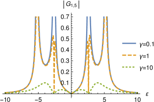
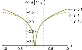
Figure 2: Green function of the meta-benzene for several values of the coupling to the leads $\gamma$ (linear scale in the top panel and low-energy zoom on the logarithmic scale in the bottom panel). We used Hückel hopping element of 2.6 eV according to Ref. (Cuevas and Scheer, 2010, Sec. 9.5.1, p. 250). Values of $\varepsilon$ and $\gamma$ are in eV, of $G$ in eV^-1.

III.3 Physical interpretation

We demonstrate the physical content of our procedure on a simplest example of 3-methylene-1,4-pentadiyne molecule plotted in Fig. 3. Unfortunately, this molecule is not known to the Wolfram chemical database and, thus, our current form of the code cannot directly process it. Nevertheless, we have used manual input into the Mathematica code running at the background of the QI-webpage to obtain the results. Moreover, as can be straightforwardly shown, here the results do not depend on the magnitude of the hopping element at the link $1-6$. As shown in Fig. 3 the end-to-end conductance is suppressed due to DQI which is a consequence of a (broad) Fano resonance analogous to the situation studied in App. B, see Fig. 7. The inelastic propensity rule for this DQI configuration reads $m_{6,6}$, i.e. the IETS signal is nonzero if and only if the onsite electron-vibration matrix element on the apex atom $6$ is non-zero. This can be easily understood in terms of the which-path interferometer. The $4-5$ configuration DQI in the (elastic) transmission is caused by destructive interference of two paths — one is the direct one along the $4-2-1-3-5$ line while the other one is the indirect path $4-2-1-6-1-3-5$ digressing to the side branch. At zero energy these two paths have the same amplitudes and opposite phases and, therefore, cancel out exactly (full elastic DQI).

Now, for sufficient applied voltage bias allowing excitation of a vibrational mode the two paths may become distinguishable, which results in lifting the DQI. This can happen if and only if a vibration is excited at the apex atom $6$ — such a situation allows for an identification of the used (indirect) path and DQI is thus destroyed. On the other hand, vibrations with zero coupling element at the apex atom $m_{6,6}=0$ in principle cannot distinguish the two paths and, consequently, keep the DQI. Therefore, the inelastic propensity rule is proportional solely to the element $m_{6,6}$. We see that the physical principle behind the propensity rule in this case is the simple which-path detection. For molecules with cycles discussed in Sec. IV, the results for the inelastic propensity rules are considerably more complicated, yet, we do believe that the basic physical mechanism behind them is analogous to the present case. From the symmetry of the molecule, it is obvious that all vibrational modes $\lambda^{a}$ antisymmetric with respect to the $1-6$ symmetry axis of the molecule will necessarily have $m_{6,6}^{\lambda^{a}}=0$. Therefore, the simple derived inelastic propensity rule reveals that only symmetric vibrational modes can contribute to the IETS signal of 3-methylene-1,4-pentadiyne.

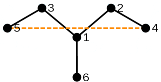
Figure 3: Graph representation of the 3-methylene-1,4-pentadiyne molecule. Only 4–5 DQI is shown, although it occurs also in other configurations.

IV Results for selected molecules

In this section we apply the above-developed formalism to three molecules, namely to benzene, biphenyl, and finally azulene. It should be stated that our choice was somewhat random, selecting from some simple “typical” molecules encountered previously in the literature. Our code can easily handle molecules of much higher complexity and we strongly encourage the readers to experiment with molecule of their choice. Despite the simplicity of our chosen molecules we still make interesting observations concerning their inelastic propensity rules.

IV.1 Benzene

The case of benzene is shown in Fig. 1 in the form of the output on our QI webpage resulting from the “Benzene” query. We can see that the suppressed conductance configurations are just those of the meta position of the leads. This has been well known before. What is less obvious and known is the corresponding inelastic propensity rule which nontrivially combines the diagonal electron-vibration coupling elements on the adjacent sites to the leads. Closer inspection of the rule reveals that the vibronic modes antisymmetric with respect to the axis perpendicular to the connecting line of the leads (e.g., antisymmetric with respect to the $2-5$ axis for the $1-4$ lead configuration) will nullify the expression by the symmetry. Correspondingly, our theory predicts that only the symmetric modes may contribute to the IETS signal. A more detailed quantitative study of this issue will be presented elsewhere. Hellmuth, Novotný, and Pauly (2016)

IV.2 Biphenyl

Results for the biphenyl molecule are shown in Fig. 4, where it is obvious that DQI pattern is rather complex for this more complicated molecule (compared to the previous case of benzene). In particular, the symmetry of the molecule may by overlapping lines obscure which atoms are connected by the DQI lines and which are not. To this end, the possibility of moving the graph vertices on the QI webpage comes very handy and we show the resulting picture with the vertices 1 and 9 moved away from their “equilibrium” positions to reveal the full structure of the DQI network. On the IETS side summarized in Eq. (6), we get specific combinations of (only) diagonal elements of the electron-vibration coupling matrix. What we find interesting is the existence of two nonequivalent DQI configurations ($7-8$ and $7-10$) for which there will be no inelastic signal for all vibronic modes.

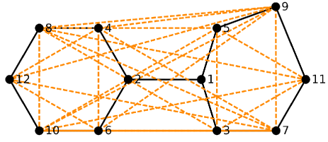
Figure 4: Biphenyl; orange dashed lines connect configurations of leads (substitution patterns) exhibiting elastic DQI. Vertices 1 and 9 are shifted to reveal the otherwise overlapping DQI paths.

$$\begin{array}[]{ll}\left\{3,5\right\}&4m_{1,1}+m_{4,4}+m_{6,6}-4m_{7,7}-4m_{9,9}+m_{12,12}\\ \left\{3,8\right\}&2\left(-m_{4,4}+m_{6,6}+m_{12,12}\right)\\ \left\{3,10\right\}&2\left(m_{4,4}-m_{6,6}+m_{12,12}\right)\\ \left\{3,11\right\}&4m_{1,1}+m_{4,4}+m_{6,6}-4m_{7,7}+4m_{9,9}+m_{12,12}\\ \left\{7,8\right\}&0\\ \left\{7,9\right\}&4\left(m_{3,3}+m_{5,5}-m_{11,11}\right)\\ \left\{7,10\right\}&0\\ \left\{7,12\right\}&2\left(m_{3,3}-m_{5,5}-m_{11,11}\right)\end{array}$$ (6)

IV.3 Azulene

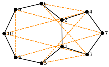
Figure 5: Azulene; orange dashed lines connect configurations of leads (substitution patterns) exhibiting elastic DQI..

Study of an example of non-alternant hydrocarbon, azulene, was motivated by the controversial work Xia et al. (2014) and the results are given in Fig. 5 and Eq. (7). We clearly see that the disputed configuration $3-4$ correctly shows no DQI while the other considered configuration $8-9$ does. We see interesting features in the IETS propensity rules (7) which, contrary to the two previous cases of alternant hydrocarbons, contain the off-diagonal elements of electron-vibration coupling matrix. We conjecture that this property is specific of non-alternant hydrocarbons, which might be worth further research efforts.

$$\begin{array}[]{ll}\left\{3,5\right\}&m_{1,1}+m_{1,2}-m_{1,5}-m_{2,1}-m_{2,2}+m_{2,6}+m_{3,1}-m_{3,7}-m_{4,2}+m_{4,7}-m_{7,7}+m_{8,5}-m_{8,8}-m_{8,10}-m_{9,6}-m_{9,9}+m_{9,10}\\ \left\{3,6\right\}&m_{1,1}+m_{1,2}-m_{1,5}-m_{2,1}-m_{2,2}+m_{2,6}+m_{3,1}-m_{3,7}-m_{4,2}+m_{4,7}-m_{7,7}+m_{8,5}+m_{8,8}-m_{8,10}-m_{9,6}+m_{9,9}+m_{9,10}\\ \left\{3,10\right\}&m_{1,1}+m_{1,2}-m_{1,5}-m_{2,1}-m_{2,2}+m_{2,6}+m_{3,1}-m_{3,7}-m_{4,2}+m_{4,7}-m_{7,7}+m_{8,5}+m_{8,8}-m_{8,10}-m_{9,6}-m_{9,9}+m_{9,10}\\ \left\{7,8\right\}&m_{3,3}-m_{4,4}+m_{5,5}-m_{6,6}-m_{10,10}\\ \left\{8,9\right\}&m_{3,3}+m_{4,4}+m_{5,5}+m_{6,6}-m_{10,10}\end{array}$$ (7)

V Conclusions

We have studied the influence of destructive quantum interference effects in the elastic molecular transmission on the IETS signal via a graph-theoretical approach. We have reformulated the inelastic propensity rules in terms of the elastic problem with a modified molecular Hamiltonian, which allows the application of graph-theoretical methods developed for the elastic case also to the inelastic one. Moreover, we present a Mathematica-based code for the calculation of the destructive quantum interference configurations and inelastic propensity rules, which can be accessed at the webpage http://qi.karlov.mff.cuni.cz:1345. We have demonstrated our method on three simple example molecules of benzene, biphenyl, and azulene, finding a rather complex structure of DQI configurations and interesting features in the inelastic propensity rules.

Our method is designed for a wide community of researchers who are encouraged to play with the developed script and explore its results for new molecules. As an open issue we leave the question of the universality of graph-theoretical results for the inelastic quantities — in particular, whether its prediction are as robust as for the existence of the elastic transmission nodes. Preliminary ab-initio DFT results for the IETS in meta-benzene Hellmuth, Novotný, and Pauly (2016) confirm our prediction for the absence of the asymmetric vibrational modes stemming from the symmetry analysis of the propensity rule, but more checks are certainly needed to validate the method. Another interesting and relevant aspect of the inelastic problem lies in the question whether there is a simple method for assessing the electron-vibration coupling matrix elements not requiring ab-initio calculations as an input. It would be very helpful to have some version of “inelastic Hückel model” which would allow fully analytical study of the inelastic propensity rules. As of today, we are not aware of any such model for the coupling matrix and, in fact, even various ab-initio packages appear to give vastly different results, as we discuss in our upcoming work Hellmuth, Novotný, and Pauly (2016). Thus this issue calls for attention of the IETS research community.

Appendix A Pseudoinverse

If we want to include molecules whose $H_{{\rm mol}}$ has a zero determinant (i.e., $H_{{\rm mol}}$ has a zero eigenvalue), we may proceed in several ways. As shown on the square graphs in Fig. 6 in App. B, one must be careful then. One could, for each leads configuration, add non-zero selfenergies (due to leads as well as infinitesimal $i\eta$s) at relevant places and then calculate the inverse—however, this would be computationally unnecessarily time-consuming. Below we present an alternative way, which is used in our code.

Let $P$ be the projector on the null space of the isolated-molecule Hamiltonian $H_{{\rm mol}}$, i.e., $H_{{\rm mol}}P=PH_{{\rm mol}}=0$, and let $Q=1-P$. Then $PQ=QP=0$. The Green function of an isolated molecule can then be rewritten as

$$\begin{split}G_{0}&=\frac{1}{\varepsilon-H_{{\rm mol}}}=\frac{1}{\varepsilon(P+Q)-QH_{{\rm mol}}Q}=\\ &=\frac{1}{P\varepsilon P+Q(\varepsilon-H_{{\rm mol}})Q}=\frac{P}{\varepsilon}+Q\frac{1}{\varepsilon-H_{{\rm mol}}}Q,\end{split}$$ (8)

valid whenever $(\varepsilon-H_{{\rm mol}})^{-1}$ exists. One infers that in the interesting $\varepsilon\approx 0$ region $G_{0}$ behaves as

$$\begin{split}G_{0}&=\frac{P}{\varepsilon}+\sideset{}{{}^{\prime}}{\sum}_{i}\frac{|i\rangle\langle i|}{\varepsilon-\varepsilon_{i}}=\frac{P}{\varepsilon}-\sideset{}{{}^{\prime}}{\sum}_{i}\frac{|i\rangle\langle i|}{\varepsilon_{i}}\big{(}1+\mathcal{O}(\frac{\varepsilon}{\varepsilon_{i}})\big{)}=\\ &=\frac{P}{\varepsilon}-R(H_{{\rm mol}})+A\varepsilon+\mathcal{O}(\varepsilon^{2}),\end{split}$$ (9)

where in the $i$-summation over eigenvectors of $H_{{\rm mol}}$ we omit the terms corresponding to the zero eigenvalue, $R$ denotes the Moore–Penrose pseudoinverse, and $A$ is $\varepsilon$-independent. Note that $P$ and $R$ are generally hermitian matrices. In our case they are even real symmetric, since here-considered $H_{{\rm mol}}$ is real and symmetric; however, our formulae below do not rely on this special property.

When leads are attached, the system’s Green function is given by $G^{-1}=G_{0}^{-1}-\Sigma$. Due to the assumed localization of $\Sigma$, the $LL$, $LR$, $RL$, $RR$ elements of (retarded) $G$ are simply related in a $2\times 2$ formalism thus

$$\left(\begin{array}[]{cc}G_{LL}&G_{LR}\\ G_{RL}&G_{RR}\end{array}\right)^{-1}=\left(\begin{array}[]{cc}G_{LL}^{0}&G_{LR}^{0}\\ G_{RL}^{0}&G_{RR}^{0}\end{array}\right)^{-1}+\frac{i\gamma}{2}\left(\begin{array}[]{cc}1&0\\ 0&1\end{array}\right).$$ (10)

To calculate conductance we need $G_{LR}$, which can be expressed explicitly as

$$G_{LR}=4\varepsilon\big{(}P_{LR}-\varepsilon R_{LR}+\mathcal{O}(\varepsilon^{2})\big{)}\Big{/}\Big{[}\gamma^{2}(P_{LR}P_{RL}-P_{LL}P_{RR})+{}\\ +\varepsilon\Big{(}2i\gamma(P_{LL}+P_{RR})+\gamma^{2}\big{(}P_{LL}R_{RR}-P_{LR}R_{RL}-P_{RL}R_{LR}+P_{RR}R_{LL}\big{)}\Big{)}+{}\\ +\varepsilon^{2}\Big{(}4-2i\gamma(R_{LL}+R_{RR})-\gamma^{2}\big{(}R_{LL}R_{RR}-R_{LR}R_{RL}+A_{LL}P_{RR}-A_{LR}P_{RL}-A_{RL}P_{LR}+A_{RR}P_{LL}\big{)}\Big{)}+\mathcal{O}(\varepsilon^{3})\Big{]}.$$ (11)

We see that $G_{LR}$ may stay finite around $\varepsilon\approx 0$ only if $P_{LR}P_{RL}-P_{LL}P_{RR}=0$. This is always so if $H_{{\rm mol}}$ does not have a zero eigenvalue ($P=0$), or even when such an eigenvalue exists but is nondegenerate (labelling the corresponding normalized vector $|0\rangle$ gives $P=|0\rangle\langle 0|,$ from which the result immediately follows). For a degenerate zero eigenvalue the combination may or may not be zero. Nonetheless, from the Cauchy–Schwarz inequality $|\langle R|P|L\rangle|^{2}=|\langle R|PP|L\rangle|^{2}\leq\langle L|P|L\rangle\,\langle R|P|R\rangle$ it follows that whenever $P_{LL}$ or $P_{RR}$ is zero, so is $P_{LR}$ (and $P_{RL}$).

If $H_{{\rm mol}}$ does not have a zero eigenvalue ($P=0$), the formula (11) in the $\varepsilon\rightarrow 0$ limit simplifies to

$$G_{LR}^{{}^{\prime}}=\frac{-4R_{LR}}{4-2i\gamma(R_{LL}+R_{RR})-\gamma^{2}(R_{LL}R_{RR}-|R_{LR}|^{2})}.$$ (12)

We could remove $\mathcal{O}$s since the retained denominator cannot become zero: both $R_{LL}$ and $R_{RR}$ would have to be zero to nullify the imaginary part, but then we would be left with $4+\gamma^{2}|R_{LR}|^{2}>0.$ Hence $G_{LR}=0$ just when $R_{LR}=0$, as expected.

If a non-degenerate zero eigenvalue exists, then either (i) both $P_{LL}$ and $P_{RR}$ are zero, then $P_{LR}=P_{RL}=0$, and we once again arrive at Eq. (12), or (ii) at least one of $P_{LL}$, $P_{RR}$ is nonzero (thus positive), the $\varepsilon$-term in the denominator of (11) is necessarily nonzero due to the (single) purely imaginary contribution, and we may disregard the higher-order terms to obtain in the $\varepsilon\rightarrow 0$ limit

$$G_{LR}^{{}^{\prime\prime}}=4P_{LR}\Big{/}\Big{[}2i\gamma(P_{LL}+P_{RR})+{}\\ +\gamma^{2}\big{(}P_{LL}R_{RR}-2\Re(P_{LR}R_{RL})+P_{RR}R_{LL}\big{)}\Big{]}.$$ (13)

Finally, if $H_{{\rm mol}}$ has a degenerate zero eigenvalue, either $|P_{LR}|^{2}-P_{LL}P_{RR}\neq 0$, in which case $G_{LR}=0$, or else the situation is identical to the previous case of nondegenerate zero, Eq. (13).

In any case, we see that from (11) we may—with no assumptions—always remove the $\mathcal{O}(\varepsilon^{2})$ term from the numerator, the $\mathcal{O}(\varepsilon^{3})$ term from the denominator, as well as all the terms containing $A$. In the $\varepsilon\rightarrow 0$ limit we may therefore simplify (11) to

$$G_{LR}=\lim_{\varepsilon\rightarrow 0}4\varepsilon\big{(}P_{LR}-\varepsilon R_{LR}\big{)}\Big{/}\Big{[}\gamma^{2}(|P_{LR}|^{2}-P_{LL}P_{RR})+{}\\ +\varepsilon\Big{(}2i\gamma(P_{LL}+P_{RR})+\gamma^{2}\big{(}P_{LL}R_{RR}-2\Re(P_{LR}R_{RL})+P_{RR}R_{LL}\big{)}\Big{)}+{}\\ +\varepsilon^{2}\Big{(}4-2i\gamma(R_{LL}+R_{RR})-\gamma^{2}(R_{LL}R_{RR}-|R_{LR}|^{2})\Big{)}\Big{]}.$$ (14)

This is the formula used in our program to calculate $G_{LR}$. We stress once more that $P$ and $R$ are characteristics of the isolated molecule ($H_{{\rm mol}}$) and do not depend on leads positions. Although we calculate them only once, equation (14) provides $G_{LR}$ for any leads attachment.

Appendix B Comments on MST10 rules

We have three points to make about the rules proposed in Ref. Markussen, Stadler, and Thygesen (2010), henceforth called the MST10 rules. We only discuss the underlying graph theory and leave aside any practical (im)possibility to chemically realize our graphs.

Sufficiency of $\boldsymbol{\det_{LR}(H_{\mathrm{mol}})=0}$

According to Ref. Markussen, Stadler, and Thygesen (2010), the condition for destructive quantum interference (at $\varepsilon=0$) between molecular sites $L$ and $R$ is given by their Eq. (4), $\det_{LR}(H_{\mathrm{mol}})=0$. However, the latter equation only follows from their equation Eq. (3) (which is our Eq. (15) below with the $i\eta$ terms removed) if the denominator of their Eq. (3) does not vanish. If it does vanish, one ought to be more careful. An example of where this happens is graph A in our Fig. 6.

MST10 derive transmission through a molecule from their Eq. (2), $T(\varepsilon)=\gamma^{2}\left|G_{LR}(\varepsilon)\right|^{2}$ (the same $\gamma$ is used for both leads). Although not stated there, $G_{LR}$ to be considered is either the retarded or the advanced limit (whichever) of the Green function. Hence, if we opt for the latter, MST10’s Eq. (3) should read (for $\varepsilon=0$) in detail

$$G_{LR}=\lim_{\eta\rightarrow 0^{+}}\frac{(-1)^{L+R}\det_{LR}(H_{\mathrm{mol}}+i\eta)}{\det(H_{\mathrm{mol}}+\Sigma_{L}+\Sigma_{R}+i\eta)},$$ (15)

where $\Sigma_{L}$ and $\Sigma_{R}$ are finite advanced self-energies on sites $L$ and $R$, respectively, due to the attached leads; $\det_{LR}(A)$ is the determinant of $A$ from which the $L^{\mathrm{st}}$ row and $R^{\mathrm{th}}$ column were removed. During the $\eta$-limiting process both the numerator and the denominator may approach zero, yet their ratio can stay finite.

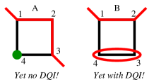
Figure 6: Two graphs for which application of MST10 rules gives wrong prediction.

For the graphs in Fig. 6 $H_{\mathrm{mol}}=\left(\begin{smallmatrix}0&1&0&1\\ 1&0&1&0\\ 0&1&0&1\\ 1&0&1&0\end{smallmatrix}\right)$ (we set our energy unit accordingly). For simplicity we take both nonzero elements of $\Sigma_{L}$ and $\Sigma_{R}$ equal to $\sigma$. In the case of graph A then

$$G_{13}^{\mathrm{A}}=\lim_{\eta\rightarrow 0^{+}}\frac{2i\eta}{4\eta^{2}+\eta^{4}-4i\eta\sigma-2i\eta^{3}\sigma+i\gamma^{2}\eta^{2}}=-\frac{1}{2\sigma}$$ (16)

and stays finite. Especially, if we set $\sigma=i\gamma/2$, $\gamma\in\mathbb{R}$, then $G_{13}^{\mathrm{A}}=i/\gamma$ and we arrive at a unit transmission, $T=1$. We conclude that no destructive interference appears, contrary to the MST10 prediction. Moreover, the result sounds natural, as we have two exactly equivalent paths through the molecule and thus no reason for any destructive interference.

The MST10 rule is correct in specifying when $\det_{LR}(H_{\mathrm{mol}})$ is zero; even in the case above. However, such a zero is not always sufficient to imply zero conductance. Interestingly, the possibility of having $\det(H_{\mathrm{mol}})$ zero is mentioned in Ref. Stadler et al. (2004) (after their Eq. (4)), but it was not elaborated on in any way there. Also, Ref. Pedersen et al. (2015) touches the point in its supplement after their Eq. (3), but only vaguely, and referring to the strength of coupling to the leads, which actually does not play any role in our given example, since it cancels out in the resulting transmission.

Implication vs. equivalence in the MST10 rules

Although the impossibility to draw lines according to the MST10 rules implies that $\det_{LR}(H_{\mathrm{mol}})$ is zero (simply because this impossibility means that all the terms in the determinant expansion are zero), one should not—contrary to what the other MST10 rule says—expect that a possibility to draw one MST10-rules-complying diagram automatically leads to a nonzero $\det_{LR}(H_{\mathrm{mol}})$. This is exemplified by graph B in Fig. 6. Here

$$G_{12}^{\mathrm{B}}=\lim_{\eta\rightarrow 0^{+}}\frac{\eta^{2}}{4\eta^{2}+\eta^{4}-4i\eta\sigma-2i\eta^{3}\sigma-\sigma^{2}-\eta^{2}\sigma^{2}}=0,$$

the denominator does not vanish and only the numerator, i.e., $\det_{LR}(H_{\mathrm{mol}})$ plays a significant role. Thus we could actually avoid the use of $\eta$, just as the original MST10 procedure would do. Anyway, we obtain zero, while the MST10 rules predict it nonzero.

The problem is that the ability to draw a graph complying to the MST10 rules only means that there is a corresponding nonzero term in the $\det_{LR}(H_{\mathrm{mol}})$ expansion, not that the sum of all such terms with possibly varying signs is nonzero. Drawing a conclusion from just one graph like B in Fig. 6 is erroneous, all contributing graphs must be taken into account.

In this respect, it should be clearly stated that the relevant MST10 rule reading “If such a continuous path can be drawn, then the condition (4) is not fulfilled and a transmission antiresonance does not occur at the Fermi energy.” is incorrect. By omitting this fact, the comment Stadler (2015) on the rules’-breakdown article Xia et al. (2014) only prolonged the misunderstanding of some, which shows itself in the reaction to the comment, Strange et al. (2015) stumbling on this very point. Hopefully though, the necessity to consider all the graphs seems now to have been (re-)established Markussen, Stadler, and Thygesen (2011); Pedersen et al. (2015); we note that the old paper Stadler et al. (2004) actually did use the summation.

Fano resonance in the square

Above in this appendix we discussed conductance of a square with leads attached to the opposite corners, Fig. 6A, and we saw the conductance (at zero energy and for a symmetric leads attachment) is equal to unity (see below Eq. (16)). While this is true, there is an interesting extra point worth mentioning: if one tries and calculates conductance of a distorted square in which not all the hopping elements are the same, one finds that even an infinitesimal distortion leads to an abrupt decrease of the conductance from one to zero, a fact that perhaps deserves a comment.

First, the fact that we need $i\eta$ (and not just a finite $i\gamma$) to ascertain that the inverse of $H_{\mathrm{mol}}$ exists suggests that there is a completely decoupled, i.e., for transport irrelevant, molecular eigenstate at zero energy. This is confirmed explicitly after changing the basis from states $\left\{\left|1\right\rangle,\left|2\right\rangle,\left|3\right\rangle,\left|4\right\rangle\right\}$ (localized at the individual sites) to $\left\{\left|1\right\rangle,\left|+\right\rangle,\left|3\right\rangle,\left|-\right\rangle\right\}$ with $\left|+\right\rangle\equiv 1/\sqrt{2}\big{(}|2\rangle+|4\rangle\big{)}$ and $\left|-\right\rangle\equiv 1/\sqrt{2}\big{(}|2\rangle-|4\rangle\big{)}$. In this basis $H_{\mathrm{mol}}^{{}^{\prime}}=\sqrt{2}\left(\begin{smallmatrix}0&1&0&0\\ 1&0&1&0\\ 0&1&0&0\\ 0&0&0&0\end{smallmatrix}\right)$. We see that the system is actually equivalent to a 3-site linear chain with all the hoppings equal to $\sqrt{2}$ and zero on-site energies plus a completely isolated state. The chain (as any similar chain with odd number of sites) has unity transmission (at zero energy) when connected to leads at its ends, here sites 1 and 3. This is the result we expect.

Figure 7: Equivalence of an $a111$-disturbed square and a chain with a branch.

Second, if we disturb one hopping from 1 to $a$, say, between sites 1 and 2—we call the disturbance $a111$—, and again do the transformation, see Fig. 7, we obtain $H_{\mathrm{mol}}^{{}^{\prime}a111}=\frac{\sqrt{2}}{2}\left(\begin{smallmatrix}0&a+1&0&a-1\\ a+1&0&2&0\\ 0&2&0&0\\ a-1&0&0&0\end{smallmatrix}\right)\approx\sqrt{2}\left(\begin{smallmatrix}0&1&0&\xi\\ 1&0&1&0\\ 0&1&0&0\\ \xi&0&0&0\end{smallmatrix}\right)$, where $\xi\equiv(a-1)/2\ll 1$. This means that what before was an isolated state now weakly couples to the chain. And this is the archetypal characteristics of systems displaying the Fano resonance, see (Cuevas and Scheer, 2010, Sec. 13.6). The formula (13.17) of the reference describes transport through a single site (i.e., a 1-site chain) coupled to leads as well as to a single other site with potentially different on-site energy. Our current case is similar, though on-site energies are all zero and we have a 3-site chain. Explicit calculation gives in the small-$\varepsilon$ limit and for $\xi/\gamma\ll 1$ transmission

$$T(\varepsilon\approx 0)=\frac{1}{1+\big{(}\frac{2\xi^{2}}{\varepsilon\gamma}\big{)}^{2}}=\frac{1}{1+\big{(}\frac{(a-1)^{2}}{2\varepsilon\gamma}\big{)}^{2}},$$ (17)

which is essentially the reference’s equation (with $\epsilon=\epsilon_{0}=0$, $t=\sqrt{2}\xi$). We see our system displays a coexistence of two processes: (i) in energy smoothly behaving transport along the chain and (ii) a sharp (if $a$ is close to one) Fano resonance positioned at $\varepsilon=0$, i.e., at the very place where the former smooth part would otherwise have a maximum. Fig. 8 depicts this situation.

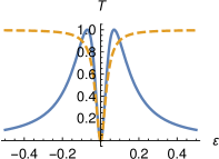
Figure 8: Fano resonance in transmission $T$ through an $a111$-deformed square, see Fig. 7, with $\gamma=0.3$ and $a=1.07$. Blue (full) line is the full $\varepsilon$-dependence while orange (dashed) line is its small-$\varepsilon$ approximation (17).

If both the 1–2 and 3–4 hoppings were changed to $a$ (disturbance $a1a1$), the state $|-\rangle$ would (after the transformation) connect equally well to the $|1\rangle$ and $|3\rangle$ states, with the strength of $\sqrt{2}\xi$, and the transmission would again include the Fano resonance (the denominator in Eq. (17) would be $1+(\frac{2(2\xi)^{2}}{\varepsilon\gamma})^{2}$).

In contrast, changing hoppings 1–2 and 4–1 to $a$ (i.e., in a ‘symmetric’ way; disturbance $a11a$) keeps the $|-\rangle$ state perfectly decoupled, irrespective of $a$, and the transmission remains unity with no Fano feature present—as if the square were perfect.

Appendix C User manual

NB

Check the tooltips shown when you position the mouse over the entry fields. After modifying any field press Enter there to reconsider the value; pink color indicates changed but not yet considered values.

Molecule entry

Enter the molecule name and press Enter to fetch the molecular data. Molecules that are ‘autocompleted’ are arenes known to Wolfram Alpha (as of 7/2016); however, any molecule known to Wolfram Alpha can actually be entered. You can also use molecule’s CAS, CID, and perhaps also other shown numbers. (E.g., entering Azulene, CID9231, and CAS275-51-4 yields the same.) The request can take some time, usually about 15 seconds.

Preparation for conductance calculation

Before calculating conductance it is the user’s responsibility to prepare the relevant graph skeleton that should be composed only of the molecule’s conjugated (π-bonded) subsystem(s). (Hence, one generally removes at least the hydrogen atoms.)

Atoms listed in the ‘remove (or possibly put back):’ entry are (if existent) removed or reclaimed upon pressing Enter. Operations are carried out in the written order, a leading ‘+’ indicates reclamation, otherwise removal takes place. Atoms are removed together with all attached edges. Atoms can be designated by their label (‘5’), by their type (‘H’), or by their type augmented by the number of attached edges (‘C:4’). After fetching molecular data, we by default remove H and C:4 from the graph, since this is what one naturally almost always wants. However, one can explicitly bring the atoms and related edges back, using the provided tools, or more straightforwardly by pressing the ‘Reset Graph’ button. Both atoms and edges can be removed and/or reclaimed by right-clicking them. Removal of an atom removes also the attached edges, removal of an edge removes only the edge. Reclamation of an atom reclaims only the atom, reclamation of an edge brings back its end atoms as well. Atoms and edges removed from the molecular graph are shown in light blue. Only objects in black enter conductance calculation. The ‘remove (or possibly put back):’ entry field does not try to reflect all the changes made to the graph (e.g. with mouse clicks). It only serves as a means of input for a single-shot operation.

Conductance and vibration effects calculation

Calculation of conductance is started by clicking the ‘Calculate QI’ button. Dashed orange lines connect sites between which (total) destructive quantum interference (DQI) takes place, effectively zeroing elastic transmission. Note that such lines do not connect atoms not belonging to the same conjugated part of the molecule (then, although we have zero conductance, it is not due to interference, but due to effective electrical isolation). The DQI (i.e., dashed orange) lines are only shown between (i) atoms to which a hydrogen atom is attached in the molecule, if the ‘H-sites’ checkbox is checked, and/or (ii) any atoms whose labels (numbers) have been inputted in the for-this-purpose reserved field. If the considered-graph adjacency matrix has no inverse, the user obtains a warning about zero-energy-mode(s) existence, along with the zero-energy-eigenvalue degeneracy. For this case we still provide the elastic conductance output, however, not the effect of vibrations (the topic has not been fully investigated by us yet). One should also be careful with the interpretation of the results then, especially if several zero-energy modes exist, since molecules in such cases rather undergo distortions (not accounted for here), rendering provided predictions suspect at least. More studies in this direction are needed. The ‘Vibration Effects’ table shows combinations of electron-vibration-interaction (EVI) matrix elements, one for each currently displayed path featuring DQI. An absolute-square of each such combination is the functional dependence of the lowest-order change of the originally zero (due to DQI) conductance on the EVI matrix elements. The ‘Vibration Effects’ table is in the MathML format, allowing reuse. [A right-click on the table offers ‘Show Math As’, ‘MathML Code’; this can be copied to the clipboard (often ctrl-a ctrl-c) and inserted to a MathML-aware application (such as LibreOffice: Insert - Object - Formula, Tools - Import MathML from Clipboard). MathML can also be saved to a file and/or converted to TeX, e.g. by an online tool here.]

Additional information

Graph nodes can be moved with the mouse. The graph can be moved as a whole by dragging and can be resized with the mouse wheel. The graph can be, in its current state, saved by pressing the ‘Save image’ button. Pressing the ‘Reset Graph’ button resets the controls and the graph to the initial state, even before the default removal of H and C:4. The checkboxes ‘molecular structure’ and ‘molecular conductance’ toggle the visibility of molecular-structure and molecular-conductance edges, respectively. The latter case is only applicable after conductance has been calculated. The ‘show node numbers:’ menu controls the visibility of node labels (the numbers next to nodes).

Appendix D Code details

Service overview

Our program is accessible as a web service at http://qi.karlov.mff.cuni.cz:1345. Fig. 1 depicts a screenshot of the web page with calculated conductance for benzene. To use the service, a web browser with enabled javascript is necessary. The details about service usage are provided under the Help button of the page. Fig. 9 shows the service building blocks together with their relations. In order to provide a lucid representation of results, we use an interactive graph-drawing (javascript) library sigma.js sig . Its built-in interactivity allows easy rearrangement of graph layouts, which alleviates the frequent problem of line overlaps. Sigma.js library gets downloaded to the client’s browser from our server upon directing the browser to our service. The server runs the node.js framework nod .

Input parameters for a calculation are taken from the web page and sent via the server as parameters to Mathematica Wolfram Research, Inc. (2016) scripts that do the calculation. The results are, via standard output and error streams, returned to the server, which relays them to the client’s browser for display.

The Mathematica component provides, besides the fairly simple computational part described below, access to the Wolfram Research chemical database, from which chemical structures of molecules are retrieved as graphs. While this may limit the number of available molecules, this information source relieves the burden of data entry.

Figure 9: Program building blocks.

Mathematica scripts

In the following, numbers enclosed in angle brackets denote lines of the commented code.

The first Mathematica script is used to retrieve structural information about the molecule entered on the web page. It reads an argument from the command line to see what molecule is to be processed $\langle 1\rangle$, tries to fetch a graph of the molecule structure from the ChemicalData database $\langle 9\rangle$, and saves it to the variable g. A picture of the graph in the Portable Network Graphics (PNG) format is sent Base64-encoded (since we use text streams) to the output $\langle 19\rangle$. This is the picture one sees on the web page. Note that in the output stream we delimit individual information pieces with tags, such as M-PNG-Base64 $\langle 18,20\rangle$, used on the client’s side to distinguish the information. The rest of the script builds a JavaScript Object Notation (JSON) object populated with all needed information about the molecule $\langle$22–34$\rangle$, and outputs it $\langle$36–44$\rangle$. JSON objects are easily handled by the sigma.js library, which draws the interactive graph in the client’s browser.

⬇

1material = $CommandLine[[-1]];

2Print[”MOLECULE”];

3Print[material];

4Print[”/MOLECULE”];

5

6(*get the data about the material*)

7(*we do two checks since, for some reason, the response from

8 Mathematica can vary*)

9g = Check[ChemicalData[material, ”StructureGraph”],

10 Write[”stderr”, ”Molecule name not known.”]; Quit[]];

11If[MissingQ[g], Write[”stderr”, ”Molecule name not known.”];

12 Quit[]];

13(*seems easier to get VertexTypes from ChemicalData than

14 from the graph g*)

15gVTypes = ChemicalData[material, ”VertexTypes”]

16

17(*output PNG of the molecule graph*)

18Print[”M-PNG-Base64”];

19Export[$Output, ExportString[g, ”PNG”], ”Base64”];

20Print[”/M-PNG-Base64”];

21

22nodes = MapThread[{”id” $\rightarrow$ ToString[#1],

23 ”label” $\rightarrow$ ToString[#1],

24 ”x” $\rightarrow$ #2[[1]], ”y” $\rightarrow$ -#2[[2]],

25 ”type” $\rightarrow$ ToString[#3]} &,

26 {VertexList[g], PropertyValue[g, VertexCoordinates], gVTypes}

27 ];

28

29nEdges = Length[EdgeList[g]];

30edges = MapThread[Flatten[List[#1, #2]] &,

31 {Thread[”id” $\rightarrow$ Map[”e” <> ToString[#] &,

32 Range[nEdges]]],

33 ({”source” $\rightarrow$ ToString[#1], ”target” $\rightarrow$ ToString[#2]} &)

34 @@@ EdgeList[g]}];

35

36Print[”JSON”];

37Check[

38 Export[$Output,

39 {”nodes” $\rightarrow$ nodes,

40 ”edges” $\rightarrow$ edges},

41 ”JSON”], Write[”stderr”, ”Graph export failed.”]; Quit[],

42 Export::badval];

43Print[];

44Print[”/JSON”];

After we determine, by removing vertices and/or edges from the original graph, what the conjugated part of the molecule really is, we send the modified graph to a second Mathematica script, which does the calculation proper. Again, the graph is passed on the command line (as a string) $\langle 47\rangle$. For the graph we determine the adjacency matrix gAM $\langle 56\rangle$, and proceed along the lines of Appendix A, i.e., by calculating the pseudoinverse R $\langle 47\rangle$, projector P $\langle$72–3$\rangle$, and $G_{LR}$ in the $\varepsilon\rightarrow 0$ limit, in the code denoted by GijLim $\langle$75–83$\rangle$, c.f. Eq. (14). Zero $G_{LR}$, if the sites $L$ and $R$ are connected in the considered graph, means there is a total destructive quantum interference (DQI) present, the fact which we note down to QI $\langle$85–94$\rangle$ and output as a list of edges where DQI occurs $\langle$100–2$\rangle$.

Finally, we calculate the effect of vibration modes on the conductance of paths that without vibrations feature complete destructive interference. It is (for the present) only calculated for the case when $H_{\mathrm{mol}}$ has no zero eigenvalue $\langle 106\rangle$. As we discuss in the main text, we introduce an electron-vibration coupling matrix M having nonzero elements on its diagonal and between sites that are directly connected in the graph $\langle$108–9$\rangle$, and evaluate $G_{0}MG_{0}$ $\langle 110\rangle$ (if $H_{\mathrm{mol}}$ has no zero eigenvalue, $G_{0}=-R$), absolute-square of which is proportional to the lowest-order vibration-induced change in the conductance. For each originally zero-conductance path we output the related combination of matrix-$M$ elements (to be absolute-squared). We send such a table in the MathML format to the client $\langle$134–6$\rangle$.

⬇

1(*graph as a string like

2 gStr = ”{{n1,n2},{n2,n3},{n3,n4},{n4,n5},{n5,n6},{n6,n1}}”;*)

3gStr = $CommandLine[[-1]];

4

5edges = UndirectedEdge[#[[1]], #[[2]]] & /@ ToExpression[gStr];

6g = Graph[edges];

7v = VertexList[g];

8

9vLen = Length[v];

10zM = ConstantArray[0, {vLen, vLen}];

11

12gAM = AdjacencyMatrix[g];

13

14R = PseudoInverse[gAM];

15

16(*normed basis of nullspace of gAM*)

17ns = (#/Norm[#] &) /@ NullSpace[gAM];

18nsDeg = Length[ns];

19

20Print[”NS_DEGENERACY”];

21Print[nsDeg];

22Print[”/NS_DEGENERACY”];

23

24(*and corresponding projectors*)

25PPerVector = Outer[Times, #, #] & /@ ns;

26

27(*projector onto the whole nullspace*)

28P = Apply[Plus, PPerVector];

29If[P == 0, P = zM];

30

31G[i_, j_] := (4 P[[i, j]] \[Omega] + 4 R[[i, j]] \[Omega]^2) /

32 ((P[[i, j]]^2 - P[[i, i]] P[[j, j]]) \[Gamma]^2 +

33 \[Gamma] (2 I P[[j, j]] - P[[j, j]] R[[i, i]] \[Gamma] +

34 2 P[[i, j]] R[[i, j]] \[Gamma] + P[[i, i]] (2 I - R[[j, j]] \[Gamma])) \[Omega] +

35 (4 + 2 I R[[j, j]] \[Gamma] + R[[i, j]]^2 \[Gamma]^2 +

36 R[[i, i]] \[Gamma] (2 I - R[[j, j]] \[Gamma])) \[Omega]^2)

37

38Gij = Table[G[i, j], {i, vLen}, {j, vLen}];

39GijLim = Map[Limit[#, \[Omega] $\rightarrow$ 0] &, Gij, {2}];

40

41(*zero elements of GijLim are replaced with 1, nonzero with 0*)

42QI = Map[If[# === 0, 1, 0] &, GijLim, {2}];

43

44(*There is no real QI between disconnected parts*)

45gDistM = GraphDistanceMatrix[g];

46gConnM = Map[If[# == Infinity, 0, 1] &, gDistM, {2}];

47QI = QI gConnM;

48

49(*zero the diagonal*)

50QI = ReplacePart[QI, {i_, i_} $\rightarrow$ 0];

51

52gQI = AdjacencyGraph[v, QI];

53eQI = EdgeList[gQI];

54eQIList = Apply[List, eQI, {1}];

55

56Print[”EQI”];

57Print[eQIList];

58Print[”/EQI”];

59

60(*Phonon part, now only when there is no zero energy

61 in the spectrum*)

62If[nsDeg == 0,

63 (*create a matrix M that lives on g*)

64 M = (Outer @@ {Subscript[m, #1, #2] &, #, #} & @ v)

65 (gAM + IdentityMatrix[Length[v]]);

66 GMG = R.M.R; (*NB we use the pseudoinverse*)

67

68 pWith1 = Position[QI, 1]; (*where is 1 in QI?*)

69 If[Length[pWith1] == 0, phononsEffect = ”No path with DQI present”,

70 p = Pick[pWith1, (#[[1]] < #[[2]]&) /@ pWith1];

71

72 GMGQI = GMG[[#[[1]], #[[2]]]] & /@ p; (*consider paths with QI*)

73

74 (*let’s get rid of fractions*)

75 Ph = GMGQI Det[gAM] // Simplify;

76 (*just a simple check for a leading minus sign; can’t make it

77 worse, can it?*)

78 Ph = If[Characters[ToString[#, InputForm]][[1]] == ”-”, -#, #]& /@ Ph;

79 (*mapping between positions and vertices*)

80 e = v[[#]]& /@ p;

81

82 e = Sort /@ e;

83 ePh = MapThread[List, {e, Ph}];

84 ePh = Sort[ePh, #1[[1]] < #2[[1]] &];

85

86 Mtable = TableForm[ePh, TableDepth $\rightarrow$ 2];

87 phononsEffect = ExportString[Mtable, ”MathML”];

88 ]

89

90 Print[”PHONONQI”];

91 Print[phononsEffect];

92 Print[”/PHONONQI”];

93]

References

- Solomon et al. (2008) G. C. Solomon, D. Q. Andrews, R. H. Goldsmith, T. Hansen, M. R. Wasielewski, R. P. Van Duyne, and M. A. Ratner, Journal of the American Chemical Society 130, 17301 (2008), pMID: 19053483, http://dx.doi.org/10.1021/ja8044053 .
- Brisker et al. (2008) D. Brisker, I. Cherkes, C. Gnodtke, D. Jarukanont, S. Klaiman, W. Koch, S. Weissman, R. Volkovich, M. C. Toroker, and U. Peskin, Molecular Physics 106, 281 (2008), http://dx.doi.org/10.1080/00268970701793904 .
- Yoshizawa, Tada, and Staykov (2008) K. Yoshizawa, T. Tada, and A. Staykov, Journal of the American Chemical Society 130, 9406 (2008), pMID: 18576639, http://dx.doi.org/10.1021/ja800638t .
- Hansen et al. (2009) T. Hansen, G. C. Solomon, D. Q. Andrews, and M. A. Ratner, The Journal of Chemical Physics 131, 194704 (2009).
- Markussen, Stadler, and Thygesen (2010) T. Markussen, R. Stadler, and K. S. Thygesen, Nano Letters 10, 4260 (2010), http://dx.doi.org/10.1021/nl101688a .
- Markussen, Stadler, and Thygesen (2011) T. Markussen, R. Stadler, and K. S. Thygesen, Phys. Chem. Chem. Phys. 13, 14311 (2011).
- Solomon et al. (2011) G. C. Solomon, J. P. Bergfield, C. A. Stafford, and M. A. Ratner, Beilstein Journal of Nanotechnology 2, 862 (2011).
- Härtle et al. (2011) R. Härtle, M. Butzin, O. Rubio-Pons, and M. Thoss, Physical Review Letters 107, 046802 (2011).
- Lovey and Romero (2012) D. A. Lovey and R. H. Romero, Chemical Physics Letters 530, 86 (2012).
- Lambert (2015) C. J. Lambert, Chemical Society Reviews 44, 875 (2015).
- Pedersen et al. (2014) K. G. L. Pedersen, M. Strange, M. Leijnse, P. Hedegård, G. C. Solomon, and J. Paaske, Phys. Rev. B 90, 125413 (2014).
- Geng et al. (2015) Y. Geng, S. Sangtarash, C. Huang, H. Sadeghi, Y. Fu, W. Hong, T. Wandlowski, S. Decurtins, C. J. Lambert, and S.-X. Liu, Journal of the American Chemical Society, Journal of the American Chemical Society 137, 4469 (2015).
- Pedersen et al. (2015) K. G. L. Pedersen, A. Borges, P. Hedegård, G. C. Solomon, and M. Strange, The Journal of Physical Chemistry C 119, 26919 (2015), http://dx.doi.org/10.1021/acs.jpcc.5b10407 .
- Zhao, Geskin, and Stadler (2016) X. Zhao, V. Geskin, and R. Stadler, The Journal of Chemical Physics, The Journal of Chemical Physics 146, 092308 (2016).
- Mitchell et al. (2016) A. K. Mitchell, K. G. L. Pedersen, P. Hedegaard, and J. Paaske, (2016), arXiv:1612.04852 .
- Sam-ang and Reuter (2017) P. Sam-ang and M. G. Reuter, (2017), arXiv:1702.01341 .
- Guedon et al. (2012) C. M. Guedon, H. Valkenier, T. Markussen, K. S. Thygesen, J. C. Hummelen, and S. J. van der Molen, Nat Nano 7, 305 (2012).
- Vazquez et al. (2012) H. Vazquez, R. Skouta, S. Schneebeli, M. Kamenetska, R. Breslow, L. Venkataraman, and M. S. Hybertsen, Nat Nano 7, 663 (2012).
- Ballmann et al. (2012) S. Ballmann, R. Härtle, P. B. Coto, M. Elbing, M. Mayor, M. R. Bryce, M. Thoss, and H. B. Weber, Physical Review Letters 109, 056801 (2012).
- Manrique et al. (2015) D. Z. Manrique, C. Huang, M. Baghernejad, X. Zhao, O. A. Al-Owaedi, H. Sadeghi, V. Kaliginedi, W. Hong, M. Gulcur, T. Wandlowski, M. R. Bryce, and C. J. Lambert, Nature Communications 6, 6389 EP (2015).
- Bessis et al. (2016) C. Bessis, M. L. Della Rocca, C. Barraud, P. Martin, J. C. Lacroix, T. Markussen, and P. Lafarge, Scientific Reports 6, 20899 EP (2016).
- Stuyver et al. (2015) T. Stuyver, S. Fias, F. De Proft, and P. Geerlings, The Journal of Physical Chemistry C, The Journal of Physical Chemistry C 119, 26390 (2015).
- Balaban (1976) A. T. Balaban, ed., Chemical Applications of Graph Theory (Academic Press, London, 1976).
- Bonchev and Rouvray (1991) D. Bonchev and D. Rouvray, eds., Chemical Graph Theory: Intorduction and Fundamentals, Mathematical Chemistry, Vol. 1 (Gordon and Breach Science Publishers, 1991).
- Trinajstic (1992) N. Trinajstic, Chemical Graph Theory, 2nd ed., Mathematical chemistry series (CRC Press, 1992).
- Xia et al. (2014) J. Xia, B. Capozzi, S. Wei, M. Strange, A. Batra, J. R. Moreno, R. J. Amir, E. Amir, G. C. Solomon, L. Venkataraman, and L. M. Campos, Nano Letters 14, 2941 (2014), pMID: 24745894, http://dx.doi.org/10.1021/nl5010702 .
- Stadler (2015) R. Stadler, Nano Letters 15, 7175 (2015), pMID: 26485189, http://dx.doi.org/10.1021/acs.nanolett.5b03468 .
- Strange et al. (2015) M. Strange, G. C. Solomon, L. Venkataraman, and L. M. Campos, Nano Letters 15, 7177 (2015), pMID: 26485067, http://dx.doi.org/10.1021/acs.nanolett.5b04154 .
- Note (1) Very recently, two works Zhao, Geskin, and Stadler (2016); Sam-ang and Reuter (2017) have addressed in detail general questions concerning the DQI origin, predictability and classification.
- Chen (1997) W.-K. Chen, Graph Theory and Its Engineering Applications, Advanced Series in Electrical and Computer Engineering, Vol. 5 (World Scientific, Singapore, 1997).
- Cuevas and Scheer (2010) J. C. Cuevas and E. Scheer, Molecular Electronics: An Introduction to Theory and Experiment, World Scientific Series in Nanoscience and Nanotechnology (World Scientific, New Jersey, 2010) p. 703.
- Paulsson, Frederiksen, and Brandbyge (2005) M. Paulsson, T. Frederiksen, and M. Brandbyge, Phys. Rev. B 72, 201101 (2005).
- Viljas et al. (2005) J. K. Viljas, J. C. Cuevas, F. Pauly, and M. Häfner, Phys. Rev. B 72, 245415 (2005).
- de la Vega et al. (2006) L. de la Vega, A. Martín-Rodero, N. Agraït, and A. L. Yeyati, Phys. Rev. B 73, 075428 (2006).
- Paulsson et al. (2008) M. Paulsson, T. Frederiksen, H. Ueba, N. Lorente, and M. Brandbyge, Phys. Rev. Lett. 100, 226604 (2008).
- Lü et al. (2014) J.-T. Lü, R. B. Christensen, G. Foti, T. Frederiksen, T. Gunst, and M. Brandbyge, Physical Review B 89, 081405 (2014).
- Hellmuth, Novotný, and Pauly (2016) T. Hellmuth, T. Novotný, and F. Pauly, “Destructive quantum interference effects on the inelastic electron tunneling spectroscopy propensity rules,” (2016), in preparation.
- Lykkebo et al. (2013) J. Lykkebo, A. Gagliardi, A. Pecchia, and G. C. Solomon, ACS Nano, ACS Nano 7, 9183 (2013).
- Lykkebo et al. (2014) J. Lykkebo, A. Gagliardi, A. Pecchia, and G. C. Solomon, The Journal of Chemical Physics 141, 124119 (2014).
- Note (2) For example, we ignore the chemical instability of the cyclobutadiene represented by the square graph in Fig. 6, which we use just for illustration of our points.
- Stadler et al. (2004) R. Stadler, S. Ami, C. Joachim, and M. Forshaw, Nanotechnology 15, S115 (2004).
- Note (3) Since Fano resonances often occur to a side from other extrema, they often have an asymmetric-in-energy signature. Not so it happens, however, in our case.
- (43) sigma.js, http://sigmajs.org.
- (44) node.js, https://nodejs.org.
- Wolfram Research, Inc. (2016) Wolfram Research, Inc., Mathematica 11.0 (2016), http://www.wolfram.com.