Importance-sampling computation of statistical properties of coupled oscillators

Abstract

We introduce and implement an importance-sampling Monte Carlo algorithm to study systems of globally-coupled oscillators. Our computational method efficiently obtains estimates of the tails of the distribution of various measures of dynamical trajectories corresponding to states occurring with (exponentially) small probabilities. We demonstrate the general validity of our results by applying the method to two contrasting cases: the driven-dissipative Kuramoto model, a paradigm in the study of spontaneous synchronization; and the conservative Hamiltonian mean-field model, a prototypical system of long-range interactions. We present results for the distribution of the finite-time Lyapunov exponent and a time-averaged order parameter. Among other features, our results show most notably that the distributions exhibit a vanishing standard deviation but a skewness that is increasing in magnitude with the number of oscillators, implying that non-trivial asymmetries and states yielding rare/atypical values of the observables persist even for a large number of oscillators.

I Introduction

Non-linear dynamical systems often exhibit different behavior in different regions of the phase space. A prominent example is the Fermi-Pasta-Ulam chain of non-linear oscillators, for which a variation in the initial condition leads to physically very different long-time solutions, e.g., solitons and chaotic breathers Gallavotti:2007 . Another example is the generic co-occurrence of regular (quasiperiodic) and chaotic trajectories in Hamiltonian systems MacKay:1987 . Even when trajectories leading to one type of behavior are rare or atypical, they may still be responsible for important physical phenomena. An example is that of chemical reactions in which the system goes over from being constituted with one chemical species to another, due to atypical trajectories passing through unstable saddle point regions in the phase space Komatsuzaki:2002 . It is thus of great interest to identify and characterize the variation in dynamical evolution with respect to initial conditions and the occurrence of atypical dynamical trajectories in many-body non-linear systems.

A different motivation to study atypical trajectories and dependence on initial conditions arises from a theorist’s endeavor to reconcile analytical calculations done in the thermodynamic limit, $N\to\infty$, with numerical simulations for a finite number $N$ of particles. Calculations often assume that for generic dynamical systems, different initial conditions have similar behavior, which may be justified on heuristic grounds in the limit $N\to\infty$. A pertinent question for finite $N$ is however to ask to what extent the infinite-$N$ scenario holds and what is the role of initial conditions. Specifically, one may ask for a finite-$N$ system: Do most initial conditions behave similarly to that predicted in theory, so that the latter is indeed the typical behavior for a finite system? Or is there a significant fraction of initial conditions that show large deviations with respect to the theoretically predicted behavior? What is the relative fraction of these two types of behavior (atypical vs. typical), and how does this fraction approach zero (if at all) as $N\rightarrow\infty$? While a resolution of these issues helps to view objectively analytical predictions vis-à-vis numerical simulations, one obtains as an offshoot a quantitative view of the variability of phase space regions.

In this work, we address the aforementioned issues in a system of coupled oscillators, which offers a useful framework to connect low-dimensional systems studied in the field of non-linear dynamics with the high-dimensional ones dealt with in statistical mechanics Strogatz:2014 . In specific limits, the system we consider describes the equilibrium, second-order, conservative dynamics of a paradigmatic long-range interacting system, and a non-equilibrium, first-order, dissipative dynamics in the presence of disorder that describes a prototypical model of spontaneous collective synchronization. Two specific observables that we focus on to bring out the dependence on initial conditions for finite systems are (i) the finite-time Lyapunov exponent (FTLE), and (ii) a time-averaged order parameter, both quantifying the variability in the finite-time dynamical evolution of trajectories starting from different initial conditions.

The computational challenge we tackle in this paper is the efficient estimation of the probability of an observable computed over an ensemble of states, and in particular, the probability of occurrence of atypical values away from the typical value of the observable. Estimation of probability of rare events is a traditional problem in statistical physics (tackled, e.g., using Monte Carlo methods Newman:2002 ). In the last decade, the issue of rare-event simulation has seen a surge in interest in a number of varied contexts involving non-linear dynamical systems Kurchan:2007 . In this work, we accomplish the desired task of computation of probability by starting from the framework of a Metropolis-Hastings Monte Carlo method proposed in Ref. Leitao:2017 for rare-event simulation in simple chaotic maps, and by suitably adapting the method to apply to the more complex dynamics of coupled oscillators. Our method allows us to study systems involving thousands of coupled oscillators, in contrast to small systems ($\sim 32$ degrees of freedom) considered previously Kurchan:2007 ; Leitao:2017 . A successful implementation of our algorithm demonstrates the generality of our method and results with respect to the two different observables, namely, the FTLE and the time-averaged order parameter, and with respect to two very different and contrasting dynamics, namely, an equilibrium, second-order, conservative dynamics, and a non-equilibrium, first-order, dissipative dynamics in presence of disorder. Besides this technical accomplishment, the results obtained with our method reveal that the distribution of both the FTLE and the time-averaged order parameter contains useful information about the dynamics in the stationary state and about how finite-size effects come into play in determining the nature of stationary-state fluctuations. In particular, we show that the distributions are significantly skewed even in the limit $N\to\infty$, thereby implying the existence of very different typical and atypical behavior. Our results therefore underline the crucial role of initial conditions in dictating the dynamical behavior, thereby cautioning against naive reliance on analytically-predicted typical behavior in complex dynamical systems.

The paper is organized as follows. In Sections II and III, we introduce respectively the model and the method of study used in our paper. Numerical findings and a quantification of the efficiency of our method are discussed in Section IV, while conclusions are drawn in Section V. Some of the technical details are presented in the three appendices.

II Model

Our model comprises $N$ globally-coupled oscillators note-rotor . The phase $\theta_{i}\in[0,2\pi)$ and the angular velocity $v_{i}$ of the $i$-th oscillator, $i=1,2,\ldots,N$, evolve in time according to

$$\frac{{\rm d}\theta_{i}}{{\rm d}t}=v_{i},$$

(1)

$$m\frac{{\rm d}v_{i}}{{\rm d}t}=\gamma(\omega_{i}-v_{i})-\frac{K}{N}\sum_{j=1}^{N}\frac{\partial u(\theta_{j}-\theta_{i})}{\partial\theta_{i}},$$

where $m$ is the moment of inertia and $\omega_{i}$ is the natural frequency of the $i$-th oscillator. The $\omega_{i}$’s are quenched disordered random variables obtained from a common distribution $g(\omega)$. Here, the second term on the right hand side of the second equation describes the torque due to an all-to-all coupling between the oscillators, with $u(\theta)$ being the mean-field interaction potential. The coupling constant $K$ in Eq. (1) is scaled down by $N$ to have a well-defined behavior of the associated term in the thermodynamic limit $N\to\infty$, while the parameter $\gamma$ describes the tendency of each individual oscillator to adapt its angular velocity to its natural frequency.

Mean-field interactions, such as in Eq. (1), are a special case (i.e., $\alpha=0$) of long-range interactions that decay asymptotically with the interparticle distance $r$ as $r^{-\alpha}$, with $0\leq\alpha\leq d$ in $d$ spatial dimensions Campa:2009 ; Bouchet:2010 ; Campa:2014 ; Gupta:2017 . Long-range interacting (LRI) systems abound in nature, e.g., self-gravitating systems, non-neutral plasma, dipolar ferroelectrics and ferromagnets, two-dimensional geophysical vortices, wave-particle interacting systems such as free-electron lasers, etc Campa:2014 .

In the dynamics (1), $u(\theta)$ being even in $\theta$ note-torque , on using $u(\theta)=u(\theta+2\pi)$, and taking $u(0)=0$ without loss of generality, a Fourier expansion yields

$$u(\theta)=\sum_{s=1}^{\infty}\widetilde{u}_{s}\Big{[}1-\cos(s\theta)\Big{]}.$$ (2)

Different choices of the set $\{\widetilde{u}_{s}\}$ allow to describe a broad class of oscillator systems. Here, taking $\widetilde{u}_{1}=1,\widetilde{u}_{s>1}=0,K>0$, we consider two interesting and very different limits of the dynamics:

(i) $\gamma\to 0$: Eq. (1) then describes the Hamiltonian mean-field (HMF) model, a paradigmatic model of long-range interactions Ruffo:1995 ; Dauxois:2002 . The dynamics is given by

$$\frac{{\rm d}\theta_{i}}{{\rm d}t}=v_{i},~{}~{}m\frac{{\rm d}v_{i}}{{\rm d}t}=\frac{K}{N}\sum_{j=1}^{N}\sin(\theta_{j}-\theta_{i}),$$ (3)

which conserves the total energy and the total momentum $m\sum_{i=1}^{N}v_{i}$, and admits a Boltzmann-Gibbs equilibrium stationary state.

(ii) $m\to 0$: Eq. (1) then defines the Kuramoto model, a prototypical model of spontaneous synchronization in interacting dynamical systems Kuramoto:1975 ; Kuramoto:1984 ; Strogatz:2000 ; Pikovsky:2001 ; Acebron:2005 ; Strogatz:2003 ; Gupta:2014 :

$$\frac{{\rm d}\theta_{i}}{{\rm d}t}=\omega_{i}+\frac{\widetilde{K}}{N}\sum_{j=1}^{N}\sin(\theta_{j}-\theta_{i});~{}\widetilde{K}=\frac{K}{\gamma}.$$ (4)

Note that the dynamics (4) is first order, is intrinsically dissipative, with the set of $\omega_{i}$’s continuously pumping energy into the system. In the presence of thermal noise, the dynamics relaxes at long times to a non-equilibrium stationary state Gupta:2014 .

The collective dynamics of the oscillators is quantified by the quantities

$$\Big{(}R^{(x)}_{s},R^{(y)}_{s}\Big{)}\equiv\frac{1}{N}\sum_{j=1}^{N}\Big{(}\cos(s\theta_{j}),\sin(s\theta_{j})\Big{)},$$ (5)

in terms of which Eq. (1) reads

$$\frac{{\rm d}\theta_{i}}{{\rm d}t}=v_{i},$$

(6)

$$m\frac{{\rm d}v_{i}}{{\rm d}t}=\gamma(\omega_{i}-v_{i})$$

$$+K\sum_{s=1}^{\infty}s\widetilde{u}_{s}\Big{[}-R^{(x)}_{s}\sin(s\theta_{i})+R^{(y)}_{s}\cos(s\theta_{i})\Big{]},$$

which shows that the dynamics is that of a single oscillator in a self-consistent mean field due to its interaction with other oscillators. Associated with the $s$-th Fourier mode of the interaction potential is the magnitude of the mean field given by $R_{s}=\sqrt{[R^{(x)}_{s}]^{2}+[R^{(y)}_{s}]^{2}}$. Here, $R_{1}$ measures phase coherence among all the oscillators, and its stationary-state average $\langle R_{1}\rangle$ has been invoked as the clustering or the magnetization order parameter in the HMF model Ruffo:1995 , and as the synchronization order parameter in the Kuramoto model Kuramoto:1975 .

In its equilibrium state, the HMF model in the thermodynamic limit $N\to\infty$ exhibits either a clustered (magnetized) ($\langle R_{1}\rangle>0$) phase or a homogeneous (unmagnetized) ($\langle R_{1}\rangle=0$) phase, depending on whether the energy per oscillator $\epsilon$ is below or above a critical value $\epsilon_{c}\equiv 3K/4$, respectively, with a continuous phase transition at $\epsilon_{c}$ Ruffo:1995 . It is convenient to depict the phases of the oscillators as points that are moving on a unit circle under the dynamics (3). Then, in the clustered phase, the points depicting the oscillator phases are clustered together on the unit circle at any instant of time. By contrast, in the homogeneous phase, the points are independently and uniformly distributed on the unit circle. In the thermodynamic limit, the evolution of each oscillator phase becomes equivalent to that of a pendulum in a constant gravitational field, so that no chaos but periodic orbits are expected. For finite $N$, however, the oscillators have the complex nonlinear dynamics (3) that may be characterized by a spectrum of Lyapunov exponents (LE) ${\lambda_{i}}$, with $i=1,\ldots,2N$ Pikovsky:2016 . Numerical simulations and analytical arguments for equilibrium initial conditions have demonstrated that the maximal LE (MLE) vanishes with increasing $N$ in the homogeneous phase. On the other hand, the MLE has a finite value for energies just below $\epsilon_{c}$, while far below $\epsilon_{c}$, the MLE vanishes for large $N$ Latora:1998 ; Firpo:1998 ; Latora:1999 ; Manos:2011 ; Filho:2017 . A recent study has shown that in the clustered phase, the MLE is strictly positive for large $N$, converging to its asymptotic value with $1/\ln N$ corrections Ginelli:2011 .

In contrast to the HMF model, fewer studies of the chaotic properties of the Kuramoto model exist. In the thermodynamic limit, the model shows a stationary-state transition from a low-$\widetilde{K}$ unsynchronized phase $(\langle R_{1}\rangle=0)$ to a high-$\widetilde{K}$ synchronized phase $(\langle R_{1}\rangle>0)$ at the critical coupling $\widetilde{K}_{c}=2/[\pi g(\langle\omega\rangle)]$, where $\langle\omega\rangle\equiv\int{\rm d}\omega~{}\omega g(\omega)$ is the average frequency Kuramoto:1975 ; moreover, $g^{\prime\prime}(\langle\omega\rangle)>0$ (respectively, $g^{\prime\prime}(\langle\omega\rangle)<0$) leads to a first-order (respectively, a continuous) transition. Viewing the Kuramoto dynamics in a co-rotating frame moving uniformly with angular frequency $\langle\omega\rangle$, time snapshots of the oscillator phases on the unit circle in the unsynchronized and the synchronized phase are identical to those in the homogeneous and the clustered phase of the HMF model, respectively. In the thermodynamic limit, the Lyapunov spectrum has been analytically shown to be flat and equal to zero below the transition, while above the transition, both a flat and a negative branch coexist Radons:2005 . Simulations for finite $N$ have shown the existence of a large MLE $\lambda_{1}(N)$ above the transition Popovych:2005 , with $\lambda_{1}(N)\sim N^{-\alpha};~{}\alpha\leq 1$ Popovych:2005 ; Pikovsky:2016 .

In the rest of the paper, we use interchangeably the terms “magnetized” and “synchronized” to describe the clustered phase in both the HMF model and the Kuramoto model, and the terms “unmagnetized” and “homogeneous” to describe the unsynchronized phase in the two models.

Let us note that all the aforementioned studies of both the HMF model and the Kuramoto model have considered the LE’s (and mostly, the MLE) when computed over a fixed time and averaged over a finite set of initial conditions, while it is evidently of interest to analyze the higher moments of the MLE. Here, we are motivated to study the chaotic properties of these systems by going beyond the average behavior of the MLE and examining in close detail the distribution of the finite-time LE (the FTLE) with respect to different initial conditions (distributed with the equilibrium measure in the HMF model, and with the stationary-state measure in the Kuramoto model). Our goal is to obtain the scaling with $N$ of these distributions, with a particular emphasis on the tails (atypical/rare chaotic properties). Additionally, under the same conditions and with the same focus, we obtain the distribution of the time-averaged synchronization order parameter (TASOP). In Appendix A, we define both the quantities of interest, namely, the FTLE and the TASOP. In light of the highly non-linear and many-body nature of both the HMF dynamics and the Kuramoto dynamics, the program of obtaining the desired distributions is plagued with the usual computational challenges associated with simulations of high-dimensional non-linear systems with complex phase spaces. In the next section, we report on our implementation of a dedicated importance sampling algorithm that addresses these challenges, and is particularly suited to sample rare events in many-body interacting systems, such as the ones described by Eq. (1).

III Method

The main challenge in estimating the tails of the distribution of any observable $O_{\cal T}$ (e.g., the FTLE, $O_{\cal T}\equiv\lambda_{\cal T}$, and the TASOP, $O_{\cal T}\equiv R_{\cal T}$, see Appendix A) is the rarity (exponentially small probability of occurrence) of events that contribute to the tails. We address this challenge by employing a Monte-Carlo Metropolis-Hastings algorithm developed in Ref. Leitao:2017 . In essence, this algorithm uses importance sampling to draw states that are more likely to be on the tails of the distribution of the observable, while remaining unbiased on the averages it computes. This algorithm was developed in Ref. Leitao:2017 to exclusively sample continuous phase spaces of chaotic systems. However, its usefulness was tested only in low-dimensional (i.e., $\sim 32$ degrees of freedom) chaotic systems evolving in discrete times. The main result of this work is to report on a suitable adaptation and implementation of the algorithm for higher-dimensional chaotic systems evolving in continuous times, which allows to reliably estimate even for very large $N\sim 2^{10}$ the mean, and, specifically, the higher moments of any observable $O_{\cal T}$.

Let ${\bf r}(t)$ denote a state of the system at time $t$, and $\{{\bf r}(\tau);~{}\tau\in[0,{\cal T}]\}$ the trajectory obtained by evolving ${\bf r}(t)$ for time ${\cal T}$ according to ${\rm d}{\bf r}(t)/{\rm d}t={\bf F}({\bf r}(t))$, so that at the end of the evolution, our observable of interest has the value $O_{\cal T}({\bf r}(t))$. Here, ${\bf r}(t)$ is the $2N$-dimensional vector of phases and angular velocities of the $N$ oscillators: $r_{1,2,\ldots,N}=\theta_{i=1,2,\ldots,N}$ and $r_{N+1,N+2,\ldots,2N}=v_{i=1,2,\ldots,N}$ in the HMF model, and is the $N$-dimensional vector of phases of the $N$ oscillators: $r_{1,2,\ldots,N}=\theta_{i=1,2,\ldots,N}$ in the Kuramoto model. Our objective is to estimate the distribution $\rho(O_{\cal T})$ of $O_{\cal T}$ for a given time ${\cal T}$, a given system size $N$, and a given distribution of the initial conditions ${\bf r}(t)$ over a phase space region of size $\Omega$. A knowledge of $\rho(O_{\cal T})$ obviously allows to obtain any moment of $O_{\cal T}$. We are particularly interested in estimating the moments of $O_{\cal T}$ higher than the mean, which characterize the tails of $\rho(O_{\cal T})$.

The Metropolis-Hastings algorithm draws states ${\bf r}$ according to a sampling distribution $\pi({\bf r})$ that favors states yielding the tails of $\rho(O_{\cal T})$ Newman:2002 . We use the so-called canonical-ensemble version of the algorithm, which has

$$\pi({\bf r})\propto e^{-\beta O_{\cal T}({\bf r})},$$ (7)

where $\beta$ is a parameter, a “fictitious” temperature, that we may tune to favor states with higher $O_{\cal T}$ (lower $\beta<0$) or lower $O_{\cal T}$ (higher $\beta>0$). Note that with $\beta=0$, one has a sampling distribution that is uniform over $\Omega$, so that every initial state is equally likely to be sampled. Hence, as far as computing the distribution of $O_{\cal T}$ is concerned, a uniform sampling will merely favor the most likely values of $O_{\cal T}$, that is, values of $O_{\cal T}$ in and around the peak of $\rho(O_{\cal T})$.

In our implementation of the algorithm, we also employ the choice (7). The outcome of our algorithm is a sequence of states, ${\bf r}\to{\bf r}^{\prime}\to{\bf r}^{\prime\prime}\to\ldots$, that are empirically distributed according to $\pi({\bf r})$, which we use to estimate $\rho(O_{\cal T})$. Generally, the sequence is correlated, and therefore, we evaluate the efficiency of the algorithm by estimating how the integrated autocorrelation increases with $N$. To obtain the states ${\bf r}$, the algorithm employs a traditional Markov chain with a proposal and an acceptance rate of new states. Our implementation is based on the method developed in Ref. Leitao:2017 , with two important modifications we introduce to apply it to systems of oscillators. The first modification is the use of continuous time (the algorithm in Ref. Leitao:2017 was formulated for discrete-time dynamics). The second modification is the way we propose the states. Below, we systematically describe the essential steps of the algorithm (details in Appendix B).

In the following, $U[a,b]$ denotes a random number uniformly distributed in the interval $[a,b]$, and $\mathcal{N}(0,1)$ denotes a Gaussian-distributed random number with mean zero and variance unity. Also, unless stated otherwise, the index $i$ runs over $1,2,\ldots,N_{\rm tot}$, where $N_{\rm tot}$ is the total number of degrees of freedom: $N_{\rm tot}=2N$ for the HMF model, and $N_{\rm tot}=N$ for the Kuramoto model.

III.1 Preparing the initial state ${\bf r}$

The initial state ${\bf r}$ of the sequence ${\bf r}\to{\bf r}^{\prime}\to{\bf r}^{\prime\prime}\to\ldots$ may be prepared according to the purpose of study. For example, for the results discussed in the paper, we sample the state according to the equilibrium distribution in the HMF model and according to the stationary-state distribution in the Kuramoto model. We consider for the HMF model a net zero momentum and an energy density above the critical value $\epsilon_{c}$, so that the system is in an unsynchronized equilibrium state (We choose $K=1$ so that $\epsilon_{c}=3/4$). Correspondingly, the phases are uniformly and independently distributed in $[0,2\pi)$, while the angular velocities are Gaussian distributed; the mean of the Gaussian distribution is zero, while the variance has to be chosen such that the prepared state has the desired energy at which one wants to perform the study. The details of the latter step are given in Appendix B. For the Kuramoto model, we consider a Gaussian distribution with zero mean and unit variance for $g(\omega)$; knowing the corresponding $\widetilde{K}_{c}=2\sqrt{2/\pi}\approx 1.6$, we work with $\widetilde{K}<\widetilde{K}_{c}$, such that the system is in an unsynchronized stationary state; correspondingly, the phases are uniformly and independently distributed in $[0,2\pi)$. Note that the mentioned choices for either the HMF model or the Kuramoto model are for illustrative purposes, and any other choice is equally good. Once prepared, one estimates the observable $O_{\cal T}({\bf r})$ corresponding to the initial state ${\bf r}$.

III.2 Given state ${\bf r}$, proposing a new state ${\bf r}^{\prime}$

Given the state ${\bf r}$, we propose a new state ${\bf r}^{\prime}$ by perturbing ${\bf r}$ as ${\bf r}^{\prime}={\bf r}+\bm{\delta}$, where $\delta_{i}$’s are random variables sampled independently from a half-Gaussian: ${\rm Prob}(\delta_{i})=\sqrt{2}/(A\sqrt{\pi})\exp\Big{(}-\delta_{i}^{2}/(2A^{2})\Big{)}$, with $A\equiv\sigma({\bf r})\sqrt{\pi/2}$. Here, the quantity $\sigma({\bf r})$ is determined from the estimated value of $O_{\cal T}({\bf r})$, as

$$\sigma({\bf r})\equiv\sigma_{0}\exp[-|O_{\cal T}({\bf r})|t^{\star}({\bf r})],$$ (8)

where $\sigma_{0}\sim O(1)$ is a given parameter, and $t^{\star}$ is related to the time needed for $O_{\cal T}({\bf r}^{\prime})$ to diverge from $O_{\cal T}({\bf r})$. Following Ref. Leitao:2017 , we use

$$t^{\star}({\bf r})\equiv{\rm max}\Big{(}0,{\cal T}-\Big{|}\frac{a-1}{\beta\Big{(}O_{\cal T}^{{\rm mp}}-O_{\cal T}({\bf r})\Big{)}}\Big{|}\Big{)},$$ (9)

where $O_{\cal T}^{{\rm mp}}$ is the most probable value of the observable note-O-mp , and $0<a<1$ is a constant related to the desired acceptance rate (e.g., $a=0.01$). In this way of preparing the proposed state, it is ensured that when ${\bf r}$ is on the tail of the distribution $\rho(O_{\cal T})$, the proposed state is more likely to also be on the tail. On the other hand, when ${\bf r}$ is close to the peak of the distribution $\rho(O_{\cal T})$, the proposed state would correspond to a region around either the peak or the tail of $\rho(O_{\cal T})$ Leitao:2017 . In the case of the HMF model, whose dynamics conserves the total energy and the total momentum, one has to implement additional steps to make sure that the proposed state has the same momentum (namely, zero momentum) and the same energy as the initial state. The former is ensured by computing the average velocity $v_{\rm avg}$ of the proposed state, as $v_{\rm avg}=\sum_{i=1}^{N}v_{i}/N$, and then shifting the velocity of each oscillator, as $v_{i}\to v_{i}-v_{\rm avg}$; Energy conservation is ensured by following the steps 2-6 of Appendix B.

III.3 Accepting the proposed state ${\bf r}^{\prime}$

Once prepared, the proposed state ${\bf r}^{\prime}$ is accepted with a probability that ensures that the distribution of $O_{\cal T}$ corresponding to the sequence of states ${\bf r}\to{\bf r}^{\prime}\to{\bf r}^{\prime\prime}\to\ldots$ that is eventually sampled is given by Eq. (7); this is achieved by ensuring that generation and acceptance of proposed states satisfy the condition of detailed balance Newman:2002 :

$$\pi({\bf r})W({\bf r}\to{\bf r}^{\prime}) =\pi({\bf r}^{\prime})W({\bf r}^{\prime}\to{\bf r}),$$ (10)

where we have the transition probability

$$W({\bf r}\to{\bf r}^{\prime}) \equiv g({\bf r}^{\prime}|{\bf r})P_{{\rm accept}}({\bf r}^{\prime}).$$ (11)

Here, $g({\bf r}^{\prime}|{\bf r})$ gives the probability of proposing the state ${\bf r}^{\prime}$, given state ${\bf r}$, while $P_{{\rm accept}}({\bf r}^{\prime})$ is the probability of accepting the state ${\bf r}^{\prime}$. Using Eq. (11) in Eq. (10) gives

$$\frac{P_{{\rm accept}}({\bf r}^{\prime})}{P_{{\rm accept}}({\bf r})}=\frac{\pi({\bf r}^{\prime})g({\bf r}|{\bf r}^{\prime})}{\pi({\bf r})g({\bf r}^{\prime}|{\bf r})}=\exp\Big{[}-\beta\Big{(}O_{\cal T}({\bf r}^{\prime})-O_{\cal T}({\bf r})\Big{)}\Big{]}\frac{\Big{(}1/\sigma({\bf r}^{\prime})\Big{)}\exp\Big{(}-|{\bf r}-{\bf r}^{\prime}|^{2}/[\pi\sigma^{2}({\bf r}^{\prime})]\Big{)}}{\Big{(}1/\sigma({\bf r})\Big{)}\exp\Big{(}-|{\bf r}-{\bf r}^{\prime}|^{2}/[\pi\sigma^{2}({\bf r})]\Big{)}}.$$ (12)

Corresponding to the condition (12), one may compute the ratio $R\equiv\sigma({\bf r})/\sigma({\bf r}^{\prime}),$ and then the quantity

$$r\equiv\log(R)-\frac{|{\bf r}-{\bf r}^{\prime}|^{2}}{\pi\sigma^{2}({\bf r})}\Big{(}R^{2}-1\Big{)}-\beta(O_{\cal T}({\bf r}^{\prime})-O_{\cal T}({\bf r})){\cal T}.$$ (13)

Then, provided a uniformly generated random number $u\sim U[0,1]$ satisfies $\log(u)<r,$ we accept the proposed state: ${\bf r}\to{\bf r}^{\prime}$, record the new value of $O_{\cal T}$ given by $O_{\cal T}({\bf r}^{\prime}),$ and also do the updates: $t^{\star}(O_{\cal T}({\bf r}))\to t^{\star}(O_{\cal T}({\bf r}^{\prime}))$ and $\sigma({\bf r})\to\sigma({\bf r}^{\prime})$. Otherwise, we do not perform any updates, and record the old value of $O_{\cal T}$ given by $O_{\cal T}({\bf r})$.

Repeating the steps detailed in Sections III.2 and III.3, we finally generate a sequence of $M$ states ($M$ of the order of several thousands), and, correspondingly, a sequence of $M$ values of $O_{\cal T}$, which are then used to construct the desired distribution $\rho(O_{\cal T})$ by suitably unbiasing Landau:2014 for the bias introduced by the choice of (7) in the sampling of the states.

IV Results

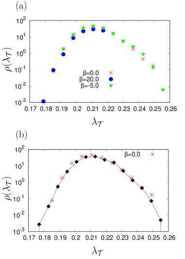
Figure 1: (Color online) Our proposed Monte Carlo method leads to improved estimation of atypical states in coupled oscillators. The distribution of the FTLE $\lambda_{\cal T}$, Eq. (25), was estimated numerically using different values of the bias parameter $\beta$ in the sampling distribution (7). Results for three values of $\beta$, namely, $\beta=-5.0,\beta=0.0,\beta=20.0$, are shown in panel (a), while a combination of the results for these three values of $\beta$ gives the solid black (diamond) curve in panel (b). The system studied is the HMF model (3) with coupling constant $K=1$ and energy density $\epsilon=2.0$, and we used ${\cal T}=10.0$.

Implementing the algorithm developed in Section III, we now present numerical results for the two systems discussed in Section II – the HMF model, Eq. (3), and the Kuramoto model, Eq. (4) – and for the two observables introduced in Section II and Appendix A – the FTLE $\lambda_{\cal T}$ and the TASOP $R_{\cal T}$. Our first objective is to show the suitability of our algorithm in achieving our set-out goals. Figure 1 shows the effect of changing the bias $\beta$ in the sampling distribution (7) on the estimation of $\rho(\lambda_{\cal T})$. On varying $\beta$, as desired, we obtain improved estimations of $\rho(\lambda_{\cal T})$ at different range of values of $\lambda_{\cal T}$ (panel (a)). Combining the results obtained with different $\beta$’s leads to an improved estimate of the tails of $\rho(\lambda_{\cal T})$, when compared to the case of $\beta=0$ (panel (b)). This success prompts us to apply our method to investigate the $N$-dependence of the distribution.

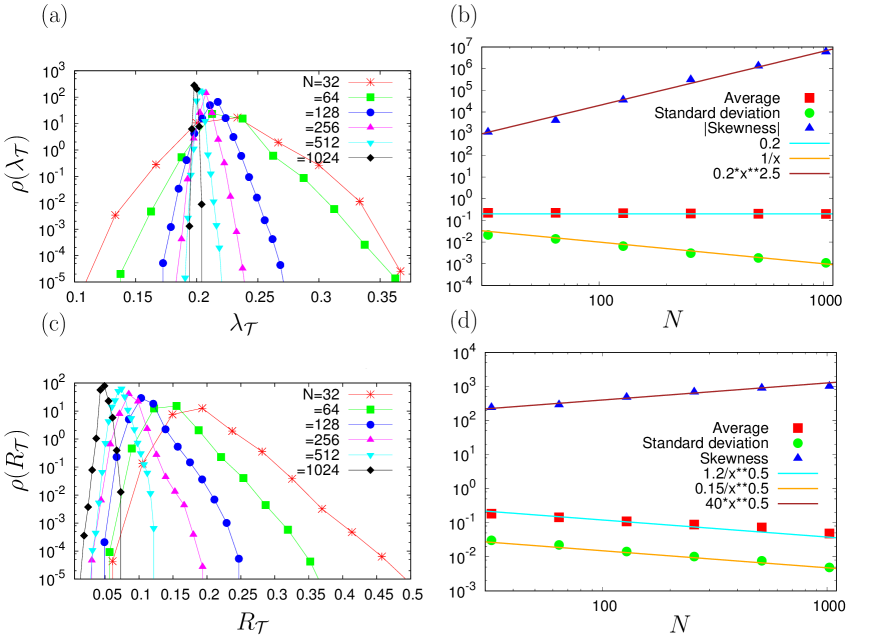
Figure 2: (Color online) Non-trivial scaling with $N$ of two observables in the HMF model. (a) Distribution of the FTLE $\lambda_{\cal T}$ (with ${\cal T}=10.0$) and (b) variation of the mean, the standard deviation, and the skewness with the number $N$ of oscillators. (c) Distribution of the TASOP $R_{\cal T}$ (with ${\cal T}=10.0$) and (d) variation of the mean, the standard deviation, and the skewness with the number of oscillators. The results correspond to the HMF model (3) with coupling constant $K=1$ and energy density $\epsilon=2.0$, and are obtained by performing independent simulations with several different values of $\beta$ chosen suitably for each $N$, and combining the results so obtained; in each case, several thousand data points have been collected. For the FTLE $\lambda_{\cal T}$, we propose and accept states using $O_{\cal T}=\lambda_{\cal T}$ in the algorithm given in Sections III.2 and III.3. For the TASOP $R_{\cal T}$, however, we propose states using $O_{\cal T}=\lambda_{\cal T}$ in the algorithm given in Section III.2, and accept states using $O_{\cal T}=R_{\cal T}$ in Section III.3.

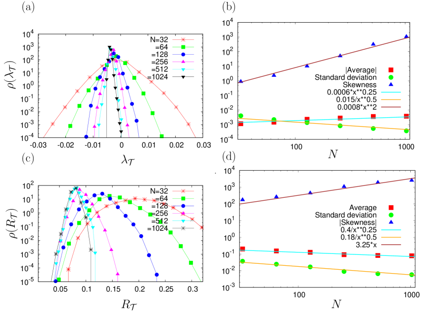
Figure 3: (Color online) Non-trivial scaling with $N$ of two observables in the Kuramoto model. (a) Distribution of the FTLE $\lambda_{\cal T}$ (with ${\cal T}=10.0$) and (b) variation of the mean, the standard deviation, and the skewness with the number of oscillators $N$. (c) Distribution of the TASOP $R_{\cal T}$ (with ${\cal T}=10.0$) and (d) variation of the mean, the standard deviation, and the skewness with the number $N$ of oscillators. The results correspond to the Kuramoto model (4) with the natural frequencies taken to be Gaussian distributed with zero mean and unit variance, yielding $\widetilde{K}_{c}=2\sqrt{2/\pi}\approx 1.6$; here, we have $\widetilde{K}=0.25$. The results are obtained by performing independent simulations with several different values of $\beta$ chosen suitably for each $N$, and then combining the results so obtained; in each case, several thousand data points have been collected. For the FTLE $\lambda_{\cal T}$, we propose and accept states using $O_{\cal T}=\lambda_{\cal T}$ in the algorithm given in Sections III.2 and III.3. For the TASOP $R_{\cal T}$, however, we propose states using $O_{\cal T}=\lambda_{\cal T}$ in the algorithm given in Section III.2, and accept states using $O_{\cal T}=R_{\cal T}$ in Section III.3.

The results for the HMF model are shown in Fig. 2. The distributions of both the observables ($\lambda_{\cal T}$ and $R_{\cal T}$) become narrower with increasing $N$, suggesting a convergence to a single value as $N\rightarrow\infty$. To further quantify this (expected) behaviour, we investigate the $N$-dependence of the first three standardized moments of the distributions (i.e., the mean, the standard deviation, and the skewness). It is essential to employ our algorithm in the estimation of high moments because of their values being increasingly sensitive to the tails of the distribution.

Let us now discuss in more detail the interpretation of the results shown in Fig. 2. They provide valuable insights into the properties of the equilibrium dynamics of the HMF model that are hard to obtain analytically due to the highly non-linear and complex nature of the dynamics. Since we are at an energy higher than the critical value $\epsilon_{c}$, the system is in an unmagnetized and chaotic steady state, implying that one has $\lambda_{{\cal T}\rightarrow\infty}>0$ and $\langle R_{1}\rangle=0$ in the thermodynamic limit $N\to\infty$. From panel (a), we see here that with increase of $N$, the typical or the most probable value of $\lambda_{\cal T}$ tends towards a positive value, confirming that typical regions of the HMF model phase space are characterized by chaotic trajectories, that is, trajectories that while starting close together diverge from one another exponentially fast. The results for the parameter $R_{\cal T}$, reported in panels (c) and (d), show that the typical value of $R_{\cal T}$ tends towards zero with increase of $N$, confirming that in the large-$N$ limit, a typical state of the system in equilibrium is unmagnetized, and during the dynamics, the chaotic trajectories pass through sequences of states that too are unmagnetized, being different from one another in the distribution of the points depicting the phases of the oscillators. The main new result shown in the figure is that, even for large $N$, atypical states with values of observables different from the typical value are observed, as reflected by the increase in the magnitude of the skewness with system size $N$ (the topmost plot in panels (b) and (d)). This is observed not only for $R_{\cal T}$, for which $\langle R_{\cal T}\rangle\rightarrow 0$ with increase of $N$ and $R_{\cal T}$ as a physical quantity satisfies $R_{\cal T}\geq 0$ , but also for $\lambda_{\cal T}$, which means that for finite $N$, there are a significant number of atypical states that during the dynamics exhibit a different chaoticity and a larger magnetization than the typical states.

Figure 3 shows that the results discussed above are observed also in the Kuramoto model. This is significant because it shows that our observations are valid for both first- and second-order systems and in both conservative and dissipative dynamics. Note that the parameter values for which we investigated the Kuramoto model were such that the model has an unsynchronized and chaotic stationary state, being therefore in a steady state similar to the equilibrium state of the HMF model discussed in Fig. 2.

On the basis of the foregoing discussions, we thus arrive at an important conclusion regarding the dynamics of coupled oscillators, be it conservative as in the HMF model or dissipative as in the Kuramoto model, that stationary-state fluctuations do not die down but remain significant even for large $N$, and that one tail of the distribution is particularly prominent with respect to the other one. While it is definitely of urgent interest to explain analytically the different scalings with $N$ observed in the behavior of the moments in Figs. 2 and 3, a roadblock is the fact that for $N$ as large as $1024$, the dynamical trajectories of the oscillators in both the HMF model and the Kuramoto model do not evolve independently of one other, but remain strongly coupled in time.

Finally, we quantify the efficiency of our method. To this end, the crucial element is the correlation of the sequence of data points generated by our Monte Carlo algorithm Newman:2002 , or, in other words, the number of steps the algorithm needs to obtain independent samples. The details of estimating this correlation time from the generated data are described in Appendix C. The results for the autocorrelation are reported in Fig. 4. A particularly revealing and important observation that may be made from the figure is that the correlation time does not (substantially) increase with increasing $N$. This fact is further corroborated by our results on the integrated correlation time reported in Table 1, which should be compared with traditional (uniform sampling) method where the integrated correlation time is expected to grow exponentially with $N$.

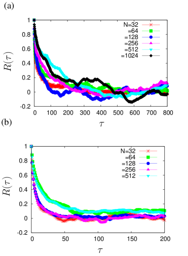
Figure 4: Autocorrelation $R(\tau)$, defined in Eq. (28), for the HMF model. Panel (a) is for the FTLE $\lambda_{\cal T}$, while panel (b) is for the TASOP $R_{\cal T}$. The coupling constant is $K=1$, the energy density is $\epsilon=2.0$, while we have taken ${\cal T}=10.0$.

$N$	$\mathscr{T}$
$32$	$0.033$
$64$	$0.055$
$128$	$0.051$
$256$	$0.081$
$512$	$0.112$
1024	$0.113$

$N$	$\mathscr{T}$
$32$	$0.024$
$64$	$0.050$
$128$	$0.029$
$256$	$0.025$
$512$	$0.043$
$1024$	0.19

Table 1: Integrated autocorrelation $\mathscr{T}$ (see Eq. (29)) corresponding to Fig. 4, with the left (right) table corresponding to the panel (a) (panel (b)) of Fig. 4.

V Conclusions and perspectives

In this work, we investigated the variability in the behavior of dynamical trajectories due to different initial conditions in systems of coupled oscillators, by developing dedicated numerical algorithms particularly suited to study rare events in non-linear complex dynamics of many-body dynamical systems. We focused on two representative observables, namely, the finite-time Lyapunov exponent and a time-averaged order parameter. With increase of the system size $N$, the distribution of such observables becomes increasingly peaked around the value obtained in the limit $N\rightarrow\infty$, thereby making it extremely hard to characterize for large $N$ the shape of the distribution away from this value, with the associated computational cost using traditional (uniform sampling) methods increasing dramatically (typically exponentially) with $N$. Here, to show the generality of our algorithm, we studied two paradigmatic systems with contrasting dynamics, namely, the equilibrium, second-order, conservative dynamics of the Hamiltonian mean-field model, and the non-equilibrium, first-order, dissipative dynamics of the Kuramoto model. We performed simulations over a wide range of system size, from $N=32$ to $N$ as large as $1024$. Our algorithm, based on a Metropolis-Hastings Monte Carlo Method Newman:2002 applied earlier for low-dimensional chaotic systems Leitao:2017 , contains crucial adaptations necessary to deal with coupled oscillators (e.g., extension to continuous-time dynamics and modification of the way states are proposed). Our numerical results confirm the accuracy (Fig. 1) and efficiency (Fig. 4 and Table 1) of our method.

Our main numerical finding is the non-trivial convergence in the limit $N\rightarrow\infty$ of the distribution $\rho(O_{\cal T})$ to the asymptotic form. In particular, we found in all the cases of study, namely, for the two observables in the two contrasting dynamics, that the magnitude of the skewness of the distribution grows with $N$. This implies the relative importance of one tail of the distribution over the other with increase of $N$, despite reduced fluctuations (i.e., with the standard deviation $\to 0$). These observations suggest that even for large $N$, states yielding values of observables substantially deviated from the typical value occur with significant probabilities. To understand theoretically the scaling of the different moments with $N$ observed in Figs. 2 and 3 is a particularly challenging task left for future studies.

The successful application of our method demonstrated in this work suggests the exciting possibility to apply our algorithm to more complex dynamics, e.g., to investigate the properties of the out-of-equilibrium quasi-stationary states Campa:2014 in the HMF model, the subtle dependence of the dynamics on the realizations of the natural frequencies $\omega_{i}$’s in the Kuramoto model, the existence of the so-called chimera states Panaggio:2015 in oscillator systems in which they appear, and also in determining the distribution of Lyapunov exponents in other relevant long-range systems such as the self-gravitating ring model Tatekawa:2015 .

VI Acknowledgements

SG acknowledges fruitful discussions with T. Manos, A. Politi, and S. Ruffo. JL acknowledges funding from grant SFRH/BD/90050/2012 (FCT Portugal) and fruitful discussions with J. V. Parente Lopes.

Appendix A Observables: The FTLE $\lambda_{\cal T}$ and the TASOP $R_{\cal T}$

A.1 The finite-time Lyapunov exponent $\lambda_{\cal T}$ (FTLE)

We define here the FTLE $\lambda_{\cal T}$ corresponding to the dynamics (1). The definition may be suitably modified for the HMF and the Kuramoto model by taking the appropriate limits of the dynamics discussed in Section II. Let ${\bf r}(t)$ denote a state of the system at time $t$, and let $\{{\bf r}(\tau);~{}\tau\in[0,{\cal T}]\}$ be the trajectory obtained by evolving a given initial state for time ${\cal T}$ according to the dynamics of ${\bf r}(t)$. Here, ${\bf r}(t)$ is the $2N$-dimensional vector of phases and angular velocities of the $N$ oscillators: $r_{1,2,\ldots,N}=\theta_{i=1,2,\ldots,N}$ and $r_{N+1,N+2,\ldots,2N}=v_{i=1,2,\ldots,N}$. Corresponding to the dynamics

$$\frac{{\rm d}{\bf r}(t)}{{\rm d}t}={\bf F}({\bf r}(t)),$$ (14)

a set of infinitesimal displacements $\{\delta r_{i}(t)\}$ from a given phase space point ${\bf r}(t)$ at time $t$ will have its evolution described by the following linearized equations of motion:

$$\delta r_{i}(t)=\sum_{j=1}^{2N}\frac{{\rm d}{F}_{i}}{{\rm d}r_{j}}\Big{|}_{{\bf r}(t)}\delta r_{j}(t);~{}~{}i,j=1,2,\ldots,2N,$$ (15)

where the elements $\frac{{\rm d}F_{i}}{{\rm d}r_{j}}\Big{|}_{{\bf r}(t)}$ define the Jacobian matrix $J_{ij}$ evaluated at ${\bf r}(t)$. For the dynamics (1), one has

$$F_{i}=\left\{\begin{array}[]{ll}r_{i+N}\mbox{~{}for $1\leq i\leq N$},&\\ \gamma(\omega_{i-N}-r_{i})/m+(K/m)\sum_{s=1}^{\infty}s\widetilde{u}_{s}\Big{[}-R^{(x)}_{s}\sin(sr_{i-N})+R^{(y)}_{s}\cos(sr_{i-N})\Big{]}&\\ \mbox{~{}for $N+1\leq i\leq 2N$},&\\ \end{array}\right.$$ (18)

$$J_{ij}=\left\{\begin{array}[]{ll}1\mbox{~{}for $1\leq i\leq N,N+1\leq j\leq 2N$},&\\ -(K/(Nm))\sum_{s=1}^{\infty}s\widetilde{u}_{s}\cos(s(r_{i-N}-r_{j}))\mbox{~{}for $N+1\leq i\leq 2N,1\leq j\leq N,i\neq j$},&\\ (K/m)\sum_{s=1}^{\infty}s\widetilde{u}_{s}\Big{(}R^{(x)}_{s}\cos(sr_{j})+R^{(y)}_{s}\sin(sr_{j})-\frac{1}{N}\Big{)}\mbox{~{}for $N+1\leq i\leq 2N,1\leq j\leq N,i=j$},&\\ 0\mbox{~{}otherwise}.&\end{array}\right.$$ (23)

Starting with a given set $\{{\bf r}(t),\delta{\bf r}(t)\}$ at time $t$, and evolving under Eqs. (14) and (15) for a total time ${\cal T}$, the FTLE $\lambda_{\cal T}$ is defined as

$$\lambda_{\cal T}({\bf r}(t))\equiv\frac{1}{{\cal T}}\log\frac{d(t+{\cal T})}{d(t)},$$ (25)

with $d(t)\equiv\sqrt{\sum_{i=1}^{2N}[\delta r_{i}(t)]^{2}}$ the metric distance calculated from the infinitesimal displacements measured from the instantaneous location ${\bf r}(t)$ at time $t$. The FTLE $\lambda_{\cal T}$ is thus a measure of the finite-time (i.e., in time ${\cal T}$) exponential divergence of different trajectories starting close to ${\bf r}(t)$ at time $t$.

We used the following algorithm to efficiently compute $\lambda_{\cal T}$. The starting point is the generation of the perturbations $\delta r_{i}$ for $i=1,2,\ldots,N_{\rm tot}$; the obtained values are then scaled as $\delta r_{i}\to\delta r_{i}/d$, with $d\equiv\Big{(}\sum_{i=1}^{N_{\rm tot}}(\delta r_{i})^{2}\Big{)}^{1/2}$. Starting with the given set $\{r_{i}\}$ and $\{\delta r_{i}\}$, their values are evolved in time Integrator according to the equations of motion of the model at hand for a total time ${\cal T}$, by computing at every time interval $\tau$ the quantity $d_{\alpha}\equiv\Big{(}\sum_{i=1}^{N_{\rm tot}}(\delta r_{i}^{(\alpha)})^{2}\Big{)}^{1/2},$ with $\alpha=1,2,\ldots,{\cal T}/\tau,$ and by rescaling the perturbations as $\delta r_{i}^{(\alpha)}\to\delta r_{i}^{(\alpha)}/d_{\alpha}$. Here, $N_{\rm tot}$ is the total number of degrees of freedom: $N_{\rm tot}=2N$. Then $\lambda_{\cal T}$ is estimated as

$$\lambda_{\cal T}({\bf r}) \equiv\frac{1}{{\cal T}}\sum_{\alpha=1}^{{\cal T}/\tau}\ln d_{\alpha}.$$ (26)

A.2 The time-averaged synchronization order parameter $R_{\cal T}$ (TASOP)

A time evolution for time ${\cal T}$ while starting from a given phase space point ${\bf r}(t)$ yields the time-averaged synchronization order parameter $R_{\cal T}$ (TASOP) defined as

$$R_{s,{\cal T}}({\bf r}(t))\equiv\frac{1}{{\cal T}}\int_{t}^{t+{\cal T}}{\rm d}t^{\prime}~{}||\Big{(}R^{(x)}_{s}(t^{\prime}),R^{(y)}_{s}(t^{\prime})\Big{)}||,$$ (27)

with $||(x,y)||\equiv\sqrt{x^{2}+y^{2}}$, and $R^{(x),(y)}_{s}(t^{\prime})$ corresponding to the phase space point ${\bf r}(t^{\prime})$ is defined in Eq. (5). In this work, we will specifically consider $R_{\cal T}({\bf r}(t))\equiv R_{1,{\cal T}}({\bf r}(t))$. Note that $R_{\cal T}$ is a positive quantity: $R_{\cal T}\geq 0$.

Appendix B Preparation of the initial state ${\bf r}\equiv\{\theta_{i},v_{i}\}$ with fixed energy density $\epsilon$ and net momentum zero for the HMF model

The relevant steps are

1. Assign independently for $i=1,2,\ldots,N$ the $\theta_{i}$’s as $\theta_{i}\sim U[0,2\pi]$.

2. Compute the potential energy $V(\{\theta_{i}\})=\frac{K}{2N}\sum_{i,j=1}^{N}[1-\cos(\theta_{i}-\theta_{j})]$, and thence the allowed value of the kinetic energy per oscillator for the given realization of the $\theta_{i}$’s as $T_{{\rm allowed}}(\{\theta_{i}\})\equiv\epsilon-V(\{\theta_{i}\})/N$.

3. Assign independently for $i=1,2,\ldots,N$ the angular velocities $v_{i}$’s as $v_{i}\sim\sqrt{2T_{{\rm allowed}}((\theta_{i}\})}\mathcal{N}(0,1)$. In this way, $\sum_{i=1}^{N}v_{i}$ is very close to zero (with corrections that decrease with increasing $N)$, but is not exactly so, and also $\sum_{i=1}^{N}v_{i}^{2}/2$ is very close to the allowed value $NT_{{\rm allowed}}(\{\theta_{i}\})$ of the kinetic energy (with corrections that decrease with increasing $N)$, but is not exactly so.

4. Compute the average velocity $v_{\rm avg}\equiv\sum_{i=1}^{N}v_{i}/N,$ and transform for $i=1,2,\ldots,N$ the $v_{i}$’s as $v_{i}\to v^{\prime}_{i}=v_{i}-v_{\rm avg},$ thereby ensuring that $\sum_{i=1}^{N}v^{\prime}_{i}=0$. From now on, let us drop the prime for notational convenience.

5. Compute the actual kinetic energy $T_{{\rm actual}}(\{\theta_{i},v_{i}\})$ for the set of $v_{i}$’s at hand, while we already have the value of the potential energy $V(\{\theta_{i}\})$ from step 2. We then compute the quantity $\alpha\equiv\sqrt{|N\epsilon-V(\{\theta_{i}\})|/T_{{\rm actual}}(\{\theta_{i},v_{i}\})}$.

6. Scale for $i=1,2,\ldots,N$ the $v_{i}$’s as $v_{i}^{\prime}\equiv\alpha v_{i}$. This ensures that $\sum_{i=1}^{N}v_{i}^{2}/2=N\epsilon-V(\{\theta_{i}\})=NT_{{\rm allowed}}(\{\theta_{i}\})$, as desired.

Appendix C Efficiency of the algorithm

The efficiency of our algorithm depends critically on the correlation time of the generated sequence of the values of the observable, which may be quantified as follows. For a given $N$, the distribution of $O_{\cal T}$ obtained by uniform sampling gives an estimate of the most probable value $O^{\rm mp}_{\cal T}$. We then choose a value $O^{\rm tail}_{\cal T}$ of $O_{\cal T}$ on the tail, say, at a distance $2\sigma$ from $O^{\rm mp}_{\cal T}$, where $\sigma$ is the standard deviation of the distribution of $O_{\cal T}$. We then employ the importance sampling scheme detailed in the paper to obtain a time series $\{O_{\cal T}^{(i)}\}_{1\leq i\leq M}$ and thence, a biased distribution centered around $O^{\rm tail}_{\cal T}$. Next, knowing the full width at half maximum of the biased distribution, we define an indicator variable $I_{i}$ that takes the value of unity provided the $i$-th value $O_{\cal T}^{(i)}$ lies within the full width and takes the value zero otherwise. The autocorrelation is then computed as

$$R(\tau)\equiv\frac{\sum_{i=1}^{M-\tau}\Big{(}I_{i}-\overline{I}\Big{)}\Big{(}I_{i+\tau}-\overline{I}\Big{)}}{(M-\tau)\sigma_{I}^{2}};~{}~{}0\leq\tau\leq\frac{M}{2},$$ (28)

where $\overline{I}\equiv\frac{1}{M}\sum_{i=1}^{M}I_{i},$ and $\sigma_{I}^{2}\equiv\frac{1}{M}\sum_{i=1}^{M}(I_{i}-\overline{I})^{2}$. The integrated autocorrelation is defined as

$$\mathscr{T}\equiv\frac{2}{M}\sum_{\tau=1}^{M/2}|R(\tau)|.$$ (29)

References

- (1) The Fermi-Pasta-Ulam problem: A status report, edited by G. Gallavotti (Springer-Verlag, Berlin, 2007).
- (2) Hamiltonian Dynamical Systems: a reprint selection, edited by R. S. MacKay and J. D. Meiss (Adam Hilger, Bristol, 1987).
- (3) T. Komatsuzaki and R. S. Berry, Adv. Chem. Phys. 123, 79 (2002).
- (4) S. H. Strogatz, Nonlinear Dynamics And Chaos: With Applications To Physics, Biology, Chemistry, And Engineering (Westview Press, Boulder, 2014).
- (5) M. E. J. Newman and G. T. Barkema, Monte Carlo Methods in Statistical Physics (Oxford University, New York, 2002).
- (6) J. Tailleur and J. Kurchan, Nat. Phys. 3, 203 (2007).
- (7) J. C. Leitão, J. M. V. P. Lopes and E. G. Altmann, arXiv:1701.06265 (2017).
- (8) In presence of a finite moment of inertia, an oscillator is more traditionally referred to as a rotor; here, however, we continue to refer to it as an oscillator.
- (9) A. Campa, T. Dauxois and S. Ruffo, Phys. Rep. 480, 57 (2009).
- (10) F. Bouchet, S. Gupta and D. Mukamel, Physica A 389, 4389 (2010).
- (11) A. Campa, T. Dauxois, D. Fanelli and S. Ruffo, Physics of Long-range Interacting Systems (Oxford University Press, UK, 2014).
- (12) S. Gupta and S. Ruffo, Int. J. Mod. Phys. A 32, 1741018 (2017) (Special Issue on the occasion of Abdus Salam’s 90th Birthday).
- (13) This ensures that the internal torque on the -th oscillator due to the -th one is balanced by that on the -th oscillator due to the -th one.
- (14) M. Antoni and S. Ruffo, Phys. Rev. E 52, 2361 (1995).
- (15) T. Dauxois, V. Latora, A. Rapisarda, S. Ruffo and A. Torcini, in Dynamics and Thermodynamics of Systems with Long Range Interactions, Lecture Notes in Physics Volume 602, edited by T. Dauxois, S. Ruffo, E. Arimondo and M. Wilkens (Springer, Berlin, 2002).
- (16) Y. Kuramoto, International Symposium on Mathematical Problems in Theoretical Physics, Lecture Notes in Physics, Vol. 39 edited by H Araki (Springer, New York, 1975).
- (17) Y. Kuramoto, Chemical oscillations, Waves and Turbulence (Springer, Berlin, 1984).
- (18) S. H. Strogatz, Physica D 143, 1 (2000).
- (19) A. Pikovsky, M. Rosenblum and J. Kurths, Synchronization: A Universal Concept in Nonlinear Sciences (Cambridge University Press, Cambridge, 2001).
- (20) J. A. Acebrón, L. L. Bonilla, C. J. P. Vicente, F. Ritort and R. Spigler, Rev Mod Phys 77, 137 (2005).
- (21) S. H. Strogatz, Sync: The Emerging Science of Spontaneous Order (Hyperion, New York, 2003).
- (22) S. Gupta, A. Campa and S. Ruffo, J. Stat. Mech.: Theory Exp. R08001 (2014).
- (23) A. Pikovsky and A. Politi, Lyapunov Exponents: A Tool to Explore Complex Dynamics (Cambridge University Press, Cambridge, 2016).
- (24) V. Latora, A. Rapisarda and S. Ruffo, Phys. Rev. Lett. 80, 692 (1998).
- (25) M.-C. Firpo, Phys. Rev. E 57, 6599 (1998).
- (26) V. Latora, A. Rapisarda and S. Ruffo, Physica D 131, 38 (1999).
- (27) T. Manos and S. Ruffo, Transport Theory and Statistical Physics 40, 360 (2011).
- (28) L. H. Miranda Filho, M. A. Amato and T. M. Rocha Filho, arXiv:1704.02678.
- (29) F. Ginelli, K. A. Takeuchi, H. Chaté, A. Politi and A. Torcini, Phys. Rev. E 84, 066211 (2011).
- (30) G. Radons, in Collective Dynamics of Nonlinear and Disordered Systems, edited by G. Radons, W. Just, and P. Häussler (Springer-Verlag, Berlin, 2005).
- (31) O. V. Popovych, Y. L. Maistrenko and P. A. Tass, Phys. Rev. E 71, 065201(R) (2005).
- (32) This value may be easily estimated by performing a simulation.
- (33) A Guide to Monte Carlo Simulations in Statistical Physics by D. P. Landau and K. Binder (Cambridge University Press, UK, 2014).
- (34) M. J. Panaggio and D. M. Abrams, Nonlinearity 28, R67 (2015).
- (35) T. Tatekawa, F. Bouchet, T. Dauxois and S. Ruffo, Phys. Rev. E 71, 056111 (2005).
- (36) In the case of energy-conserving HMF dynamics, we use a fourth-order symplectic integrator McLachlan:1992 to integrate the equations of motion; in the case of the dissipative Kuramoto dynamics, we use instead a fourth-order Runge-Kutta scheme.
- (37) R. I. McLachlan and P. Atela, Nonlinearity 5, 541 (1992).