Using infinite volume, continuum QED and lattice QCD for the hadronic light-by-light contribution to the muon anomalous magnetic moment

Abstract

In Ref Blum:2016lnc , the connected and leading disconnected hadronic light-by-light contributions to the muon anomalous magnetic moment ($g-2$) have been computed using lattice QCD ensembles corresponding to physical pion mass generated by the RBC/UKQCD collaboration. However, the calculation is expected to suffer from a significant finite volume error that scales like $1/L^{2}$ where $L$ is the spatial size of the lattice. In this paper, we demonstrate that this problem is cured by treating the muon and photons in infinite volume, continuum QED, resulting in a weighting function that is pre-computed and saved with affordable cost and sufficient accuracy. We present numerical results for the case when the quark loop is replaced by a muon loop, finding the expected exponential approach to the infinite volume limit and consistency with the known analytic result. We have implemented an improved weighting function which reduces both discretization and finite volume effects arising from the hadronic part of the amplitude.

I Introduction

Precision measurements of lepton magnetic dipole moments provide a powerful tool to test the standard model (SM) of particle physics at high precision. The magnetic dipole moment $\vec{\mu}$ originating from the lepton’s spin $\vec{s}$ is commonly expressed as

$$\vec{\mu}=g\left(\frac{e}{2m}\right)\vec{s}\,,$$ (1)

where $e$ is the lepton’s electromagnetic charge and $m$ is its mass. The anomalous magnetic moment, or anomaly, $a=(g-2)/2$ expresses the deviation from Dirac’s relativistic quantum-mechanical prediction $g=2$. It is generated by small radiative corrections which by a careful comparison between its experimental measurement to its theory prediction may reveal physics beyond the standard model. Experimental measurements have determined these anomalous moments at very high precision. The electron anomaly, $a_{e}=0.00115965218073(28)$ Hanneke:2008tm , currently yields the most precise value of the fine structure constant $\alpha=1/137.035999157(33)$ Aoyama:2014sxa . In general, contributions from a new physics scale $\Lambda_{\rm NP}$ to the anomalous magnetic moment of a lepton $\ell=e,\mu,\tau$ are suppressed by $m^{2}_{\ell}/\Lambda^{2}_{\rm NP}$. One therefore expects the muon to be five orders of magnitude more sensitive to such contributions than the electron which outweighs a loss in experimental precision. With the $\tau$ being experimentally inaccessible, $a_{\mu}$ is the most promising channel to reveal physics beyond the standard model.

Interestingly, current experimental and theoretical determinations of $a_{\mu}$ differ at the $3.1$–$3.5$ standard deviation level,

$$a_{\mu}^{\rm EXP}-a_{\mu}^{\rm SM}=\,\, (27.6\pm 8.0)\times 10^{-10}\leavevmode\nobreak\ \text{\cite[cite]{\@@bibref{Authors Phrase1YearPhrase2}{Davier:2010nc}{\@@citephrase{(}}{\@@citephrase{)}}}}\,,$$

$$(25.0\pm 8.0)\times 10^{-10}\leavevmode\nobreak\ \text{\cite[cite]{\@@bibref{Authors Phrase1YearPhrase2}{Hagiwara:2011af}{\@@citephrase{(}}{\@@citephrase{)}}}}\,,$$ (2)

depending on which value for the hadronic vacuum polarization contribution is used (see Tab. 1).

Contribution	Value $\times 10^{10}$	Uncertainty $\times 10^{10}$
QED	11 658 471.895	0.008
Electroweak Corrections	15.4	0.1
HVP (LO) Davier:2010nc	692.3	4.2
HVP (LO) Hagiwara:2011af	694.9	4.3
HVP (NLO)	-9.84	0.06
HVP (NNLO)	1.24	0.01
HLbL	10.5	2.6
Total SM prediction Davier:2010nc	11 659 181.5	4.9
Total SM prediction Hagiwara:2011af	11 659 184.1	5.0
BNL E821 result	11 659 209.1	6.3
Fermilab E989 target		$\approx$ 1.6

Table 1: Individual contributions to the current standard model calculation of $a_{\mu}$ PDG2013 ; Kurz:2014wya . The BNL E821 experimental result Bennett:2006fi and Fermilab E989 target precision Grange:2015fou are given for comparison.

In this tension the theory and experimental uncertainties are approximately balanced, with the theory uncertainty dominated by the hadronic vacuum polarization and hadronic light-by-light (HLbL) contributions. With future experiments at Fermilab (E989) Carey:2009zzb and J-PARC (E34) Aoki:2009xxx aiming for a four-fold decrease in experimental uncertainty, a careful first-principles determination of these hadronic contributions and a similar reduction in uncertainty is desirable.

In this work we present an improved method to compute the HLbL contribution from first principles in lattice quantum chromodynamics (QCD). We build on the optimized sampling strategy of the HLbL diagrams, which we have introduced in Ref. Blum:2015gfa and which has reduced the statistical uncertainties, at the same cost, by more than an order of magnitude compared to the pioneering work of Ref. Blum:2014oka . In a recent publication Blum:2016lnc , we have presented a first-principles 2+1 flavor lattice QCD calculation of the connected and leading disconnected contributions to the muon anomaly at physical quark and muon masses,

$$a_{\mu}^{\rm HLbL} =5.35(1.35)\times 10^{-10}\,,$$ (3)

where the statistical uncertainty is given. This result is affected by potentially large systematic errors due to the non-zero lattice spacing and the finite lattice volume used in our calculation. We are in the process of repeating our calculation on a second lattice spacing to address the former systematic. The latter is addressed in this work.

So far all lattice QCD calculations of the HLbL contribution to the muon $g-2$ have treated the photons and muon in the same finite hypercubic lattice where the quarks and gluons live. The results are expected to suffer from sizable finite volume corrections which scale as some power of the system size rather than the exponential scaling observed for typical lattice QCD calculations since the photons are restricted to a finite box. Inspired by earlier work on the hadronic vacuum polarization Blum:2002ii , we remove power-law finite volume errors by computing the muon and photon components of our diagrams in infinite volume and subsequently combine the resulting weight function with a QCD four-point function obtained in our lattice simulation. The Mainz group announced a similar approach Asmussen:2016lse ; Green:2015sra , which, to a large extent, motivated this work.

In the following we describe our method in detail and verify it in the leptonic case, where we replace the quark by a lepton loop. This replacement is trivial from the perspective of our lattice calculation and the same setup with free propagators replaced by propagators on a non-trivial QCD background allows us to perform the calculation in the desired QCD case.

In Ref Blum:2015gfa , we introduced a formula to obtain the connected hadronic light-by-light contribution to the anomalous magnetic moment given by the electromagnetic Pauli form factor evaluated at zero momentum transfer, $F_{2}(q^{2}=0)$, from a lattice calculation:

$$\frac{F_{2}^{\operatorname{cHLbL}}(q^{2}=0)}{m}\frac{(\sigma_{s^{\prime},s})_{i}}{2} = \frac{1}{VT}\sum_{x,y,z}\sum_{x_{\text{op}}}\frac{1}{2}\epsilon_{i,j,k}\left(x_{\text{op}}-x_{\operatorname{ref}}\right)_{j}\cdot i\bar{u}_{s^{\prime}}(\vec{0})\mathcal{F}^{C}_{k}\left(x,y,z,x_{\text{op}}\right)u_{s}(\vec{0}),$$ (4)

where $(\sigma_{s^{\prime},s})_{i}=\bar{u}_{s^{\prime}}(\vec{0})\Sigma_{i}u_{s}(\vec{0})$ are the conventional Pauli matrices. The coordinates $x_{\text{op}},\leavevmode\nobreak\ x,\leavevmode\nobreak\ y,\leavevmode\nobreak\ z$ are the locations of the electromagnetic currents on the quark loop, the former corresponding to the external photon and the latter to the virtual photons connecting the quark loop to the muon (see Fig. 1). The point $x_{\operatorname{ref}}$ can be chosen arbitrarily and may even depend on $x$, $y$, and $z$. In Ref Blum:2015gfa , we set $x_{\operatorname{ref}}=(x+y)/2$ and further manipulated the above formula to take advantage of the symmetry between $x$, $y$, $z$ to reduce the statistical noise inherent in our monte carlo integration:

$$\frac{F_{2}^{\operatorname{cHLbL}}(q^{2}=0)}{m}\frac{(\sigma_{s^{\prime},s})_{i}}{2} = \sum_{r,\tilde{z}}\mathfrak{Z}\left(\frac{r}{2},-\frac{r}{2},\tilde{z}\right)\sum_{\tilde{x}_{\text{op}}}\frac{1}{2}\epsilon_{i,j,k}\left(\tilde{x}_{\text{op}}\right)_{j}\cdot i\bar{u}_{s^{\prime}}(\vec{0})\mathcal{F}^{C}_{k}\left(\frac{r}{2},-\frac{r}{2},\tilde{z},\tilde{x}_{\text{op}}\right)u_{s}(\vec{0}).$$ (5)

The integration variables are related to the coordinates in Fig. 1 by the following equations: $r=x-y$, $\tilde{z}=z-(x+y)/2$, $\tilde{x}_{\text{op}}=x_{\text{op}}-(x+y)/2$. The function “$\mathfrak{Z}$” is defined by

$$\mathfrak{Z}(x,y,z) = \left\{\begin{array}[]{ll}3&\text{if }|x-y|<|x-z|\text{ and }|x-y|<|y-z|\\ 3/2&\text{if }|x-y|=|x-z|<|y-z|\text{ or }|x-y|=|y-z|<|x-z|\\ 1&\text{if }|x-y|=|x-z|=|y-z|\\ 0&\text{otherwise}\end{array}\right..$$ (10)

We compute the summation over $r$ in Eq. (5) by stochastically sampling $x$ and $y$ point pairs, while the sums over $\tilde{x}_{\text{op}}$ and $\tilde{z}$ are performed completely over the entire lattice. The amplitude $\mathcal{F}^{C}_{\nu}\left(x,y,z,x_{\text{op}}\right)$ is given by:

$$\mathcal{F}^{C}_{\nu}\left(x,y,z,x_{\text{op}}\right) = (-ie)^{6}\mathcal{G}_{\rho,\sigma,\kappa}(x,y,z)\mathcal{H}^{C}_{\rho,\sigma,\kappa,\nu}(x,y,z,x_{\operatorname{op}}),$$ (11)

where $i^{4}\mathcal{H}^{C}_{\rho,\sigma,\kappa,\nu}(x,y,z,x_{\operatorname{op}})$ represents the four-point hadronic correlation function, and $i^{3}\mathcal{G}_{\rho,\sigma,\kappa}(x,y,z)$ is the QED weighting function. For the connected diagram, $i^{4}\mathcal{H}^{C}_{\rho,\sigma,\kappa,\nu}(x,y,z,x_{\operatorname{op}})$ is given by the following two equations:

$$i^{4}\mathcal{H}^{C}_{\rho,\sigma,\kappa,\nu}(x,y,z,x_{\operatorname{op}}) = \frac{1}{6}\mathcal{H}_{\rho,\sigma,\kappa,\nu}(x,y,z,x_{\operatorname{op}})+\frac{1}{6}\mathcal{H}_{\sigma,\kappa,\rho,\nu}(y,z,x,x_{\operatorname{op}})+\frac{1}{6}\mathcal{H}_{\kappa,\rho,\sigma,\nu}(z,x,y,x_{\operatorname{op}})$$

$$+\frac{1}{6}\mathcal{H}_{\kappa,\sigma,\rho,\nu}(z,y,x,x_{\operatorname{op}})+\frac{1}{6}\mathcal{H}_{\rho,\kappa,\sigma,\nu}(x,z,y,x_{\operatorname{op}})+\frac{1}{6}\mathcal{H}_{\sigma,\rho,\kappa,\nu}(y,x,z,x_{\operatorname{op}}),$$

$$\mathcal{H}_{\rho,\sigma,\kappa,\nu}(x,y,z,x_{\operatorname{op}}) = \sum_{q=u,d,s}(e_{q}/e)^{4}\left\langle-\operatorname{tr}\left[i\gamma_{\rho}S_{q}(x,z)i\gamma_{\kappa}S_{q}(z,y)i\gamma_{\sigma}S_{q}\left(y,x_{\text{op}}\right)i\gamma_{\nu}S_{q}\left(x_{\text{op}},x\right)\right]\right\rangle_{\text{QCD}},$$ (13)

where $e_{u}/e=2/3$, and $e_{d}/e=e_{s}/e=-1/3$. The QED weighting function, $i^{3}\mathcal{G}_{\rho,\sigma,\kappa}(x,y,z)$, is a symmetrized version of $\mathfrak{G}_{\sigma,\kappa,\rho}(y,z,x)$, which is represented by the right diagram of Fig. 1:

$$i^{3}\mathcal{G}_{\rho,\sigma,\kappa}(x,y,z) = \mathfrak{G}_{\rho,\sigma,\kappa}(x,y,z)+\mathfrak{G}_{\sigma,\kappa,\rho}(y,z,x)+\mathfrak{G}_{\kappa,\rho,\sigma}(z,x,y)$$

$$+\mathfrak{G}_{\kappa,\sigma,\rho}(z,y,x)+\mathfrak{G}_{\rho,\kappa,\sigma}(x,z,y)+\mathfrak{G}_{\sigma,\rho,\kappa}(y,x,z),$$

$$\mathfrak{G}_{\sigma,\kappa,\rho}(y,z,x) = \lim_{t_{\text{src}}\rightarrow-\infty,t_{\text{snk}}\rightarrow\infty}e^{m_{{\mu}}\left(t_{\text{snk}}-t_{\text{src}}\right)}\int_{\alpha,\beta,\eta}G(x,\alpha)G(y,\beta)G(z,\eta)$$

$$\times\int_{\vec{x}_{\text{snk}},\vec{x}_{\text{src}}}S_{{\mu}}\left(x_{\text{snk}},\beta\right)i\gamma_{\sigma}S_{{\mu}}(\beta,\eta)i\gamma_{\kappa}S_{{\mu}}(\eta,\alpha)i\gamma_{\rho}S_{{\mu}}\left(\alpha,x_{\text{src}}\right),$$

where $S_{{\mu}}$ and $G$ are free muon and photon propagators respectively.

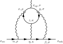
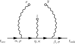
Figure 1: The connected light-by-light diagram. There are five other diagrams like the one on the left that correspond to distinct ways of connecting the photons to the muon line (or equivalently, the quark loop).

In the past, we evaluated the QED weighting function, $i^{3}\mathcal{G}_{\rho,\sigma,\kappa}(x,y,z)$, on a finite size lattice, which resulted in $1/L^{2}$ finite volume errors, where $L$ is the size of the lattice that is used to evaluate $i^{3}\mathcal{G}_{\rho,\sigma,\kappa}(x,y,z)$ Blum:2015gfa . This lattice was referred to as the QED box. Although one can make the QED box much larger than the QCD box Jin:2015bty , it is far better to compute the QED weighting function in infinite volume (and in the continuum) directly as proposed in Ref. Asmussen:2016lse ; Green:2015sra .

It may be useful to recall the finite-volume effects expected in the calculation of the hadronic light-by-light scattering contributions we are studying. The mass gap of QCD has two implications for a hadronic correlation function such as $\mathcal{H}^{C}_{\rho,\sigma,\kappa,\nu}(x,y,z,x_{\operatorname{op}})$: (1) The correlation function will decrease exponentially as the space-time distances between its arguments grow; (2) For fixed locations of its arguments, the finite-volume errors in such a correlation function will fall exponentially in the linear size of the volume in which it is computed. Therefore, if we evaluate the QED weighting function in infinite volume, which is the focus of this paper, and keep the positions $x;y;z;x_{\text{op}}$ fixed, all finite-volume errors will be exponentially suppressed as the linear lattice size grows. Since the QED weighting does not grow exponentially when the separations between $x,y,z$ increase, the summation in Eq. (5) converges exponentially implying that all finite-volume errors in the result for the muon anomaly are exponentially suppressed. For the same reason, one concludes that the finite-volume errors for the lattice calculation of the hadronic vacuum polarization (HVP) contribution to the muon $g-2$ [16] decrease exponentially as the lattice volume is increased. This conclusion will remain true when the QED corrections are included, if they are treated by a method similar to that used here. One should keep in mind that the use of an infinite-volume photon propagator in other contexts may not achieve the same reduction of finite-volume errors in the HLBL case studied here.

In this work, we demonstrate our method to compute the QED weighting function in infinite volume which differs significantly from the one proposed in Ref. Asmussen:2016lse . The paper is organized as follows: In Sec. II, we perform some analytic calculations and reduce the 12 dimensional integration in $\mathfrak{G}_{\sigma,\kappa,\rho}(y,z,x)$ to a four dimensional integration, which we then integrate numerically with the CUBA library cubature rules Hahn:2004fe . We also introduce a subtraction for $\mathfrak{G}_{\sigma,\kappa,\rho}(y,z,x)$ which does not alter the final result for $F_{2}$ in the infinite volume and continuum limits of the QCD part. In Sec. III, we show results of a pure QED light-by-light calculation carried out in a fashion similar to that of Ref. Blum:2015gfa , but using the new infinite volume QED weighting function and compare the two. In addition, we demonstrate that the new subtracted QED weighting function reduces the remaining exponentially suppressed finite volume and $\mathcal{O}(a^{2})$ discretization errors for $F_{2}$.

II Formulation

Here we show how $\mathfrak{G}_{\sigma,\kappa,\rho}(y,z,x)$ is evaluated using Eq. (I) in infinite volume. As usual, we work in Euclidean space time, and the free muon and photon propagator take the form

$$S_{{\mu}}(x,y) = \int\frac{d^{4}p}{(2\pi)^{4}}\frac{1}{i\not{p}+m}e^{ip\cdot(x-y)}=\left(-\not\hskip-1.5pt{\partial}_{x}+m\right)\int\frac{d^{4}p}{(2\pi)^{4}}\frac{1}{p^{2}+m^{2}}e^{ip\cdot(x-y)},$$ (16)

$$G(x,y) = \int\frac{d^{4}p}{(2\pi)^{4}}\frac{1}{p^{2}}e^{ip\cdot(x-y)}=\frac{1}{4\pi^{2}}\frac{1}{(x-y)^{2}}.$$ (17)

The wall- source and sink muon propagators that create and annihilate muons at rest appropriate for our kinematic setup can be evaluated as

$$\lim_{t_{\text{snk}}\rightarrow\infty}e^{m_{{\mu}}t_{\text{snk}}}\int_{\vec{x}_{\text{snk}}}S_{{\mu}}\left(x_{\text{snk}},\beta\right) = \frac{\gamma_{0}+1}{2}e^{m_{{\mu}}\beta_{t}},$$ (18)

$$\lim_{t_{\text{src}}\rightarrow-\infty}e^{-m_{{\mu}}t_{\text{src}}}\int_{\vec{x}_{\text{src}}}S_{{\mu}}\left(\alpha,x_{\text{src}}\right) = \frac{\gamma_{0}+1}{2}e^{-m_{{\mu}}\alpha_{t}}.$$ (19)

The matrix $\frac{\gamma_{0}+1}{2}$ is a projection operator, so

$$\mathfrak{G}_{\sigma,\kappa,\rho}(y,z,x) = \frac{\gamma_{0}+1}{2}\mathfrak{G}_{\sigma,\kappa,\rho}(y,z,x)\frac{\gamma_{0}+1}{2}.$$ (20)

Since $m_{{\mu}}$ is the only relevant scale in this function, without loss in generality, we set $m_{{\mu}}=1$. Starting with Eqs.  (18) and (19), we find

$$\lim_{t_{\text{snk}}\rightarrow\infty}e^{m_{{\mu}}\left(t_{\text{snk}}-\eta_{t}\right)}\int_{\beta}G(y,\beta)\int_{\vec{x}_{\text{snk}}}S_{{\mu}}\left(x_{\text{snk}},\beta\right)i\gamma_{\sigma}S_{{\mu}}(\beta,\eta) = \frac{\gamma_{0}+1}{2}i\gamma_{\sigma}\left(-\not{\hskip-2.0pt\partial_{y}}+\gamma_{0}+1\right)f(\eta-y),$$ (21)

$$\lim_{t_{\text{src}}\rightarrow-\infty}e^{-m_{{\mu}}\left(\eta_{t}-t_{\text{src}}\right)}\int_{\alpha}G(x,\alpha)\int_{\vec{x}_{\text{src}}}S_{{\mu}}(\eta,\alpha)i\gamma_{\rho}S_{{\mu}}\left(\alpha,x_{\text{src}}\right) = \left(\not{\hskip-2.0pt\partial_{x}}+\gamma_{0}+1\right)i\gamma_{\rho}\frac{\gamma_{0}+1}{2}f(x-\eta),$$ (22)

where

$$f(x)=f(|x|,x_{t}/|x|) = \frac{1}{8\pi^{2}}\int_{0}^{1}dye^{-yx_{t}}K_{0}(y|x|),$$ (23)

and $K_{0}(x)$ is a modified Bessel function of the second kind of order 0. Next, substitute Eqs. (21) and (22) into Eq. (I) to obtain

$$\mathfrak{G}_{\sigma,\kappa,\rho}(y,z,x) = \frac{\gamma_{0}+1}{2}i\gamma_{\sigma}\left(-\not{\hskip-2.0pt\partial_{y}}+\gamma_{0}+1\right)i\gamma_{\kappa}\left(\not{\hskip-2.0pt\partial_{x}}+\gamma_{0}+1\right)i\gamma_{\rho}\frac{\gamma_{0}+1}{2}$$ (24)

$$\times\frac{1}{4\pi^{2}}\int d^{4}\eta\frac{1}{(\eta-z)^{2}}f(\eta-y)f(x-\eta).$$

Before continuing to evaluate this function, let us prove some of its useful properties. It should be noted that based on the definition, Eq. (I), the function $\mathfrak{G}_{\sigma,\kappa,\rho}(y,z,x)$ has a logarithmic infrared divergence. This might raise concern about whether it is correct to evaluate only the QED part of the light-by-light amplitude in infinite volume. In fact we show below that the infrared divergence can be avoided by using a new definition of the weighting function.

Recall that $\gamma_{{\mu}}$ and $S_{{\mu}}(x,y)$ are Hermitian Dirac matrices which satisfy $\Sigma_{2}\gamma_{{\mu}}\Sigma_{2}=(\gamma_{{\mu}})^{T}$ and $\Sigma_{2}S_{{\mu}}(x,y)\Sigma_{2}=[S_{{\mu}}(x,y)]^{T}$. The free propagator is also translationally invariant, so $S_{{\mu}}(x,y)=S_{{\mu}}(-y,-x)$. As a result, one can show that

$$\Sigma_{2}\mathfrak{G}_{\sigma,\kappa,\rho}(y,z,x)\Sigma_{2} = [\mathfrak{G}_{\rho,\kappa,\sigma}(-x,-z,-y)]^{T},$$ (25)

$${}[\mathfrak{G}_{\sigma,\kappa,\rho}(y,z,x)]^{\dagger} = -\mathfrak{G}_{\rho,\kappa,\sigma}(-x,-z,-y).$$ (26)

It immediately follows that

$$\Sigma_{2}\mathfrak{G}_{\sigma,\kappa,\rho}(y,z,x)\Sigma_{2} = -[\mathfrak{G}_{\sigma,\kappa,\rho}(y,z,x)]^{\ast}.$$ (27)

Combining this result with Eq. (20), we can parameterize $\mathfrak{G}_{\sigma,\kappa,\rho}(y,z,x)$ as

$$\mathfrak{G}_{\sigma,\kappa,\rho}(y,z,x) = \frac{1+\gamma_{0}}{2}[(a_{\sigma,\kappa,\rho}(y,z,x))_{k}\Sigma_{k}+ib_{\sigma,\kappa,\rho}(y,z,x)]\frac{1+\gamma_{0}}{2},$$ (28)

where $(a_{\sigma,\kappa,\rho}(y,z,x))_{k}$ and $b_{\sigma,\kappa,\rho}(y,z,x)$ are real functions. Although the function $\mathfrak{G}_{\sigma,\kappa,\rho}(y,z,x)$ is not Hermitian, the non-Hermitian part has no projection to the magnetic moment. So, for the purpose of obtaining $F_{2}$, we only need to evaluate its Hermitian component. Because we need to symmetrize the arguments of the function in Eq. (I), we can freely permute the arguments of $\mathfrak{G}_{\sigma,\kappa,\rho}(y,z,x)$ without changing $F_{2}$. This allows us to define a new version of the function:

$$\mathfrak{G}^{(1)}_{\sigma,\kappa,\rho}(y,z,x) = \frac{1}{2}\mathfrak{G}_{\sigma,\kappa,\rho}(y,z,x)+\frac{1}{2}[\mathfrak{G}_{\rho,\kappa,\sigma}(x,z,y)]^{\dagger}$$ (29)

$$= \frac{1}{2}\mathfrak{G}_{\sigma,\kappa,\rho}(y,z,x)-\frac{1}{2}\mathfrak{G}_{\sigma,\kappa,\rho}(-y,-z,-x).$$

As a special case, when all three coordinates are the same, we immediately have

$$\mathfrak{G}^{(1)}_{\sigma,\kappa,\rho}(z,z,z) = 0,$$ (30)

since $\mathfrak{G}_{\sigma,\kappa,\rho}(y,z,x)$ only depends on relative coordinates, or distance between its arguments. Because the divergence of the function $\mathfrak{G}_{\sigma,\kappa,\rho}(y,z,x)$ is infrared and logarithmic, it is independent of the coordinates, $x$, $y$, $z$. One simple consequence of this behavior and Eq. (30) is that the new version $\mathfrak{G}^{(1)}_{\sigma,\kappa,\rho}(y,z,x)$ is infrared finite. Recall that the new version $\mathfrak{G}^{(1)}_{\sigma,\kappa,\rho}(y,z,x)$ is the same as the original $\mathfrak{G}_{\sigma,\kappa,\rho}(y,z,x)$ after substituting into Eq. (I) and projecting onto the magnetic moment. While the non-Hermitian part of the original QED weighting function has a logarithmic infrared divergence, it does not contribute to the magnetic moment.

With Eqs. (24) and (29), we obtain an infrared finite integration formula for $\mathfrak{G}^{(1)}_{\sigma,\kappa,\rho}(y,z,x)$:

$$\mathfrak{G}^{(1)}_{\sigma,\kappa,\rho}(y,z,x) = \frac{\gamma_{0}+1}{2}i\gamma_{\sigma}\left(\not{\hskip-2.0pt\partial_{\zeta}}+\gamma_{0}+1\right)i\gamma_{\kappa}\left(\not{\hskip-2.0pt\partial_{\xi}}+\gamma_{0}+1\right)i\gamma_{\rho}\frac{\gamma_{0}+1}{2}$$

$$\times\frac{1}{4\pi^{2}}\int d^{4}\eta\frac{1}{(\eta-z)^{2}}\left.\frac{f(\eta-y+\zeta)f(x-\eta+\xi)-f(y-\eta+\zeta)f(\eta-x+\xi)}{2}\right|_{\xi=\zeta=0}.$$

This four dimensional integration is performed with the CUBA library’s Cuhre routine Hahn:2004fe , which makes use of cubature rules and evaluates the integration in a deterministic way. Since performing the numerical integration is costly and the lattice calculation needs values of this function for many different values of its arguments, we pre-compute $i^{3}\mathcal{G}_{\rho,\sigma,\kappa}(x,y,z)$ for a range of points and then approximate this function by interpolating the computed values, which is similar to the strategy used in Ref. Asmussen:2016lse . The arguments of the function $i^{3}\mathcal{G}_{\rho,\sigma,\kappa}(x,y,z)$ have 12 degrees of freedom. With the help of translation and spatial rotational symmetries, the relevant number of degrees of freedom is reduced to five. These five parameters are chosen to be

$$p_{0}=(d/6)^{1/2} ,\quad d=|y-z|,$$ (32)

$$p_{1}=\alpha^{1/2} ,\quad \alpha=|x-z|/d,$$ (33)

$$p_{2}=\theta/\pi ,\quad \theta=\angle_{y-z,\hat{t}},$$ (34)

$$p_{3}=\varphi/\pi ,\quad \varphi=\angle_{x-z,\hat{t}},$$ (35)

$$p_{4}=\eta/\pi ,\quad \eta=\angle_{\overrightarrow{x-z},\overrightarrow{y-z}}.$$ (36)

Because $i^{3}\mathcal{G}_{\rho,\sigma,\kappa}(x,y,z)$ is symmetric with respect to permutation of its arguments, without loss of generality, for the purpose of interpolation, we require $|y-z|\geqslant|x-y|\geqslant|x-z|$ (this is unrelated to the restriction used for sampling the $x-y$ point pairs on the quark loop). We also limit the length $d$ to be less than $6$ (or roughly 11 fm) which should be large enough for the purpose of computing the hadronic light-by-light diagrams on our lattices. We employ a straight forward generalization of bilinear interpolation for the five dimensional interpolation (the interpolated function is linear with respect to any of its arguments within the small region between the known data points), and the grid has uniform spacing in all directions with $0\leqslant p_{i}\leqslant 1$. We have computed interpolation grids with sizes $6^{5}$, $8^{5}$, $10^{5}$, $12^{5}$, $14^{5}$, and $16^{5}$. In contrast to Ref. Asmussen:2016lse , we do not average over the muon propagation direction, so our time direction is special. Thus we have a five- instead of a three-dimensional grid. The two additional dimensions make the interpolation harder, but as we shall see, the interpolation error remains under very good control.

Although we introduced $\mathfrak{G}^{(1)}_{\sigma,\kappa,\rho}(y,z,x)$ in addition to $\mathfrak{G}_{\sigma,\kappa,\rho}(y,z,x)$, their differences will vanish immediately after projecting to the magnetic moment contribution and substituting into Eq. (I). However, due to the conservation of electric-current in the hadronic four-point correlation function, we enjoy even more freedom in choosing $\mathfrak{G}_{\sigma,\kappa,\rho}(y,z,x)$. We introduce yet another version,

$$\mathfrak{G}^{(2)}_{\sigma,\kappa,\rho}(y,z,x) = \mathfrak{G}^{(1)}_{\sigma,\kappa,\rho}(y,z,x)-\mathfrak{G}^{(1)}_{\sigma,\kappa,\rho}(z,z,x)-\mathfrak{G}^{(1)}_{\sigma,\kappa,\rho}(y,z,z).$$ (37)

With this definition, $\mathfrak{G}^{(2)}_{\sigma,\kappa,\rho}(y,z,x)$ has the property that

$$\mathfrak{G}^{(2)}_{\sigma,\kappa,\rho}(z,z,x)=\mathfrak{G}^{(2)}_{\sigma,\kappa,\rho}(y,z,z) = 0.$$ (38)

To demonstrate that these additional two terms in Eq. (37) do not contribute to the final result, recall the current conservation law for $\mathcal{H}^{C}_{\rho,\sigma,\kappa,\nu}(x,y,z,x_{\operatorname{op}})$:

$$\partial_{x_{\rho}}\left[\sum_{x_{\text{op}}}\frac{1}{2}\epsilon_{i,j,k}\left(x_{\text{op}}-x_{\operatorname{ref}}\right)_{j}i\mathcal{H}^{C}_{\rho,\sigma,\kappa,k}(x,y,z,x_{\operatorname{op}})\right] = 0.$$ (39)

Based on arguments similar to those given in Eqs. (22)-(24) of Ref. Blum:2015gfa , we conclude that

$$\sum_{x}\left[\sum_{x_{\text{op}}}\frac{1}{2}\epsilon_{i,j,k}\left(x_{\text{op}}-x_{\operatorname{ref}}\right)_{j}i\mathcal{H}^{C}_{\rho,\sigma,\kappa,k}(x,y,z,x_{\operatorname{op}})\right] = 0,$$ (40)

provided surface terms are neglected. Similar conclusions hold for the sums over $y$ and $z$ as well. This implies that

$$\sum_{x,y,z}\mathfrak{G}^{(1)}_{\sigma,\kappa,\rho}(y,z,z)\left[\sum_{x_{\text{op}}}\frac{1}{2}\epsilon_{i,j,k}\left(x_{\text{op}}-x_{\operatorname{ref}}\right)_{j}i\mathcal{H}^{C}_{\rho,\sigma,\kappa,k}(x,y,z,x_{\operatorname{op}})\right] = 0.$$ (41)

This equation demonstrates that if we substitute the subtraction terms defined in Eq. (37) back through Eqs. (I) and (11) and finally into Eq. (4), which gives their contribution to the anomalous moment, we will obtain zero. Since we use Eq. (I) to obtain the QED weighting function, the symmetry between $x$, $y$, $z$ is not affected by the definition of $\mathfrak{G}^{(2)}_{\sigma,\kappa,\rho}(y,z,x)$, and Eq. (5) can still be derived for this new function.

The neglect of surface terms in Eqs. (40) and (41) and our use of a non-conserved, local current implies that Eq. (41) strictly holds only in the infinite-volume and continuum limits. In other words, for finite volume or non-zero lattice spacing, $\mathfrak{G}^{(1)}_{\sigma,\kappa,\rho}(y,z,x)$ and $\mathfrak{G}^{(2)}_{\sigma,\kappa,\rho}(y,z,x)$ are subject to different finite volume and lattice spacing effects. Lattice fermion propagators are different from their continuum counterparts mostly in the short-distance region where the source and sink coordinates are the same, or separated by only a few lattice spacings. Hence the dominant discretization errors most likely come from this region. Since the new QED weighting function satisfies Eq. (38), it will suppress the contribution from this region along with its associated discretization error. As a result, we expect smaller discretization effects if we switch from $\mathfrak{G}^{(1)}_{\sigma,\kappa,\rho}(y,z,x)$ to $\mathfrak{G}^{(2)}_{\sigma,\kappa,\rho}(y,z,x)$. As we shall see in Sec. III, the new QED weighting function indeed generates a smaller discretization error, and fortunately, a smaller finite volume error as well.

III Results

Following Ref. Blum:2015gfa , we test this new framework by performing a pure QED light-by-light calculation where the analytic result is well known Laporta:1991zw ; Laporta:1992pa ; Kuhn:2003pu . That is, we replace the quark propagators in Eq. (13) with a leptonic loop. In Ref. Blum:2015gfa , we studied the case where the lepton loop mass was equal to the muon mass, $m=m_{{\mu}}$. In this study, we also investigate the case where the loop mass is two times the muon mass, $m=2m_{{\mu}}$. For both cases, we compare results for weighting functions $\mathfrak{G}^{(1)}_{\sigma,\kappa,\rho}(y,z,x)$ and $\mathfrak{G}^{(2)}_{\sigma,\kappa,\rho}(y,z,x)$.

We compute $F_{2}$ from Eq. (5). As mentioned before, sums over $\tilde{x}_{\text{op}}$ and $\tilde{z}$ are performed over the complete lattice volume, but the sum over $r$ is performed stochastically by sampling $x$-$y$ point pairs. In order to reduce the statistical uncertainty from this stochastic process, we sample all pairs with $r\leqslant 6$ in lattice units, up to discrete symmetries. These amount to 183 $x$-$y$ pairs. For $r>6$, we sample $r$ with the following empirically chosen distribution.

$$p(r) \propto \frac{e^{-2m|r|}}{|r|^{3}}.$$ (42)

In all the cases presented below, we sampled $4096$ pairs with $r>6$. For each pair, we compute $F_{2}$ with the corresponding pre-computed, interpolated, function $i^{3}\mathcal{G}_{\rho,\sigma,\kappa}(x,y,z)$ with grid sizes $N=6,8,10,12,14,16$. The $F_{2}$ values for different grids are strongly correlated. We extrapolate to $N\rightarrow\infty$ with a second-order fit in $1/N^{2}$, using three values with $N=8,12,16$. In Fig. 2, we plot fit curves corresponding to typical volumes and lattice spacings for the lepton loop.

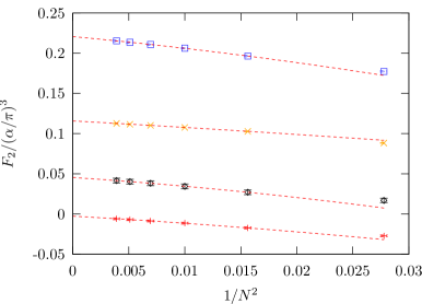
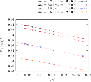
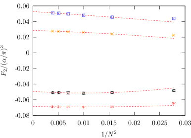
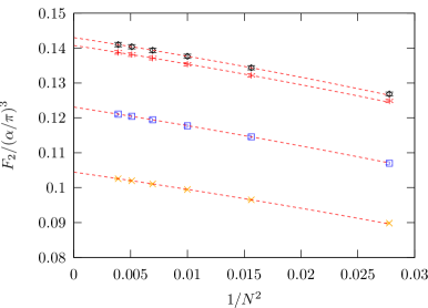
Figure 2: Extrapolations taking the number of interpolation grid points $N\to\infty$ for various lattices used in this study. The six points for each volume and lattice spacing correspond to $N=6,8,10,12,14,16$. The curves are second-order fits to $1/N^{2}$, based on the three points $N=8,12,16$. The upper two plots correspond to $m=m_{{\mu}}$, the lower two, $m=2m_{{\mu}}$. The left two plots correspond to $\mathfrak{G}^{(1)}$ and the right two plots correspond to $\mathfrak{G}^{(2)}$.

After removing the interpolation error for $i^{3}\mathcal{G}_{\rho,\sigma,\kappa}(x,y,z)$, we study non-zero lattice spacing and finite volume effects. The results are plotted in Fig. 3, and the parameter values are listed in Tab. 2. The finite volume and non-zero lattice spacing effects are much reduced by using $\mathfrak{G}^{(2)}$ instead of $\mathfrak{G}^{(1)}$, and the curves for different volumes appear to be quite parallel. Note that in the latter case some points even have the wrong sign. The difference between the $ma=0.1$ and $ma=0.2$ results is a good indicator of the non-zero lattice spacing effects. Since we have obtained results for $ma=0.1$ and $0.2$ for three volumes, this difference demonstrates the volume dependence of the non-zero lattice spacing effects. We show this comparison in Tab. 3. The $mL=4.8$ and $6.4$ points agree within errors for both loop masses. The volume $mL=3.2$ shows similar effects, but in some cases, given our high statistical precision, we observe a small difference. This is expected since the non-zero lattice spacing effects become independent of volume in the large volume limit. We also study the lattice spacing dependence of the finite volume effects in Tab. 4. It can be seen from the table that the finite volume effects are roughly independent of lattice spacing. The finite volume effects at fixed lattice spacing $ma=0.2$ are shown in Tab. 5, and we expect that the finite volume effects in the continuum limit are similar. With this table, we can see that the finite volume effect, falling exponentially with the linear size of the lattice, becomes negligible for $mL=9.6$.

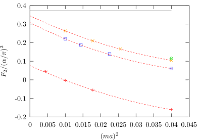
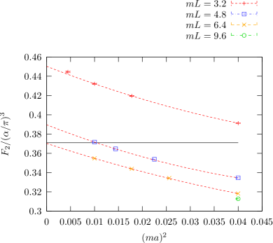
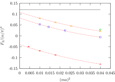
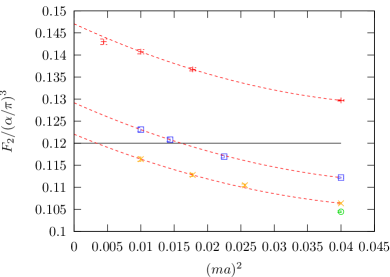
Figure 3: Leptonic light-by-light contribution to the muon anomaly, with the lepton loop mass $m=m_{{\mu}}$ (upper) and $m=2m_{{\mu}}$ (lower). The continuum, infinite volume, result is $0.371\times(\alpha/\pi)^{3}$ for $m=m_{{\mu}}$ Laporta:1991zw and $0.120\times(\alpha/\pi)^{3}$ for $m=2m_{{\mu}}$ Laporta:1992pa ; Kuhn:2003pu . The lefthand plots correspond to $\mathfrak{G}^{(1)}_{\sigma,\kappa,\rho}(y,z,x)$ and the righthand to $\mathfrak{G}^{(2)}_{\sigma,\kappa,\rho}(y,z,x)$. For each volume, we draw a second-order line which exactly passes through the three points with $ma=0.1$, 0.12 $\operatorname{or}0.133333$, and 0.2 to guide the eye. Note that the vertical scales between the plots on the left and right are different. The discretization error observed on the left is larger than on the right by a factor of four, or more, while the finite volume errors are larger by a factor of two, or more. The parameters for these curves are given in Tab. 2.

Table 2: Fits of the muon anomaly after taking the number of interpolation grid points $N\to\infty$ for non-zero lattice spacing shown Fig. 3.

$m/m_{{\mu}}$	$mL$	$F_{2}/(\alpha/\pi)^{3}$ using $\mathfrak{G}^{(1)}$	$F_{2}/(\alpha/\pi)^{3}$ using $\mathfrak{G}^{(2)}$
1	3.2	$0.0765(41)-8.58(37)(ma)^{2}+66(7)(ma)^{4}$	$0.4502(23)-1.92(22)(ma)^{2}+11.3(4.1)(ma)^{4}$
1	4.8	$0.3080(43)-9.59(44)(ma)^{2}+85(9)(ma)^{4}$	$0.3896(27)-1.94(28)(ma)^{2}+14.1(5.3)(ma)^{4}$
1	6.4	$0.3443(26)-8.83(23)(ma)^{2}+71(5)(ma)^{4}$	$0.3703(19)-1.63(18)(ma)^{2}+8.2(3.4)(ma)^{4}$
2	3.2	$-0.0407(41)-2.98(40)(ma)^{2}+19(8)(ma)^{4}$	$0.1471(18)-0.70(16)(ma)^{2}+6.6(3.0)(ma)^{4}$
2	4.8	$0.0823(39)-3.20(42)(ma)^{2}+25(8)(ma)^{4}$	$0.1292(26)-0.67(27)(ma)^{2}+6.2(5.2)(ma)^{4}$
2	6.4	$0.1083(23)-2.94(22)(ma)^{2}+19(5)(ma)^{4}$	$0.1220(17)-0.62(16)(ma)^{2}+5.8(2.9)(ma)^{4}$

Table 3: Volume dependence of non-zero lattice spacing effects in the muon anomaly. Differences between $F_{2}$ at $ma=0.1$ and $ma=0.2$ are shown for each volume.

$m/m_{{\mu}}$	$mL$	$\Delta F_{2}/(\alpha/\pi)^{3}$ using $\mathfrak{G}^{(1)}$	$\Delta F_{2}/(\alpha/\pi)^{3}$ using $\mathfrak{G}^{(2)}$
1	3.2	$0.1580(13)$	$0.0408(7)$
1	4.8	$0.1597(9)$	$0.0370(6)$
1	6.4	$0.1584(8)$	$0.0365(6)$
2	3.2	$0.0614(13)$	$0.0110(5)$
2	4.8	$0.0588(8)$	$0.0109(5)$
2	6.4	$0.0594(8)$	$0.0100(6)$

Table 4: Lattice spacing dependence of finite volume effects for the muon anomaly. Differences between $F_{2}$ with lattice size $L$ and $6.4/m$ are shown for two lattice spacings, $ma=0.1$ and $ma=0.2$.

$m/m_{{\mu}}$	$mL$	$ma$	$\Delta F_{2}/(\alpha/\pi)^{3}$ using $\mathfrak{G}^{(1)}$	$\Delta F_{2}/(\alpha/\pi)^{3}$ using $\mathfrak{G}^{(2)}$
1	3.2	0.1	$-0.2658(15)$	$0.0773(9)$
1	3.2	0.2	$-0.2654(5)$	$0.0730(4)$
1	4.8	0.1	$-0.0425(12)$	$0.0168(8)$
1	4.8	0.2	$-0.0438(4)$	$0.0163(4)$
2	3.2	0.1	$-0.1494(14)$	$0.0243(7)$
2	3.2	0.2	$-0.1514(6)$	$0.0233(3)$
2	4.8	0.1	$-0.0280(10)$	$0.0067(7)$
2	4.8	0.2	$-0.0274(5)$	$0.0058(3)$

Table 5: Volume dependence of the muon anomaly at fixed non-zero lattice spacing. $ma=0.2$. It can be seen that the infinite volume value can be approximated by the largest volume ($mL=9.6$) result. The column “diff” is the finite volume effect at this volume and lattice spacing, calculated by taking the difference between $F_{2}/(\alpha/\pi)^{3}$ given in that row and in the $mL=9.6$ row.

$m/m_{{\mu}}$	$mL$	$F_{2}/(\alpha/\pi)^{3}$ using $\mathfrak{G}^{(1)}$	diff	$F_{2}/(\alpha/\pi)^{3}$ using $\mathfrak{G}^{(2)}$	diff
1	3.2	$-0.1607(4)$	$-0.2765(5)$	$0.3913(3)$	$0.0785(4)$
1	4.8	$0.0609(3)$	$-0.0548(4)$	$0.3346(3)$	$0.0217(4)$
1	6.4	$0.1047(3)$	$-0.0110(4)$	$0.3182(3)$	$0.0054(4)$
1	9.6	$0.1157(4)$	0	$0.3128(3)$	0
2	3.2	$-0.1300(5)$	$-0.1586(6)$	$0.1297(2)$	$0.0252(3)$
2	4.8	$-0.0060(4)$	$-0.0346(5)$	$0.1122(2)$	$0.0077(3)$
2	6.4	$0.0214(4)$	$-0.0072(5)$	$0.1064(2)$	$0.0019(3)$
2	9.6	$0.0286(4)$	0	$0.1044(2)$	0

Since the finite volume effects are exponentially suppressed with lattice size $L$ and the non-zero lattice spacing effects are of order $a^{2}$, the lepton anomaly scales like

$$F_{2}(L,a) = F_{2}+\mathcal{O}(e^{-mL})+\mathcal{O}((ma)^{2}).$$ (43)

So far, from Tab. 3 and Tab. 5, we have made two observations: 1) the non-zero lattice spacing effect becomes approximately independent of volume when $mL\geqslant 4.8$; 2) the finite volume effect becomes negligible for $mL=9.6$. Based on these two observations, we fit all of the $mL\geqslant 4.8$ data with the following second-order formula:

$$F_{2}(L,a) = F_{2}(L)+k_{1}a^{2}+k_{2}a^{4}.$$ (44)

To study the systematic effects, we also fit the data with a third-order formula:

$$F_{2}(L,a) = F_{2}(L)+k_{1}a^{2}+k_{2}a^{4}+k_{3}a^{6}.$$ (45)

We do not assume any specific functional form of $F_{2}(L)$. Instead, we assume

$$F_{2} \approx F_{2}(9.6/m).$$ (46)

In this scheme, we show final results for two fermion loop masses and for $\mathfrak{G}^{(1)}$ and $\mathfrak{G}^{(2)}$ in Tab. 6. We can see that our method, with the third-order fit, has successfully reproduced the analytic calculation within our statistical precision in all cases. For $\mathfrak{G}^{(1)}$ the 2nd order fits disagree outside of statistical errors, but the values are still quite close, within five percent or less. Using 3rd order fits and $\mathfrak{G}^{(2)}$ for central values, and the difference between 2nd and 3rd order fits as a systematic error, we find

$$F_{2}/(\alpha/\pi)^{3} = 0.3686(37)(35),$$ (47)

$$F_{2}/(\alpha/\pi)^{3} = 0.1232(30)(28),$$ (48)

for $m/m_{\mu}=1$ and $2$, respectively. Here, the first error is statistical and the second systematic. These values agree within one standard deviation to the analytic results Laporta:1991zw ; Laporta:1992pa ; Kuhn:2003pu , 0.371 and 0.120, for the two loop masses.

Table 6: The muon anomaly in the continuum and infinite volume from fits to values with $mL=4.8,6.4,9.6$. Results are given for 2nd order ($F_{2}(L)+k_{1}a^{2}+k_{2}a^{4}$) and 3rd order ($F_{2}(L)+k_{1}a^{2}+k_{2}a^{4}+k_{3}a^{6}$) fits. “dof” denotes degrees of freedom, and $\chi^{2}$ is an uncorrelated chi-squared value from the fit. The analytic results are computed using continuum, infinite volume, perturbation theory Laporta:1991zw ; Laporta:1992pa ; Kuhn:2003pu .

$m/m_{{\mu}}$	order	dof	$F_{2}/(\alpha/\pi)^{3}$ using $\mathfrak{G}^{(1)}$	$\chi^{2}$	$F_{2}/(\alpha/\pi)^{3}$ using $\mathfrak{G}^{(2)}$	$\chi^{2}$
1	2	$9-5=4$	$0.3522(14)$	11.3	$0.3651(10)$	2.5
1	3	$9-6=3$	$0.3647(51)$	2.8	$0.3686(37)$	1.4
1	analytic					$0.371$
2	2	$9-5=4$	$0.1146(13)$	3.6	$0.1204(9)$	$4.5$
2	3	$9-6=3$	$0.1153(44)$	3.6	$0.1232(30)$	$3.6$
2	analytic					$0.120$

Finally, to illustrate how exponentially-suppressed finite volume errors compare with the power-law suppressed finite volume effects seen in Ref. Blum:2015gfa , we show the values from Tab. XI in Ref. Blum:2015gfa and from Tab. 2 in Fig. 4. The curves shown in the figure, which are not fits, demonstrate the expected volume dependence of the old finite volume QED weighting function and the new infinite volume one. The simple scaling curves also do not account for possible volume dependence of pre-factors. The rightmost green, plus sign point for the infinite-volume weighting function $\mathfrak{G}^{(1)}$ lies a bit off the corresponding curve. This most likely results because the discretization error has not been completely removed by the simple ansatz given in Tab. 2. This is confirmed in Tab. 6, where for $m/m_{\mu}=1$ the 2nd and 3rd order fit values for $\mathfrak{G}^{(1)}$ do not agree well. Note the 2nd order fit is especially poor. Still, we can clearly see that the curves for the infinite volume QED weighting functions approach the analytic result much faster than the curve for the finite volume QED weighting function, as expected.

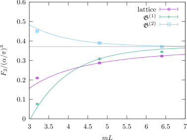
Figure 4: Volume dependence of the muon anomaly for infinite and finite volume QED weighting functions. The diamonds correspond to the finite volume QED weighting function computed on the lattice Blum:2015gfa . The plus signs and squares correspond to infinite volume QED weighting functions $\mathfrak{G}^{(1)}$ and $\mathfrak{G}^{(2)}$, respectively. Values are listed in Tab. 2. Curves correspond to expected finite volume scaling ($0.371+k/L^{2}$) and infinite volume scaling ($0.371+ke^{-mL}$), where the coefficient $k$ is chosen to match the data at $mL=4.8$. The right most point for the finite volume weighting function lies a bit off its scaling curve because the discretization error has not been completely removed by the simple ansatz given in Tab. 2, and the coefficient $k$ does not contain any possible volume dependence.

IV Conclusion

In this paper we outlined an approach to eliminate the $1/L^{2}$ finite volume errors in previous hadronic light-by-light calculations Blum:2016lnc ; Blum:2015gfa . This work was very much motivated by the recent progress made in Ref. Asmussen:2016lse . In comparison, our approach requires less analytic calculation but more numerical effort. Since we do not average over the direction of the propagating muon line, our function $i^{3}\mathcal{G}_{\rho,\sigma,\kappa}(x,y,z)$ depends on five parameters instead of three, which makes the interpolation harder. However, as we have demonstrated in Sec. III, these difficulties have been overcome. We noticed that one has freedom in choosing the QED weighting function $i^{3}\mathcal{G}_{\rho,\sigma,\kappa}(x,y,z)$ without affecting the final result. This added freedom can potentially reduce the discretization and finite volume errors. In particular, we find that the choice $\mathfrak{G}^{(2)}$ defined by Eq. (37) is much better than the original $\mathfrak{G}^{(1)}$ defined in Eqs. (29) and (I). We are now applying the new infinite volume QED weighting function $i^{3}\mathcal{G}_{\rho,\sigma,\kappa}(x,y,z)$ obtained in this work to the hadronic four-point correlation function already computed (and saved) in our previous work Blum:2016lnc .

V Acknowledgements

We thank our RBC and UKQCD collaborators for helpful discussions and support. The BAGEL Boyle:2009vp library was used to verify the code to compute free DWF propagators with fast Fourier transforms using FFTW Frigo:1999:FFT:301618.301661 . The CPS Jung:2014ata software package is also used in the calculation. In addition, we thank RBRC for BG/Q computer time. Computations were mainly performed under the ALCC Program of the US DOE on the Blue Gene/Q (BG/Q) Mira computer at the Argonne Leadership Class Facility, a DOE Office of Science Facility supported under Contract De-AC02-06CH11357. Computations were also supported through resources provided by the Scientific Data and Computing Center (SDCC) at Brookhaven National Laboratory (BNL), a DOE Office of Science User Facility supported by the Office of Science of the U.S. Department of Energy. The SDCC is a major component of the Computational Science Initiative (CSI) at BNL. L.C.J. is supported by the Department of Energy, Laboratory Directed Research and Development (LDRD) funding of BNL, under contract DE-SC0012704. T.I., C.J., and C.L. are supported in part by US DOE Contract DE-SC0012704(BNL). T.I. is supported in part by JSPS KAKENHI Grant Numbers JP26400261, JP17H02906, and also is supported by MEXT as ”Priority Issue on Post-K computer” (Elucidation of the Fundamental Laws and Evolution of the Universe) and JICFuS. T.B. is supported by US DOE grant DE-FG02-92ER40716. N.H.C. is supported in part by US DOE grant #DE-SC0011941. M.H. is supported in part by Japan Grants-in-Aid for Scientific Research, No.16K05317. C.L. acknowledges support through a DOE Office of Science Early Career Award.

References

- [1] Thomas Blum, Norman Christ, Masashi Hayakawa, Taku Izubuchi, Luchang Jin, Chulwoo Jung, and Christoph Lehner. Connected and Leading Disconnected Hadronic Light-by-Light Contribution to the Muon Anomalous Magnetic Moment with a Physical Pion Mass. Phys. Rev. Lett., 118(2):022005, 2017.
- [2] Thomas Blum, Norman Christ, Masashi Hayakawa, Taku Izubuchi, Luchang Jin, and Christoph Lehner. Lattice Calculation of Hadronic Light-by-Light Contribution to the Muon Anomalous Magnetic Moment. Phys. Rev., D93(1):014503, 2016.
- [3] Nils Asmussen, Jeremy Green, Harvey B. Meyer, and Andreas Nyffeler. Position-space approach to hadronic light-by-light scattering in the muon on the lattice. PoS, LATTICE2016:164, 2016.
- [4] Jeremy Green, Oleksii Gryniuk, Georg von Hippel, Harvey B. Meyer, and Vladimir Pascalutsa. Lattice QCD calculation of hadronic light-by-light scattering. Phys. Rev. Lett., 115(22):222003, 2015.
- [5] D. Hanneke, S. Fogwell, and G. Gabrielse. New Measurement of the Electron Magnetic Moment and the Fine Structure Constant. Phys.Rev.Lett., 100:120801, 2008.
- [6] Tatsumi Aoyama, M. Hayakawa, Toichiro Kinoshita, and Makiko Nio. Tenth-Order Electron Anomalous Magnetic Moment — Contribution of Diagrams without Closed Lepton Loops. Phys. Rev., D91(3):033006, 2015.
- [7] Michel Davier, Andreas Hoecker, Bogdan Malaescu, and Zhiqing Zhang. Reevaluation of the Hadronic Contributions to the Muon g-2 and to alpha(MZ). Eur.Phys.J., C71:1515, 2011.
- [8] Kaoru Hagiwara, Ruofan Liao, Alan D. Martin, Daisuke Nomura, and Thomas Teubner. and alpha() re-evaluated using new precise data. J.Phys., G38:085003, 2011.
- [9] J. Beringer et al. The review of particle physics. Phys. Rev., D86:010001, 2012. Including the 2013 update for the 2014 edition at http://pdg.lbl.gov.
- [10] Alexander Kurz, Tao Liu, Peter Marquard, and Matthias Steinhauser. Hadronic contribution to the muon anomalous magnetic moment to next-to-next-to-leading order. Phys. Lett., B734:144–147, 2014.
- [11] G.W. Bennett et al. Final Report of the Muon E821 Anomalous Magnetic Moment Measurement at BNL. Phys.Rev., D73:072003, 2006.
- [12] J. Grange et al. Muon (g-2) Technical Design Report. 2015.
- [13] R. M. Carey et al. The New (g-2) Experiment: A proposal to measure the muon anomalous magnetic moment to +-0.14 ppm precision. 2009.
- [14] M. Aoki et al. An Experimental Proposal on a New Measurement of the Muon Anomalous Magnetic Moment g-2 and Electric Dipole Moment at J-PARC. KEK-J-PARC, PAC2009:12, 2009.
- [15] Thomas Blum, Saumitra Chowdhury, Masashi Hayakawa, and Taku Izubuchi. Hadronic light-by-light scattering contribution to the muon anomalous magnetic moment from lattice QCD. Phys.Rev.Lett., 114(1):012001, 2015.
- [16] T. Blum. Lattice calculation of the lowest order hadronic contribution to the muon anomalous magnetic moment. Phys. Rev. Lett., 91:052001, 2003.
- [17] Luchang Jin, Thomas Blum, Norman Christ, Masashi Hayakawa, Taku Izubuchi, and Christoph Lehner. Hadronic Light by Light Contributions to the Muon Anomalous Magnetic Moment With Physical Pions. PoS, LATTICE2015:103, 2016.
- [18] T. Hahn. CUBA: A Library for multidimensional numerical integration. Comput. Phys. Commun., 168:78–95, 2005.
- [19] S. Laporta and E. Remiddi. The Analytic value of the light-light vertex graph contributions to the electron (g-2) in QED. Phys. Lett., B265:182–184, 1991.
- [20] S. Laporta and E. Remiddi. The Analytical value of the electron light-light graphs contribution to the muon (g-2) in QED. Phys. Lett., B301:440–446, 1993.
- [21] Johann H. Kuhn, A. I. Onishchenko, A. A. Pivovarov, and O. L. Veretin. Heavy mass expansion, light by light scattering and the anomalous magnetic moment of the muon. Phys. Rev., D68:033018, 2003.
- [22] Peter A. Boyle. The BAGEL assembler generation library. Comput. Phys. Commun., 180:2739–2748, 2009.
- [23] Matteo Frigo. A fast fourier transform compiler. In Proceedings of the ACM SIGPLAN 1999 Conference on Programming Language Design and Implementation, PLDI ’99, pages 169–180, New York, NY, USA, 1999. ACM.
- [24] Chulwoo Jung. Overview of Columbia Physics System. PoS, LATTICE2013:417, 2014.
- [25] The CPS software repository can be found at https://github.com/RBC-UKQCD/cps.