Precise orbital elements, masses and parallax of the spectroscopic–interferometric binary HD 26441

Abstract

The orbit of the visual–speckle binary A 2801 (HD 26441) was calculated independently of the previously published double-lined spectroscopic solution, obtaining similar values for the common orbital elements. In this way, it has been possible to provide a consistent 3D orbit and precise values for both the orbital parallax and the individual masses of the components, so the physical properties of this stellar system are determined.

1 Introduction

Double-lined spectroscopic binaries that are optically resolved with high-resolution techniques are a fundamental source of information in stellar astronomy. Indeed, once both orbits have been determined with high precision, the spectroscopic one by means of radial velocities and the visual one from the relative positions, we can obtain not only the three-dimensional orbit of the system but also the individual masses of the components as well as the orbital parallax. Such parallaxes are important because they may be used to check the values obtained by astrometric space missions, such as Gaia.

Since speckle interferometry (Labeyrie, 1970) was applied to double-star astronomy, it has created a revolution in the precision of the measurements. Moreover, several authors (McAlister, 1976, 1977, 1978; Balega & Ryadchenko, 1984; Balega et al., 1984; Bonneau et al., 1986) have used it to resolve binaries the study of which had previously been restricted to radial velocities. The combination of the two techniques yields values for parameters that are essential for the investigation of stellar evolution.

Along this line of work we present the HD 26441 (A 2801; ADS 3041; WDS 04107 $-$0452) system, the orbit of which, as a double-lined spectroscopic binary, was obtained by Griffin (Griffin, 2015) with a period of 7527 days.

Although in this case the binary had been resolved by means of micrometer measurements for nearly a century, and in 1961 with an optical interferometer by Finsen, it was only in 1996 that the first speckle observations were carried out by E. Horch. The micrometric measurements are summarized in Table 1, in which the first three columns correspond to the date, position angle (in degrees), and separation (in arcseconds). The fourth column shows the observed apparent magnitudes of both stars (C. E. Worley reported $\Delta$m = 0 in his observation of 1975.720), and the fifth, the number of observing nights. The sixth column includes the observer code, and finally, the seventh, the telescope aperture (in metres). The observer codes correspond to: B, van den Bos; VOU, Voute; VBS, Van Biesbroeck; MUL, Muller; HLN, Holden; WOR, Worley.

Table 2 lists the interferometric measurements, taken from the Fourth Catalog of Interferometric Measurements of Binary Stars (Hartkopf et al., 2001b). The first five columns include the date, the position angle and separation (with uncertainties when available). Column six shows the difference in magnitude and its uncertainty. A colon after the measurement indicates a dubious value. E. P. Horch indicated that the uncertainty of $\Delta$m is 0.12 in his observation of 2008.7024. On the other hand, the combined magnitude (7.50) is only available from Hipparcos. The seventh and eighth columns correspond to the filter used and its full-width half maximum in nanometres. The rest of the columns are the aperture of the telescope (in metres), the number of observing nights, the original reference and the code of the technique (following the format of the catalog). The reference codes are as follows: FIN61, Finsen (1961); ISO90, Isobe et al. (1990); PER97, Perryman et al. (1997); HOR01, Horch et al. (2001); HOR12, Horch et al. (2012); TOK10, Tokovinin et al. (2010); TOK12, Hartkopf et al. (2012); RID15, Riddle et al. (2015); TOK14, Tokovinin et al. (2014); TOK15, Tokovinin et al. (2015); HOR15, Horch et al. (2015); TOK16, Tokovinin et al. (2016). The techniques correspond to: J, visual interferometry; S, speckle interferometry; Hh, Hipparcos measurement; St, Tokovinin speckle camera (SOAR); Ag, laser-guided adaptive optics.

Table 1: Micrometric measurements.

Date	$\theta$	$\rho$	Mag.	n	Obs.	Tel.
	(∘)	(′′)				(m.)
1936.33	2.8	0.18	8.3–8.3	3	B	0.7
1937.68	183.1	0.20	8.0–8.0	4	VOU	0.6
1938.68	184.1	0.19		4	VOU	0.6
1941.07	21.7	0.17	8.0–8.0	1	B	0.7
1944.33	202.9	0.17	8.2–8.2	2	VBS	2.1
1944.72	216.3	0.16		4	VOU	0.6
1953.73	168.8	0.12		2	MUL	0.9
1955.01	354.7	0.14		6	VBS	2.1
1955.52	356.0	0.18	8.2–8.3	2	B	0.7
1956.17	357.7	0.19		3	MUL	0.6
1958.03	5.1	0.18	8.4–8.5	1	B	2.1
1958.09	357.3	0.20	8.4–8.6	1	B	2.1
1959.14	12.2	0.14	8.2–8.2	2	VBS	2.1
1959.967	12.1	0.19		1	VBS	1.0
1960.192	11.8	0.16		1	VBS	2.1
1961.77	15.0	0.17	8.3–8.5	4	B	0.9
1972.920	183.3	0.20		1	HLN	1.0
1975.720	348.3	0.16		3	WOR	1.5

Table 2: Interferometric measurements.

Date	$\theta$	$\sigma_{\theta}$	$\rho$	$\sigma_{\rho}$	$\Delta$m	Filter	FWHM	Tel.	n	Ref.	Tech.
	(∘)	(∘)	(′′)	(′′)		(nm.)	(nm.)	(m.)
1961.09	21.3		0.180		0.0			0.7	1	FIN61	J
1988.8030	unresolved							2.1	1	ISO90	S
1988.8057	unresolved							2.1	1	ISO90	S
1991.25	unresolved					511	222	0.3	1	PER97	Hh
1996.8984	355.5		0.169			503	40	2.1	1	HOR01	S
2008.7024	47.5	1.4	0.100	0.003	0.52	550	40	3.5	1	HOR12	S
2008.7702	47.1	0.2	0.0995	0.0003	0.8	551	22	4.1	1	TOK10	S
2010.8920	76.0	0.3	0.0685	0.0005	0.0:	788	132	4.1	2	TOK12	St
2010.8920	76.5	0.3	0.0548	0.0003	0.9	534	22	4.1	2	TOK12	St
2010.9657	75.6	0.3	0.0707	0.0002	0.9	534	22	4.1	2	TOK12	St
2012.7572	unresolved					754	119	1.5	1	RID15	Ag
2013.7369	146.4	0.3	0.0386	0.0001	0.7	534	22	4.1	2	TOK14	St
2014.0457	unresolved					788	132	4.2	1	TOK15	St
2014.0457	unresolved					534	22	4.2	2	TOK15	St
2014.7583	333.9		0.0731		0.66	692	40	4.3	1	HOR15	S
2014.7583	333.9		0.0725		0.67	880	50	4.3	1	HOR15	S
2014.8538	338.7	0.6	0.0788	0.0009	0.7	788	132	4.2	2	TOK15	St
2015.0286	337.3	0.1	0.0875	0.0002	0.6	788	132	4.2	2	TOK15	St
2015.7437	344.3	0.0	0.1199	0.0005	0.7	788	132	4.1	2	TOK16	St

Several visual orbits have been calculated for this system. The first one (Muller, 1954), with a 20-year period, was revised later by Zulević (1972) and Baize (1986) who proposed circular orbits with around 40-year periods. All three of them show very large residuals for the interferometric measurements. Tokovinin et al. (2014) recovered the short-period eccentric orbit (P = 20.42 yr, e = 0.887) but it does not fit the latest measurements, which justifies a revision.

In this article, we present a three-dimensional solution for the orbit of the system based on a new astrometric orbit with a very good fit to the micrometric measurements and remarkably to the speckle ones and which, at the same time, agrees with the spectroscopic orbit on its common elements. In this way, it has been possible to present values for the masses of the components with small uncertainties and also a value for the orbital parallax which is a perfect match to that obtained by the Hipparcos mission. At present, the possible GAIA parallax has not been published.

A study of the physical properties of HD 26441 system completes this work.

2 The new astrometric orbit

In 2014, a methodology was published (Docobo et al., 2014) that allows a determination of the orbit of a spectroscopic binary when we know the parallax and a precise astrometric measurement (i.e. speckle). That methodology also has an important application which is analyzing the coherence of the speckle measurements (and all the astrometry, in general) by means of its adaptation to the spectroscopic orbit. In that way, it is possible to improve on a previous study to find out which speckle measurements should have more weight.

Following that procedure, it turned out that the speckle observations performed in 2008.7024 (Horch), 2013.7369 (Tokovinin) and 2015.0286 (Tokovinin) are the ones which fit best. They are chosen in order to use J.A. Docobo’s analytic method (Docobo, 1985, 2012) and to generate a set of relative orbits whose corresponding apparent orbits pass through the three selected points.

Once the set of orbits is obtained, it suffices to choose that with a better rms in $\theta$ and $\rho$ (taking into account also the arithmetic means, AM, of the said coordinates) with the rest of the observations. The selected orbit, which has the best fit with those requisites is very consistent, in the elements that they have in common, with the spectroscopic orbit obtained by Griffin. The weighting scheme for the micrometer measurements is described in Docobo & Ling (2003) and, for the interferometric ones, we assign weight 5 for telescopes with an aperture of less than 1m, 10 for 1–2m-class telescopes, 15 for 2–4m, and 20 for 4m and over. The micrometer measurement of 1972.920 was not taken into account in the calculations as it shows high residuals for all the visual orbits.

The new orbital elements with their uncertainties and quality indicators (RMS and AM for $\theta$ and $\rho$) are provided in Table 3. The numbers between brackets in the RMS and AM correspond to the previous orbit by Tokovinin et al. The plot of the new (solid line) and previous (dashed line) orbits can be seen in Figure 1. The observations follow the 6th Orbit Catalog (Hartkopf et al., 2001a) convention: plusses, open circles, and filled circles represent visual observations, eyepiece interferometry, and speckle interferometry, respectively.

Two new measurements that have recently been published (Horch et al., 2017) are also in good agreement with our orbit.

Table 3: New astrometric orbit.

Element	Value $\pm$ $\sigma$
P (yr)	20.616 $\pm$ 0.015
T	2014.035 $\pm$ 0.002
e	0.843 $\pm$ 0.002
a (′′)	0.161 $\pm$ 0.002
i (∘)	66.4 $\pm$ 0.5
$\Omega$ (∘)	331.8 $\pm$ 0.5
$\omega$ (∘)	248.7 $\pm$ 0.5
RMSθ (∘)	2.315 (6.853)
RMSρ (′′)	0.011 (0.017)
AMθ (∘)	0.938 ($-$4.188)
AMρ (′′)	$-$0.001 ($-$0.011)

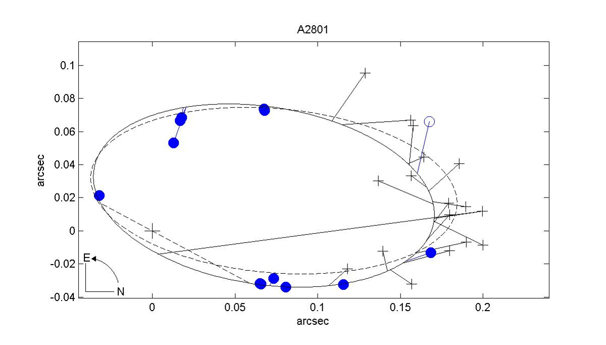
Figure 1: New (solid line) and previous (dashed line) orbit of HD 26441. Plusses represent visual observations, open circles correspond to eyepiece interferometry, and filled circles stand for speckle interferometry.

3 The spectroscopic orbit

HD 26441 was placed on the Cambridge radial-velocity observing programme by RFG in 1986; 17 observations were made on a guest-investigator basis at Haute-Provence and two at ESO, and 27 have been made in recent years with the Cambridge ‘Coravel’ spectrometer. Two periastron passages, when the ‘dips’ given by the two components were clearly separated, have been observed. A trace obtained at Cambridge, that well illustrates the unequal double-lined ‘dip’, is shown here as Fig. 2. A more comprehensive description of the radial-velocity observing campaign, and the derivation of the spectroscopic orbit with the help of 37 additional observations made by other observers with the Haute-Provence ‘Coravel’ and kindly subscribed for our use by the observers concerned, has already been published in a paper (Griffin, 2015) to which the interested reader’s attention is drawn. The orbital elements are included in Table 4, where they may be compared with the (entirely independent) astrometric elements.

Table 4: The spectroscopic orbital elements.

Element	Value $\pm$ $\sigma$
P (d)	7527 $\pm$ 4 (20.608 $\pm$ 0.011 yr)
T (MJD)	56670.5 $\pm$ 0.9 (2014.037 $\pm$ 0.003 )
$\gamma$ (km/s)	+26.55 $\pm$ 0.03
K1 (km/s)	11.59 $\pm$ 0.06
K2 (km/s)	12.51 $\pm$ 0.10
q	1.079 $\pm$ 0.010
e	0.8372 $\pm$ 0.0015
$\omega_{1}$ (∘)	69 $\pm$ 0.4
a${}_{1}\;$sin i (Gm)	656 $\pm$ 4
a${}_{2}\;$sin i (Gm)	708 $\pm$ 6
a sin i (Gm)	1364 $\pm$ 8
$\mathcal{M}_{1}$sin3i (M⊙)	0.929 $\pm$ 0.021
$\mathcal{M}_{2}$sin3i (M⊙)	0.861 $\pm$ 0.016

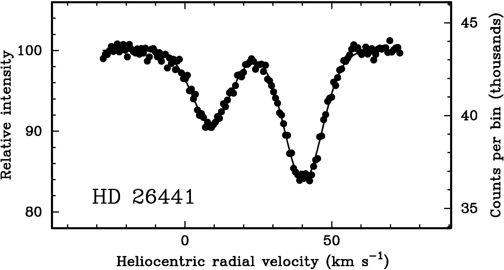
Figure 2: Radial-velocity trace of HD 26441, obtained with the Cambridge ‘Coravel’ on 2013 October 17 and showing the two dips at practically their maximum separation.

4 Parallax and masses

From the value of a sin i = 1364 $\pm$ 8 Gm (9.118 $\pm$ 0.053 astronomical units) of the spectroscopic orbit and the inclination (i = $66^{\circ}.4\pm 0^{\circ}.5$) of the visual orbit, we obtain the semimajor axis in AU:

$$a=9.950\pm 0.069AU,$$

and taking into account the value of the semi-major axis in arcseconds as given by the visual orbit, we deduce the orbital parallax of the system:

$$\pi_{orb}=\frac{a^{\prime\prime}}{a}=0^{\prime\prime}.01618\pm 0^{\prime\prime}.00023,$$ (1)

which is in perfect agreement with the Hipparcos parallax $0^{\prime\prime}.01609\pm 0^{\prime\prime}.00065$ (van Leeuwen, 2007) and which, along with the new orbital elements, gives a mass sum of 2.357 $\mathcal{M}_{\odot}$.

On the other hand, the spectroscopic orbit provides the mass ratio:

$$q=\frac{\mathcal{M}_{1}}{\mathcal{M}_{2}}=1.079\pm 0.010,$$

while the known expression, with $a$ in AU and $P$ in years:

$$\mathcal{M}_{1}+\mathcal{M}_{2}=\frac{a^{3}}{P^{2}}=2.318\pm 0.112\mathcal{M}_{\odot},$$

gives the sum of the masses. From that we deduce:

$$\begin{split}&\mathcal{M}_{1}=1.203\pm 0.059\mathcal{M}_{\odot}\\ &\mathcal{M}_{2}=1.114\pm 0.054\mathcal{M}_{\odot}.\end{split}$$ (2)

The $V$ magnitude of the star, provided by SIMBAD, is 7.37. We can estimate the difference in magnitude between the components from the speckle observations made with filters close to that band (2008.7024, 2008.7702, 2010.8920, 2010.9657, and 2013.7369) which would be 0.76. That would give us individual magnitudes, m_A = 7.81 and m_B = 8.57.

There are several measurements for the spectral types of the components but they agree in considering both components to be early–mid-G-type subgiants. For instance, Stephenson & Sanwal (1969) listed them as G3 IV–V and, independently in the same year, Christy & Walker (1969) measured a composite spectrum of G2 IV, decomposing the system in two stars of the same type, based on a $\Delta$m of $0^{\mathrm{m}}.0$. SIMBAD adopts the G3/5 IV type given in the Michigan catalogue of two-dimensional spectral types for the HD Stars, Vol. 5 (Houk & Swift, 1999).

Using those magnitudes and spectral types, and the Baize–Romani algorithm (Baize & Romani, 1946) with the parameters given in Docobo & Andrade (2013), we derive a dynamical parallax of 0${}^{\prime\prime}.$01766 for G2 IV + G4 IV spectral types, and 0${}^{\prime\prime}.$01630 for G2 V + G4 V. That is summarized in Table 5. The parallax and the mass sum of the main-sequence model are in better agreement with the values calculated in this work, and also with the Hipparcos parallax and its corresponding mass sum.

Table 5: Parallaxes and mass sums.

	Hipparcos	Orbital	Dynamical	Dynamical
			(Main seq.)	(Subgiant)
Parallax	0${}^{\prime\prime}.$01609	0${}^{\prime\prime}.$01618	0${}^{\prime\prime}.$01630	0${}^{\prime\prime}.$01766
$\sigma$	0${}^{\prime\prime}.$00065	0${}^{\prime\prime}.$00023	0${}^{\prime\prime}.$00024	0${}^{\prime\prime}.$00027
Mass	2.357 $\mathcal{M}_{\odot}$	2.318 $\mathcal{M}_{\odot}$	2.269 $\mathcal{M}_{\odot}$	1.784 $\mathcal{M}_{\odot}$
$\sigma$	0.299 $\mathcal{M}_{\odot}$	0.112 $\mathcal{M}_{\odot}$	0.011 $\mathcal{M}_{\odot}$	0.015 $\mathcal{M}_{\odot}$

5 Physical properties of the system

One of the authors of this study, RFG, has already commented (Griffin, 2015) that these stars are a bit above the main sequence. Taking into account the apparent magnitude of the system and the orbital parallax, the combined absolute magnitude (M_v) is 3.40, which is brighter than expected for a system of main-sequence stars. If we use the individual magnitudes that we obtained from $\Delta$m, we get M_v(A) = 3.84 and M_v(B) = 4.60, which are 0^m.6 and 0^m.4 brighter than the calibrated values for the main sequence (Straizys & Kuriliene, 1981) but still considerably fainter than for subgiants.

The luminosities of the components calculated from their absolute magnitudes are 2.36 and 1.17 L_⊙, respectively. Interstellar extinction was not taken into account because it is not expected to be significant at the distance of the system. For example, the Geneva–Copenhagen Survey reanalysis (GCSII, Casagrande et al. (2011)) gave a value of reddening of 0^m.032.

The effective temperatures (T_eff) derived from the spectral types are 5794 K for the primary and 5598 K for the secondary (Straizys & Kuriliene, 1981). We might find several values of the effective temperature in the literature, obtained by different methods, but all of them have the problem that they calculate the value for the whole system, not for each component separately, and this can cause a bias in the result. The GCS II gives 6031$\pm$80 K but it is included in the less-reliable clbr sample as the duplicity of the system affects the photometry. McDonald et al. (2012) used spectral-energy distributions and atmospheric models to obtain a T_eff = 5378 K for a combined luminosity of 3.89 L_⊙. The object is listed with a T_eff of 5849 K in the catalogue of Ages, Metallicities, Galactic Orbit of F stars (Marsakov & Shevelev, 1995).

The metallicity of the system, according to the GCS II, is [M/H] = 0.43, so we can use that value, along with the masses, luminosities, and T_eff to estimate the age of the system. We used the PARSEC (Bressan et al., 2012) to generate the isochrones and the evolutionary tracks with those parameters, and we find the most probable age for the system to be about 5 Gyr (see Figure 3).

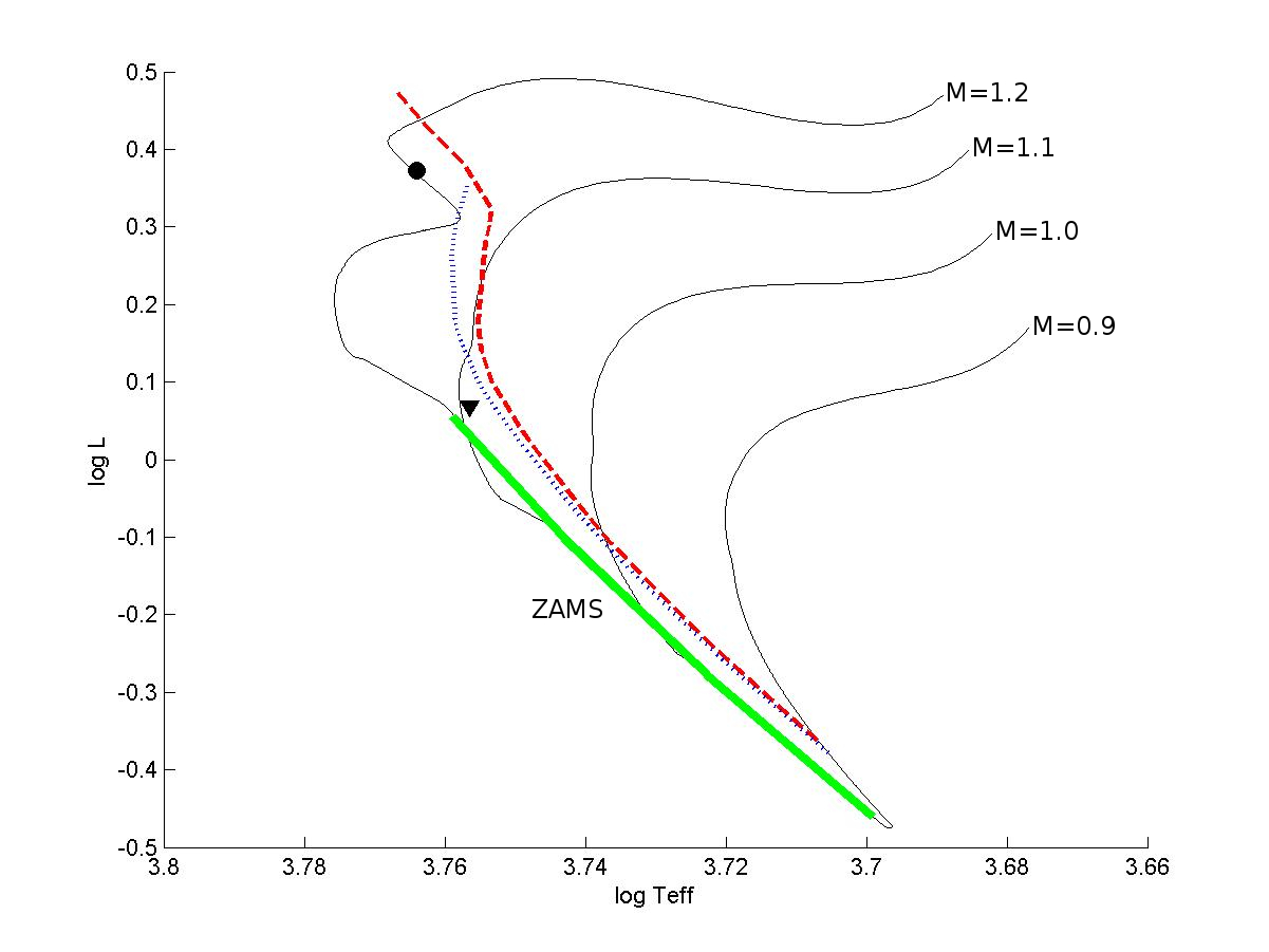
Figure 3: H–R diagram with evolutionary tracks from $\mathcal{M}$ = 0.9 $\mathcal{M}_{\odot}$ to $\mathcal{M}$ = 1.2 $\mathcal{M}_{\odot}$. The dotted line corresponds to the isochrone of 4.47 Gyr and the dashed line to the isochrone of 5.01 Gyr. The circle and the triangle represent the main and secondary components of the system, respectively. The Zero-Age Main Sequence is shown as a thick solid line.

6 Conclusions

We present a new astrometric orbit for the HD 26441 system that is in good agreement with the previous spectroscopic one by RFG in their common elements and has allowed us to calculate accurate masses and the orbital parallax of the system. We have concluded that it is comprised of two G-type stars which are beginning to evolve away from the main sequence, and we have been able to place them in their evolutionary tracks and estimate an age of about 5 Gyr for the system.

References

- Baize (1986) Baize P., 1986, A&AS, 65, 551
- Baize & Romani (1946) Baize P., Romani L., 1946, Annales d’Astrophysique, 9, 13
- Balega et al. (1984) Balega I., Bonneau D., Foy R., 1984, A&AS, 57, 31
- Balega & Ryadchenko (1984) Balega Y. Y., Ryadchenko V. P., 1984, Soviet Astronomy Letters, 10, 95
- Bonneau et al. (1986) Bonneau D., Balega Y., Blazit A., Foy R., Vakili F., Vidal J. L., 1986, A&AS, 65, 27
- Bressan et al. (2012) Bressan A., Marigo P., Girardi L., Salasnich B., Dal Cero C., Rubele S., Nanni A., 2012, MNRAS, 427, 127
- Casagrande et al. (2011) Casagrande L., Schönrich R., Asplund M., Cassisi S., Ramírez I., Meléndez J., Bensby T., Feltzing S., 2011, A&A, 530, A138
- Christy & Walker (1969) Christy J. W., Walker Jr. R. L., 1969, PASP, 81, 643
- Docobo (1985) Docobo J. A., 1985, Celestial Mechanics, 36, 143
- Docobo (2012) Docobo J. A., 2012, in Arenou F., Hestroffer D., eds, Orbital Couples: Pas de Deux in the Solar System and the Milky Way. pp 119–123
- Docobo & Andrade (2013) Docobo J. A., Andrade M., 2013, MNRAS, 428, 321
- Docobo & Ling (2003) Docobo J. A., Ling J. F., 2003, A&A, 409, 989
- Docobo et al. (2014) Docobo J. A., Campo P. P., Andrade M., Horch E. P., 2014, Astrophysical Bulletin, 69, 461
- Finsen (1961) Finsen W. S., 1961, Circular of the Union Observatory Johannesburg, 120, 367
- Griffin (2015) Griffin R. F., 2015, The Observatory, 135, 321
- Hartkopf et al. (2001a) Hartkopf W. I., Mason B. D., Worley C. E., 2001a, AJ, 122, 3472
- Hartkopf et al. (2001b) Hartkopf W. I., McAlister H. A., Mason B. D., 2001b, AJ, 122, 3480
- Hartkopf et al. (2012) Hartkopf W. I., Tokovinin A., Mason B. D., 2012, AJ, 143, 42
- Horch et al. (2001) Horch E., van Altena W. F., Girard T. M., Franz O. G., López C. E., Timothy J. G., 2001, AJ, 121, 1597
- Horch et al. (2012) Horch E. P., Bahi L. A. P., Gaulin J. R., Howell S. B., Sherry W. H., Baena Gallé R., van Altena W. F., 2012, AJ, 143, 10
- Horch et al. (2015) Horch E. P., van Belle G. T., Davidson Jr. J. W., Ciastko L. A., Everett M. E., Bjorkman K. S., 2015, AJ, 150, 151
- Horch et al. (2017) Horch E. P., et al., 2017, preprint, (arXiv:1703.06253)
- Houk & Swift (1999) Houk N., Swift C., 1999, in Michigan Spectral Survey, Ann Arbor, Dep. Astron., Univ. Michigan, Vol. 5, (1999).
- Isobe et al. (1990) Isobe S., Norimoto Y., Noguchi M., Ohtsubo J., Baba N., 1990, Publications of the National Astronomical Observatory of Japan, 1, 217
- Labeyrie (1970) Labeyrie A., 1970, A&A, 6, 85
- van Leeuwen (2007) van Leeuwen F., 2007, A&A, 474, 653
- Marsakov & Shevelev (1995) Marsakov V. A., Shevelev Y. G., 1995, Bulletin d’Information du Centre de Données Stellaires, 47, 13
- McAlister (1976) McAlister H. A., 1976, PASP, 88, 957
- McAlister (1977) McAlister H. A., 1977, ApJ, 212, 459
- McAlister (1978) McAlister H. A., 1978, ApJ, 223, 526
- McDonald et al. (2012) McDonald I., Zijlstra A. A., Boyer M. L., 2012, MNRAS, 427, 343
- Muller (1954) Muller P., 1954, AJ, 59, 388
- Perryman et al. (1997) Perryman M. A. C., et al., 1997, A&A, 323, L49
- Riddle et al. (2015) Riddle R. L., et al., 2015, ApJ, 799, 4
- Stephenson & Sanwal (1969) Stephenson C. B., Sanwal N. B., 1969, AJ, 74, 689
- Straizys & Kuriliene (1981) Straizys V., Kuriliene G., 1981, Ap&SS, 80, 353
- Tokovinin et al. (2010) Tokovinin A., Mason B. D., Hartkopf W. I., 2010, AJ, 139, 743
- Tokovinin et al. (2014) Tokovinin A., Mason B. D., Hartkopf W. I., 2014, AJ, 147, 123
- Tokovinin et al. (2015) Tokovinin A., Mason B. D., Hartkopf W. I., Mendez R. A., Horch E. P., 2015, AJ, 150, 50
- Tokovinin et al. (2016) Tokovinin A., Mason B. D., Hartkopf W. I., Mendez R. A., Horch E. P., 2016, AJ, 151, 153
- Zulević (1972) Zulević D. J., 1972, Circulaire d’Information. Commission des Étoiles Doubles, 56, 1