Magneto-optical properties of topological insulator thin films with broken inversion symmetry

Abstract

We determine the optical response of ultrathin film topological insulators in the presence of a quantizing external magnetic field taking into account both hybridization between surface states, broken inversion symmetry and explicit time reversal symmetry breaking by the magnetic field. We find that breaking of inversion symmetry in the system, which can be due to interaction with a substrate or electrical gating, results in Landau level crossings which lead to additional optical transition channels that were previously forbidden. We show that by tuning the hybridization and symmetry breaking parameters, a transition from the normal to a topological insulator phase occurs with measureable signatures in both the longitudinal and optical Hall conductivity.

LABEL:FirstPage01 LABEL:LastPage#102

I Introduction

Topological insulators fall in a class of materials known as symmetry protected topological phases. In these systems the gapless Dirac spectrum of the surface states is protected by symmetries such as charge conservation, time reversal and spatial inversion. Breaking of these symmetries leads to opening of a gap in the spectrum. In this work, we consider a subclass of these systems which are ultrathin topological insulators (TIs) with gapped Dirac cones on their top and bottom surfaces. Thin films of topological insulators have been experimentally fabricated for various TI materials such as $Sb_{2}Te_{3}$ 1a . The gap in the top and bottom surface states is usually called hybridization gap which arises as a result of coupling between top and bottom surface states of a 3D topological insulator when its thickness is sufficiently small, 5QLs (Quintuple Layers) and thinner 1b ; 1c ; 1d . This gap can be tuned by varying the thickness of topological insulator films 1e . Hence in addition to breaking of the aforementioned symmetries, gap opening in thin films is also possible through hybridization. We investigate the role of gap opening through symmetry breaking and hybridization on the optical response of the system. Specifically, we study the magneto-optical response of TI thin films with inversion symmetry breaking. Inversion symmetry breaking occurs in thin films grown on a substrate and can also be tuned by electrical gating 1c ; 1f . In both cases, chemical potential on the two surface can be different with the result that the Dirac points are not at the same energy on the two surfaces. In addition to gap tuning, another advantage of thin films is that their bulk contribution is small and allows observation of surface properties of topological insulators 1g ; 1h ; 1i . In earlier work, it was revealed that thin film topological insulators show interesting physics when time reversal symmetry is broken; either by magnetic ordering or by the application of external magnetic field 1j ; 1k ; 1l ; 1m ; 1n ; 1o . It was shown that through gap tuning, the system can make a transition from the normal insulator(NI) to a TI phase with finite dc Hall conductivity 1k ; 1m ; 1o .

The main focus of the present work is the investigation of inversion symmetry breaking effects on the magneto-optical response of TI thin films. In addition to inversion symmetry, time reversal symmetry can also be explicitly broken by a magnetic field applied to our system, which we consider. Inversion symmetry breaking generates additional gap in the spectrum of topological insulator thin films 1c . This energy gap is not only controlled by thickness of the films 1e and external exchange field/magnetic field 1j , but it can also be generated through interaction with a substrate and can be tuned by electrical gating 2a . In this paper, we show that in the presence of inversion symmetry breaking, a new feature of the Landau level spectrum is Landau level crossings which lead to new optical transition channels that can be observed in the optical response. These channels were previously forbidden in the presence of inversion symmetry. Further, we determine the dc and the optical conductivity in the quantum Hall regime and show the presence of Hall steps and plateaus even in the ac regime. We also show that by tuning the hybridization and symmetry breaking parameters, a transition from the normal to a topological insulator phase occurs with measurable signatures in the magneto-optical response.

The paper is organized as follows: In Sec. II, we present our model system. Sec. III is devoted to the calculation of the optical conductivity tensor for our system. Results for optical Hall conductivity in the quantum Hall regime are presented in Sec. IV with conclusions and summary of results in Sec. V.

II Model

Our system is a topological insulator thin film, thin enough for hybridization of surface states on the top and bottom, and broken inversion symmetry which can be either due to gating or substrate. In order to highlight the effects of Time Reversal (TR) symmetry breaking we include a term in the Hamiltonian which can arise due to magnetic ordering in the presence of magnetic dopants in the proximity of the top surface which are exchange coupled to the electronic spins. This term has been included here to illustrate the effects of TR symmetry breaking on the energy spectrum. The effective low energy Hamiltonian is 1c ; 1j ; 1f

$$H=\hbar v_{f}\tau_{z}\otimes(\sigma_{x}k_{y}-\sigma_{y}k_{x})+\Delta_{h}\tau_{x}\otimes I+\Delta_{ib}\tau_{z}\otimes I+\Delta_{z}I\otimes\sigma_{z},$$ (1)

with the basis: $|t\uparrow\rangle,|t\downarrow\rangle,|b\uparrow\rangle$ and $|b\downarrow\rangle.$ Here $t,b$ denote the top and bottom surface states and $\uparrow,\downarrow$ represent the spin up and down states. $v_{f}$ is the Fermi velocity, and $I$ is the identity matrix, $\sigma_{i}(i=x,y,z)$ and $\tau_{j}(j=x,y,z)$ are Pauli matrices acting on spin space and opposite surface space (surface pseudospin). $\Delta_{h}$ represents the hybridization between the two surface states. For large thickness $\Delta_{h}\approx 0$, hybridization of top and bottom surface states can be neglected, however when thickness is sufficiently reduced $\Delta_{h}$ generates finite gap in the Dirac spectrum. $\Delta_{ib}$ is the inversion symmetry breaking term between the two surfaces, it can result from interaction between the TI thin film and the substrate or by an electric field applied perpendicular to the surface of the thin film 1c . $\Delta_{z}$ can be the exchange field along the z-axis introduced by possible ferromagnetic ordering of the magnetic impurities. The energy spectrum of the above Hamiltonian is given by

$$\varepsilon_{\pm}^{\alpha}(k)=(-1)^{\alpha}\sqrt{\hbar^{2}v_{f}^{2}k^{2}+\Delta_{h}^{2}+\Delta_{ib}^{2}+\Delta_{z}^{2}\pm 2\sqrt{\hbar^{2}v_{f}^{2}k^{2}\Delta_{ib}^{2}+\Delta_{ib}^{2}\Delta_{z}^{2}+\Delta_{z}^{2}\Delta_{h}^{2}}},$$ (2)

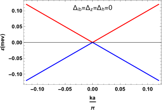
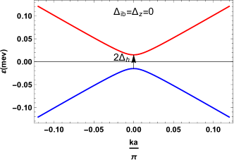
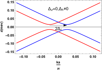
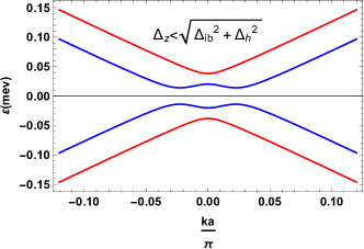
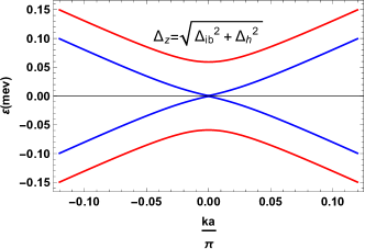
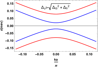
Figure 1: Schematic representation of surface band structure. (a) $\Delta_{h}=\Delta_{ib}=\Delta_{z}=0$ (b) $\Delta_{h}\neq 0,$ $\Delta_{ib}=\Delta_{z}=0$ (c) $(\Delta_{h},\Delta_{ib})\neq 0,$ $\Delta_{z}=0$ (d)$\Delta_{z}<\sqrt{\Delta_{ib}^{2}+\Delta_{h}^{2}}$ (e) $\Delta_{z}=\sqrt{\Delta_{ib}^{2}+\Delta_{h}^{2}}$ (f) $\Delta_{z}>\sqrt{\Delta_{ib}^{2}+\Delta_{h}^{2}}$

where $\alpha=1$ represents the states in valence band and $\alpha=0$ represents the states in conduction band. $\pm$  correspond to upper and lower surface. Fig. (1) shows the band structure for our system at different values of $\Delta_{h},\Delta_{ib}$ and $\Delta_{z}$. For $\Delta_{h}=\Delta_{ib}=\Delta_{z}=0$, both top and bottom surface states are gapless and degenerate. For a thin TI without any source of TR and I symmetry breaking, $(\Delta_{h}\neq 0;\Delta_{ib}=\Delta_{z}=0),$ the bands are degenerate separated by insulating gap $\Delta_{h}$. For the case of inversion asymmetry and finite hybridization with the system preserving time reversal symmetry $(\Delta_{z}=0)$, a Rashba-like splitting in the band structure occurs; Fig. 1(c). The bands are degenerate at $k=0$ as $\varepsilon_{+}^{0}(k=0)=\varepsilon_{-}^{0}(k=0)$ in conduction band and $\varepsilon_{+}^{1}(k=0)=\varepsilon_{-}^{1}(k=0)$ in valence band for all values of $\Delta_{h}$ and $\Delta_{ib}$ while for $k\neq 0$ the bands are not degenerate. This $k=0$ degeneracy is lifted by the introduction of time reversal symmetry breaking term $\Delta_{z}$, with the result that the degeneracy does not exist for any value of $k$. Therefore, the band structure represents Normal Insulator (NI) regime for small value of $\Delta_{z}$, as the value of $\Delta_{z}$ is increased the lower gap decreases. At a particular value of $\Delta_{z}$ the gap closes. This gapless point represents the phase transition point. As $\Delta_{z}$ is further increased the transition from NI to TI phase takes place and the gap reopens, (see Figs.(1e)-(1f)). The red lines (the blue lines) represent dispersion of upper (lower) surface.
Now we consider the effect of Landau quantization on the system by the application of an external magnetic field along $z$-axis directed perpendicular to the surface of TI thin film aligned in the xy-plane. The magnetic field explicitly breaks TR symmetry. In the rest of the paper we will not consider the effect of magnetic ordering. The Hamiltonian of our system takes the form 1m ; 1o ,

$$\hat{H}_{\sigma\tau}=\hbar v_{f}\tau_{z}\otimes\left[\sigma_{x}\mathbf{\pi}_{y}-\sigma_{y}\mathbf{\pi}_{x}\right]+\Delta_{h}\tau_{x}\otimes I+\Delta_{ib}\tau_{z}\otimes I+\Delta_{z}I\otimes\sigma_{z},$$

$\mathbf{\pi=k+}e\mathbf{A/}\hbar$ is the two dimensional canonical momentum with vector potential $\mathbf{A}$. Here $\Delta_{z}=g\mu_{B}B/2$ is the Zeeman energy associated with the applied magnetic field $B=B\hat{z}$, with $g$ effective Lande factor, $\mu_{B}$ is the Bohr magneton. We choose the Landau gauge for the vector potential $A=(0,xB,0).$ Since $p_{x}$ and $x$ do not commute, it is convenient to write the Hamiltonian in terms of dimensionless operators

$$\hat{H}_{\sigma\tau}=\frac{\hbar v_{f}}{\sqrt{2}l_{B}}\tau_{z}\otimes\left[\sigma_{x}l_{B}\hat{P}+\sigma_{y}\frac{\hat{Q}}{l_{B}}\right]+\Delta_{h}\tau_{x}\otimes I+\Delta_{ib}\tau_{z}\otimes I+\Delta_{z}I\otimes\sigma_{z},$$

where $l_{B}=\sqrt{c/eB}$ is the magnetic length. $\hat{Q}=-l_{B}^{2}p_{x}$ and $\hat{P}=p_{y}+\frac{eB}{\hbar}x$ such that $[\hat{Q},\hat{P}]=i\hbar$. Employing the ladder operators $a=1/\sqrt{2}l_{B}(\hat{Q}+il_{B}^{2}\hat{P})$ and $a^{\dagger}=1/\sqrt{2}l_{B}(\hat{Q}-il_{B}^{2}\hat{P}),$ we may express the Hamiltonian as:

$$H=\frac{i\hbar\omega_{B}}{\sqrt{2}}\tau_{z}\otimes(\sigma^{+}a-\sigma^{-}a^{\dagger})+\Delta_{h}\tau_{x}\otimes I+\Delta_{ib}\tau_{z}\otimes I+\Delta_{z}I\otimes\sigma_{z}$$ (3)

where $\omega_{B}=v_{F}/l_{B}$, which plays a role analogous to the cyclotron frequency in the LL spectrum of a regular 2DEG. We can write single particle eigenstates in the following form

$$\left|n\alpha s\right\rangle=u_{nT\uparrow}^{\alpha s}\left|n-1,T,\uparrow\right\rangle+u_{nT\downarrow}^{\alpha s}\left|n,T,\downarrow\right\rangle+u_{nB\uparrow}^{\alpha s}\left|n-1,B,\uparrow\right\rangle+u_{nB\downarrow}^{\alpha s}\left|n,B,\downarrow\right\rangle.$$ (4)

Here $\left|n,T(B),\uparrow(\downarrow)\right\rangle$ is the nth LL eigenstates on the top (bottom) surface with spin up (down), $\alpha=0,1$ and $s=\pm$ label the four eigenstates of Eq. (3), corresponding to each LL index $n=0,...,\infty$, and $u_{n}^{\alpha s}$ are the corresponding complex four component spinor wave functions. Thus the Hamiltonian Eq. (3) can be written in a $4\times 4$ matrix

$$H=\begin{pmatrix}\Delta_{z}+\Delta_{ib}&-i\hbar\omega_{B}\sqrt{2n}&\Delta_{h}&0\\ i\hbar\omega_{B}\sqrt{2n}&-\Delta_{z}+\Delta_{ib}&0&\Delta_{h}\\ \Delta_{h}&0&\Delta_{z}-\Delta_{ib}&i\hbar\omega_{B}\sqrt{2n}\\ 0&\Delta_{h}&-i\hbar\omega_{B}\sqrt{2n}&-(\Delta_{z}+\Delta_{ib})\end{pmatrix}.,$$ (5)

Diagonalizing the hamiltonian in Eq. (5), we find the following Landau level spectrum,

$$\epsilon_{n\alpha s}=(-1)^{\alpha}\sqrt{\Delta_{ib}^{2}+\Delta_{h}^{2}+\Delta_{z}^{2}+2n\hbar^{2}\omega_{B}^{2}+2s\sqrt{\Delta_{ib}^{2}\Delta_{z}^{2}+\Delta_{h}^{2}\Delta_{z}^{2}+2n\Delta_{ib}^{2}\hbar^{2}\omega_{B}^{2}}}.$$ (6)

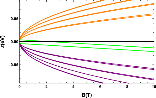
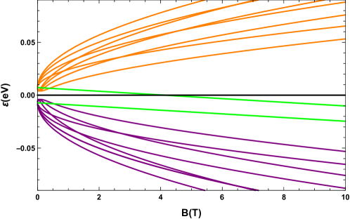
Figure 2: Landau level energies as a function of magnetic field (B) in units of  Tesla with hybridization energy $\Delta_{h}=0.004eV$, and Zeeman energy $\Delta_{z}=0.0017BeVT^{-1}.$ a: $\Delta_{ib}=0$, b: $\Delta_{ib}=0.006eV$. The $n=0$ landau levels are represented by green lines, shifting from an electron-like and hole like set to both being hole-like as the magnetic field is increased. In 2(b) the crossing of LLs can be clearly seen as a result of finite $\Delta_{ib}$

The Landau level energy spectrum is shown in Fig. (2). An important feature of the spectrum is that its electron-hole symmetric for $n\neq 0.$ The LL spectrum consists of two sets: $(i)\epsilon_{n0s}$ and $(ii)\epsilon_{n1s}$ where $\epsilon_{n1s}$ represents spectrum for occupied states below $\mu=0$ and $\epsilon_{n0s}$ represent the unoccupied states above $\mu=0$. For both sets of occupied and unoccupied Landau levels each Landau level splits in a doublet for $s=\pm 1$. This splitting results from time reversal symmetry breaking term $(\Delta_{z}),$ broken inversion symmetry and the hybridization $(\Delta_{h})$ in the Hamiltonian. There are two situations where splitting can vanish, if $(i)$ the system has inversion symmetry $(\Delta_{ib}=0)$ and broken TR symmetry along with no hybridization $(\Delta_{h}=0)$ $(ii)$ system has both TR symmetry$(\Delta_{z}=0)$ and inversion symmetry$(\Delta_{ib}=0)$ with no constraint on the hybridization (for zero hybridization with both TR and inversion symmetry thin film TI will behave like gapless Dirac material with only one $n=0$ partially filled LL at $\mu=0$). Note that the $n=0$ LL, only splits when either $\Delta_{h}$ or $\Delta_{ib}$ is nonzero. A novel feature of LLs in the presence of broken inversion symmetry is their crossings within each set, between $nth$ and $(n+1)th$ levels with opposite $s$ values, at certain values of magnetic field. There is no crossing of $n=0$ LL in our system at any value of magnetic field. We consider terms linear in $k$. However, for large values of $k$ hybridization terms must be redefined as $\frac{\Delta}{2}-Bk^{2}$. This results in crossing of the $n=0$ Landau levels. This crossing becomes an anti-crossing in the presence of inversion symmetry breaking 2b

The $n=0$ LLs behaves differently compared to $n\neq 0$ LLs. For $n=0$ Eq. (4) shows that the electrons are fully spin-polarized in these levels; only spin down levels are occupied. Hence $n=0$ levels are split into two sublevels with spin down unlike other levels which are split into four sublevels, two with spin up and two with spin down. The corresponding $n=0$ wavefunctions (un-normalized) are

$$u_{0}^{\alpha s}=\{0,s(-1)^{\alpha}\frac{(-\Delta_{ib}+s\sqrt{\Delta_{ib}^{2}+\Delta_{h}^{2}})}{\Delta_{h}},0,1\}.$$

The corresponding LL energies are

$$\epsilon_{0\alpha s}=(-1)^{\alpha}\left|\Delta_{z}+s\sqrt{\Delta_{ib}^{2}+\Delta_{h}^{2}}\right|.$$

Explicitly

$$u_{0}^{0-1} =\{0,\frac{\Delta_{ib}+\sqrt{\Delta_{ib}^{2}+\Delta_{h}^{2}}}{\Delta_{h}},0,1\},$$ (7)

$$u_{0}^{11} =\{0,\frac{\Delta_{ib}-\sqrt{\Delta_{ib}^{2}+\Delta_{h}^{2}}}{\Delta_{h}},0,1\},$$

for $\Delta_{z}<\sqrt{\Delta_{ib}^{2}+\Delta_{h}^{2}}.$

$$\epsilon_{00-1}=\left|\Delta_{z}-\sqrt{\Delta_{ib}^{2}+\Delta_{h}^{2}}\right|,\text{ \ \ \ \ \ }\epsilon_{011}=-\left|\Delta_{z}+\sqrt{\Delta_{ib}^{2}+\Delta_{h}^{2}}\right|.$$ (8)

For $\Delta_{z}>\sqrt{\Delta_{ib}^{2}+\Delta_{h}^{2}},$ $u_{0}^{0-1}$ is replaced by $u_{0}^{1-1}:$

$$u_{0}^{1-1}=\{0,\frac{\Delta_{ib}+\sqrt{\Delta_{ib}^{2}+\Delta_{h}^{2}}}{\Delta_{h}},0,1\},$$

with energy given by

$$\epsilon_{01-1}=-\left|\Delta_{z}-\sqrt{\Delta_{ib}^{2}+\Delta_{h}^{2}}\right|.$$

In the NI phase the states are $u_{0}^{0-1}$ and $u_{0}^{11}$, and in TI phase the states are $u_{0}^{1-1}$ and $u_{0}^{11}.$ Thus one of the $n=0$ electron-like sublevel becomes a hole-like sublevel which can be seen in Fig. (3) for density of states and in the Landau level spectrum in Fig. (2). This change in character of the zeroth LL manifests particle-hole symmetry breaking in the system which results in jump in Hall conductivity from $0$ to a finite value at chemical potential $\mu=0$. This signals a transition from the NI phase to the TI phase.

II.1 Density of states

The Green function associated with our Hamiltonian is

$$G(\omega,n,\alpha,s)={\displaystyle\sum\limits_{\alpha,s}}\frac{1}{\omega-(-1)^{\alpha}\sqrt{\Delta_{ib}^{2}+\Delta_{h}^{2}+\Delta_{z}^{2}+2n\hbar^{2}\omega_{B}^{2}+2s\sqrt{\Delta_{ib}^{2}\Delta_{z}^{2}+\Delta_{h}^{2}\Delta_{z}^{2}+2n\Delta_{ib}^{2}\hbar^{2}\omega_{B}^{2}}}+i\eta}.$$

From which we can compute density of states as

$$D(\omega) =\frac{-1}{2\pi l_{B}^{2}}{\displaystyle\sum\limits_{n}}ImG(\omega,n,\alpha,s),$$

$$D(\omega) =\frac{-1}{\pi}\frac{1}{2\pi l_{B}^{2}}({\displaystyle\sum\limits_{n\neq 0}}ImG(\omega,n,\alpha,s)+ImG(\omega,0,\alpha,s)).$$

The plots for density of states are shown in Fig. (3). $(NI)$ represents the normal insulator phase in which the LL spectrum has perfect particle-hole symmetry. At $\Delta_{z}>\sqrt{\Delta_{ib}^{2}+\Delta_{h}^{2}},$ both $n=0$ levels are filled as they shift to the valence band, thus breaking particle-hole symmetry for LL spectrum across $\epsilon=0$. This shift in the Landau level is associated with transition from (NI) phase to the TI phase. We notice two interesting features of the density of states: (i) At certain values of $\omega$ two adjacent peaks are closely spaced such that they tend to merge in a single peak. (ii) Some peaks have higher weight than all other peaks. These two distinct features are attributed to crossing (or near crossing) of two Landau levels at certain values of magnetic field, see Fig. (2). The parameters chosen in these plots are $\Delta_{ib}=0.006eV$, $\Delta_{h}=0.004eV$ and $\hbar v_{f}^{2}eB=1.6\times 10^{-4}B$.

III Magneto-optical conductivity

To determine the magneto-optical conductivity tensor we need eigenfunctions of the Hamiltonian given in Eq. (5). The explicit form of the eigenfunctions $u_{n}^{\alpha s}$ in Eq. (4) is

$$u_{n}^{\alpha s} =(u_{nT\uparrow}^{\alpha s},u_{nT\downarrow}^{\alpha s},u_{nB\uparrow}^{\alpha s},u_{nB\downarrow}^{\alpha s}),$$ (9)

$$u_{nT\uparrow}^{\alpha s} =\dfrac{-i}{d_{1}N}(N_{1}+sN_{2}(\Delta_{ib}+\Delta_{z})+\epsilon_{n\alpha s}(\Delta_{ib}\Delta_{z}+sN_{2})),$$ (10)

$$u_{nT\downarrow}^{\alpha s} =\dfrac{1}{d_{2}N}(\Delta_{ib}^{2}+sN_{2}+\epsilon_{n\alpha s}\Delta_{ib}),$$ (11)

$$u_{nB\uparrow}^{\alpha s} =\dfrac{-1}{d_{3}N}(N_{3}-\Delta_{h}(-\Delta_{ib}-\Delta_{z}-\epsilon_{n\alpha s})(\Delta_{ib}-\Delta_{z}-\epsilon_{n\alpha s})),$$ (12)

$$u_{nB\downarrow}^{\alpha s} =\dfrac{1}{N}.$$ (13)

$N_{1}$,$N_{2}$,$N_{3}$,$d_{1}$,$d_{2}$,$d_{3}$ are given by

$$d_{1} =\sqrt{2n}\Delta{{}_{h}}\omega{{}_{B}}(\Delta_{ib}-\Delta_{z})$$ (14)

$$d_{2} =\Delta{{}_{h}}(\Delta_{ib}-\Delta_{z})$$ (15)

$$d_{3} =2i\sqrt{2n}\Delta_{h}\omega_{B}(\Delta_{ib}-\Delta_{z})$$ (16)

$$N_{1} =\Delta_{ib}^{2}\Delta_{z}+\Delta_{h}^{2}\Delta_{z}+\Delta_{ib}\Delta_{z}^{2}+2n\omega_{B}^{2}\Delta_{ib}$$ (17)

$$N_{2} =\sqrt{\Delta_{ib}^{2}\Delta_{z}^{2}+\Delta_{h}^{2}\Delta_{z}^{2}+2n\omega_{B}^{2}\Delta_{ib}^{2}}$$ (18)

$$N_{3} =\Delta_{h}(\Delta_{h}^{2}+2n\omega_{B}^{2}),$$ (19)

and $N$ is the normalization constant. Given the above eigenfunctions we can now evaluate the magneto-optical conductivity tensor within linear response regime using Kubo formula 2c .

$$\sigma_{\alpha\beta}(\omega)=\dfrac{i\hbar}{2\pi l_{B}^{2}}\underset{n\alpha s\neq n^{\prime}\alpha^{\prime}s^{{}^{\prime}}}{\sum}\dfrac{f(\varepsilon_{n\alpha s})-f(\varepsilon_{n^{\prime}\alpha^{\prime}s^{\prime}})}{\epsilon_{n^{\prime}\alpha^{\prime}s^{\prime}}-\epsilon_{n\alpha s}}\dfrac{\left\langle n\alpha s\right|\hat{\jmath}_{\alpha}\left|n^{\prime}\alpha^{\prime}s^{\prime}\right\rangle\left\langle n^{\prime}\alpha^{\prime}s^{\prime}\right|\hat{\jmath}_{\beta}\left|n\alpha s\right\rangle}{\hbar\omega-\epsilon_{n^{\prime}\alpha^{\prime}s^{\prime}}+\epsilon_{n\alpha s}+i\hbar/(2\tau)}$$ (20)

where $\hat{\jmath}_{\alpha}=\frac{e}{\hbar}\dfrac{\partial H}{\partial k_{\alpha}}$ and $f(\varepsilon_{n\alpha s})=\frac{1}{1+exp[\beta(\epsilon_{n\alpha s}-\mu)]}$ is the Fermi distribution function with $\beta=1/k_{B}T$ and $\mu$ is the chemical potential. We note that transitions between occupied Landau levels are Pauli blocked. So the only allowed transitions will be from the occupied LLs in valence band to unoccupied LLs in conduction band (i.e. across chemical potential $\mu=0$). After evaluating the matrix elements we have found that the selection rules for allowed transitions is $n^{\prime}=n\pm 1$. The absorptive part of the conductivity for $n=0$ Landau level above and below $\mu=0$ is

$$\binom{\operatorname{Re}\sigma_{xx}(\omega)/\sigma_{0}}{Im\sigma_{xy}(\omega)/\sigma_{0}} =\hbar ev_{f}^{2}B\underset{s}{[\sum}\dfrac{(f(\epsilon_{11s})-f(\epsilon_{00-1}))N(1,0,s,1,1)\times\eta}{(\epsilon_{00-1}-\epsilon_{11s})((\hbar\omega+\epsilon_{11s}-\epsilon_{00-1})^{2}+\eta^{2})}$$

$$\pm\underset{s}{\sum}\dfrac{(f(\epsilon_{011})-f(\epsilon_{10s}))M(0,0,-1,1,s)\times\eta}{(\epsilon_{10s}-\epsilon_{011})((\hbar\omega+\epsilon_{011}-\epsilon_{10s})^{2}+\eta^{2})}$$

$$\pm \underset{n=2,ss^{\prime}\alpha\neq\alpha^{\prime}}{\sum}\dfrac{(f(\epsilon_{n\alpha s})-f(\epsilon_{n+1\alpha^{\prime}s^{\prime}}))M(n,s,s^{{}^{\prime}}\alpha,\alpha^{\prime})\times\eta}{(\epsilon_{n+1\alpha^{\prime}s^{\prime}}-\epsilon_{n\alpha s})((\hbar\omega+\epsilon_{n\alpha s}-\epsilon_{n+1\alpha^{\prime}s^{\prime}})^{2}+\eta^{2})}$$

$$+\underset{n=2,s,s^{\prime}\alpha\neq\alpha^{\prime}}{\sum}\dfrac{(f(\epsilon_{n\alpha s})-f(\epsilon_{n-1\alpha^{\prime}s^{\prime}}))N(n,s,s^{\prime},\alpha,\alpha^{\prime})\times\eta}{(\epsilon_{n-1\alpha^{\prime}s^{\prime}}-\epsilon_{n\alpha s})((\hbar\omega+\epsilon_{n\alpha s}-\epsilon_{n-1\alpha^{\prime}s^{\prime}})^{2}+\eta^{2})}],$$ (21)

and for the case when both $n=0$ LLs are hole-like Landau levels, the conductivity is

$$\binom{\operatorname{Re}\sigma_{xx}(\omega)/\sigma_{0}}{Im\sigma_{xy}(\omega)/\sigma_{0}} =\hbar ev_{f}^{2}B\underset{s}{[\sum}\dfrac{(f(\epsilon_{01-1})-f(\epsilon_{10s}))N(1,0,s,1,1)\times\eta}{(\epsilon_{10s}-\epsilon_{01-1})((\hbar\omega+\epsilon_{01-1}-\epsilon_{10s})^{2}+\eta^{2})}$$

$$\pm\underset{s}{\sum}\dfrac{(f(\epsilon_{011})-f(\epsilon_{10s}))M(0,1,-1,0,s)\times\eta}{(\epsilon_{10s}-\epsilon_{011})((\hbar\omega+\epsilon_{011}-\epsilon_{10s})^{2}+\eta^{2})}$$

$$\pm \underset{n=1,\alpha s\neq\alpha^{\prime}s^{{}^{\prime}}}{\sum}\dfrac{(f(\epsilon_{n\alpha s})-f(\epsilon_{n+1\alpha^{\prime}s^{\prime}}))M(n,\alpha,s,\alpha^{\prime},s^{{}^{\prime}})\times\eta}{(\epsilon_{n+1\alpha^{\prime}s^{\prime}}-\epsilon_{n\alpha s})((\hbar\omega+\epsilon_{n\alpha s}-\epsilon_{n+1\alpha^{\prime}s^{\prime}})^{2}+\eta^{2})}$$

$$+\underset{n=2,s,s^{\prime}\alpha\neq\alpha^{\prime}}{\sum}\dfrac{(f(\epsilon_{n\alpha s})-f(\epsilon_{n-1\alpha^{\prime}s^{\prime}}))N(n,\alpha,s,\alpha^{\prime},s^{{}^{\prime}})\times\eta}{(\epsilon_{n-1\alpha^{\prime}s^{\prime}}-\epsilon_{n\alpha s})((\hbar\omega+\epsilon_{n\alpha s}-\epsilon_{n-1\alpha^{\prime}s^{\prime}})^{2}+\eta^{2})}].$$ (22)

Here $\sigma_{0}=e^{2}/h,$ $\eta=\hbar/2\tau$ is the scattering rate related to broadening of the Landau levels and

$$M(n,\alpha,s,\alpha^{\prime},s^{{}^{\prime}})=[(u_{nT\downarrow}^{\alpha s})^{\ast}u_{n+1T\uparrow}^{\alpha^{\prime}s^{\prime}}-(u_{nB\downarrow}^{\alpha s})^{\ast}u_{n+1B\uparrow}^{\alpha^{\prime}s^{\prime}}]\times[u_{nT\downarrow}^{\alpha s}(u_{n+1T\uparrow}^{\alpha^{\prime}s^{\prime}})^{\ast}-u_{nB\downarrow}^{\alpha s}(u_{n+1B\uparrow}^{\alpha^{\prime}s^{\prime}})^{\ast}],$$ (23)

and

$$N(n,\alpha,s,\alpha^{\prime},s^{{}^{\prime}})=[(u_{nB\uparrow}^{\alpha s})^{\ast}u_{n-1B\downarrow}^{\alpha^{\prime}s^{\prime}}-(u_{nT\uparrow}^{\alpha s})^{\ast}u_{n-1T\downarrow}^{\alpha^{\prime}s^{\prime}}]\times[u_{nB\uparrow}^{\alpha s}(u_{n-1B\uparrow}^{\alpha^{\prime}s^{\prime}})^{\ast}-u_{nT\uparrow}^{\alpha s}(u_{n-1T\downarrow}^{\alpha^{\prime}s^{\prime}})^{\ast}].$$ (24)

Where $\ast$ denotes complex conjugation. First let us consider the conductivity at zero temperature. The features of the spectrum to bear in mind are: All $n\neq 0$ levels are split in a doublet $(s=\pm)$ for finite value of Zeeman energy and hybridization. The inversion symmetry breaking term $\Delta_{ib}$ results in crossing of Landau levels at different values of magnetic field strength. Therefore there are not only the allowed transitions between LLs with same $s$ but transitions can also occur between LLs with different $s.$ These transitions are not allowed in the presence of inversion symmetry1o . Hence inversion symmetry breaking opens optical transition channels which were previously forbidden.

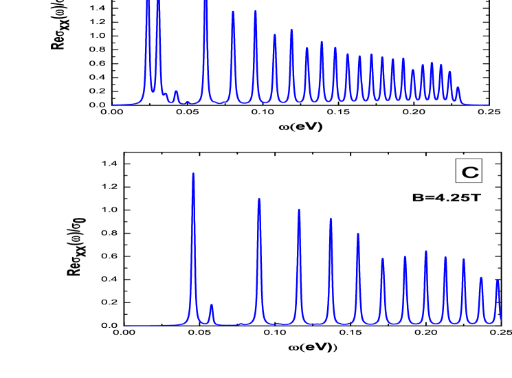
Figure 4: Real part of the longitudinal conductivity $\sigma_{xx}(\omega)$ of thin film topological insulator in units of $e^{2}/\hbar$ as a function of $\omega$ in $eV$. (a,b) normal insulator phase, (c) at CNP and (d) quantum Hall phase. All these absorption peaks are resulted from the transition across $\mu=0$.

Fig. (4) shows results for absorptive peaks from Eq. (21) and Eq. (22). All the absorptive peaks result from the transitions between LLs across $\mu=0$. In Fig. (4(a,b)), in the NI phase, the first peak corresponds to transition from $n=0$ and $n=1$ Landau level with $\omega=\epsilon_{00-1}-\epsilon_{11-1}.$ This is a single transition peak and is close to the 2nd absorption peak between the LL, $\omega=\epsilon_{10-1}-\epsilon_{011}$. Next two peaks are small and are also contributed by the Landau level transition between $n=0$ and $n=1$. The set of transitions involving $n=0$ and $n=1$ in NI phase are $\epsilon_{11s}\rightarrow\epsilon_{00-1}$ and $\epsilon_{011}\rightarrow\epsilon_{10s}$. As the magnetic field is increased which increases Zeeman energy such that at $\Delta_{z}=\sqrt{\Delta_{ib}^{2}+\Delta_{h}^{2}}$ , the LL $\epsilon_{00-1}$ becomes partially filled. At this stage one of the peaks corresponding to $n=0$ and $n=1$ transition disappears involving $n=0$ are $\epsilon_{011}\rightarrow\epsilon_{10s}$. Increasing Zeeman energy further by increasing the magnetic field such that it is greater then $4.25T$ the $n=0$ doublet becomes hole like doublet and LL $\epsilon_{00-1}$ changes to $\epsilon_{01-1}$. The allowed transitions for $n=0$ are $\epsilon_{011}\rightarrow\epsilon_{10s}$ and $\epsilon_{01-1}\rightarrow\epsilon_{10s}$ represented by peaks at $\omega=\epsilon_{10s}-\epsilon_{01-1}$ and $\omega=\epsilon_{10s}-\epsilon_{011}$. The transitions $\epsilon_{11s}\rightarrow\epsilon_{00-1}$ in NI is replaced by $\epsilon_{01-1}\rightarrow\epsilon_{10s}$ in the TI phase. The absorption peaks for $n\neq 0$ shift to higher energy in TI phase because at high magnetic field the gap between LL increases.

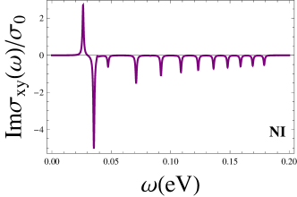
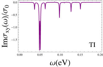
Figure 5: Imaginary part of the transverse conductivity $\sigma_{xy}(\omega)$of thin film topological insulator in units of $e^{2}/\hbar$ as a function of  $\omega$ in $eV$. a: Normal phase, b: QH phase

To understand the behavior of $Im\sigma_{xy}$ we must keep in mind the minus sign between the two terms in Eqs. (21), (22). The first two peaks result from transition between $n=0$ and $n=1$ levels, one having positive amplitude and the other having negative amplitude. The transition peaks involving $n\neq 0$ transitions have decreased in height which is due to the negative sign. For example, the transitions from $n=2$ to $n=1$ Landau level and $n=1$ to $n=2$ have same denominator and the mismatch between numerators of the two transitions results in a net negative amplitude. Fig. (5a) shows the imaginary part transverse conductivity for absorption peaks due to photon absorption in the NI phase and Fig. (5b) shows the imaginary part transverse conductivity in the TI phase.

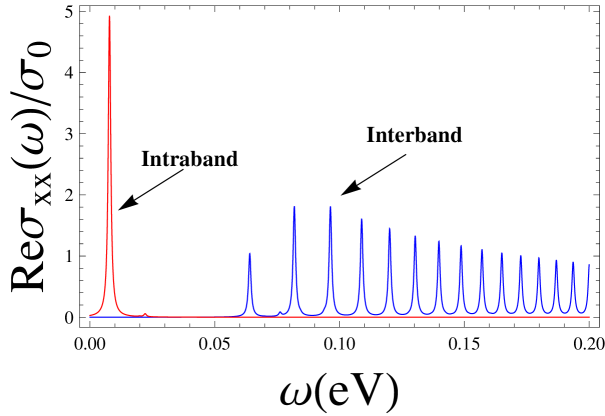
Figure 6: Real part of the longitudinal conductivity $\sigma_{xx}(\omega)$ of thin film topological insulator in units of e${}^{2}/\hbar$ as a function of $\omega$ in $eV$ for $B=2$T. Red peak represents absorption peak for intraband transition while blue peaks represent absorption peaks for interband transitions.

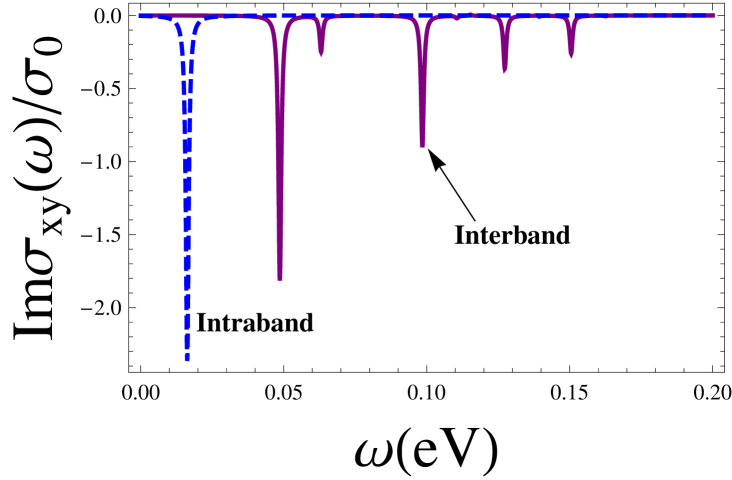
Figure 7: Imaginary part of the transverse conductivity $\sigma_{xy}(\omega)$of thin film topological insulator in units of $e^{2}/\hbar$ as a function of $\omega$ in $eV$ for $B=5$T. Blue dotted peak represents absorption peak for intraband transition while purple peaks represent absorption peaks for interband transitions.

The behavior of absorption peaks at finite chemical potential is shown in Fig. (6) and Fig. (7). For finite value of $\mu$ in the conduction band, in addition to filled LLs in valence band there are also filled LLs in conduction band resulting in allowed transition within same band(intraband transitions). Here interband and intraband transitions are defined with respect to the position of the chemical potential. These intraband absorption peaks shift to lower energy and do not split. The allowed transition within same bands (intraband transitions) have greater probability as compared to interband transitions.

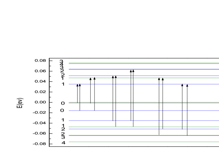
Figure 9: Schematic representation of the allowed transitions between Landau levels in quantum Hall phase at $B=5$T.

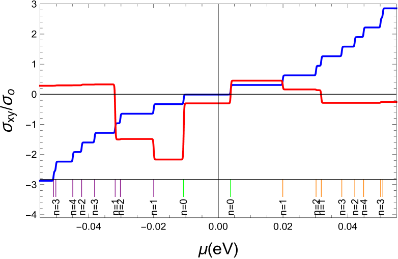
Figure 10: Static Hall conductivity(blue) and optical Hall conductivity(red) as a function of chemical potential at magnetic field $B=2$T. For optical Hall conductivity $w=0.02eV.$

Fig. (9) and Fig. (10) illustrate the allowed transitions between LLs at different values of magnetic field. The blue lines are for $s=-1$ LLs and green lines are for $s=1$ LLs. Except for $n=0$ all the other Landau levels have perfect particle-hole symmetry. The chemical potential is represented by thick black line. The vertical arrows show the allowed inter band transitions. The shift of chemical potential from $\mu=0$ to some finite value results in additional intraband transitions.

IV Optical Hall Conductivity

To calculate Hall conductivity we use wavefunctions from Eq. (4) in the Kubo formula given in Eq. (20) and obtain

$$\sigma_{\alpha\beta}(\omega) =\hbar ev_{f}^{2}B\underset{n\alpha s\neq n^{\prime}\alpha^{\prime}s^{{}^{\prime}}}{\sum}\dfrac{(f(\varepsilon_{n\alpha s})-f(\varepsilon_{n+1\alpha^{\prime}s^{\prime}}))}{(\epsilon_{n+1\alpha^{\prime}s^{\prime}}-\epsilon_{n\alpha s})}M(n,\alpha,s,\alpha^{\prime},s^{{}^{\prime}})$$ (25)

$$[\dfrac{1}{\hbar\omega-\epsilon_{n\alpha s}+\epsilon_{n+1\alpha^{\prime}s^{\prime}}+i\hbar/(2\tau)}-\dfrac{1}{\hbar\omega-\epsilon_{n+1\alpha^{\prime}s^{\prime}}+\epsilon_{n\alpha s}+i\hbar/(2\tau)}]$$ (26)

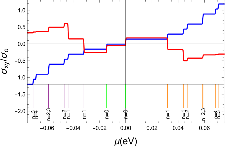
Figure 11: Static Hall conductivity(blue) and optical Hall conductivity(red) as a function of chemical potential at magnetic field $B=4.25$T. For optical Hall conductivity $w=0.02eV.$

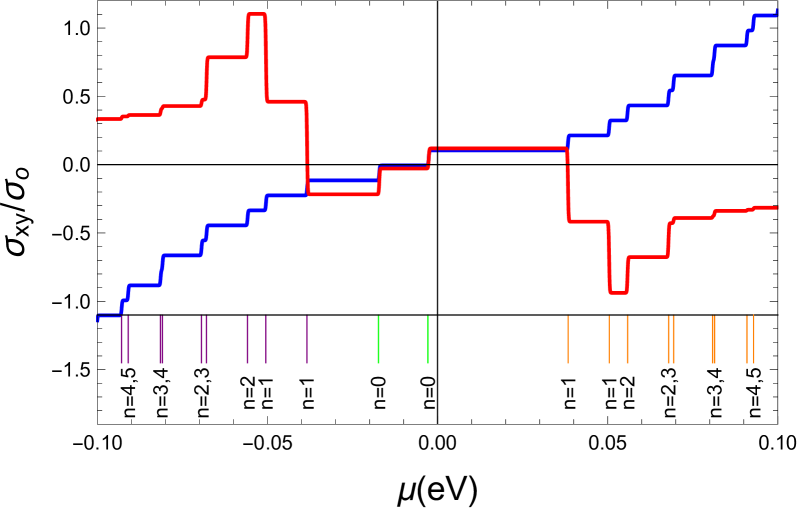
Figure 12: Static Hall conductivity(blue) and optical Hall conductivity(red) as a function of chemical potential at magnetic field $B=5.8$T. For optical Hall conductivity $w=0.02eV.$

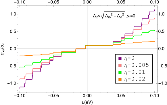
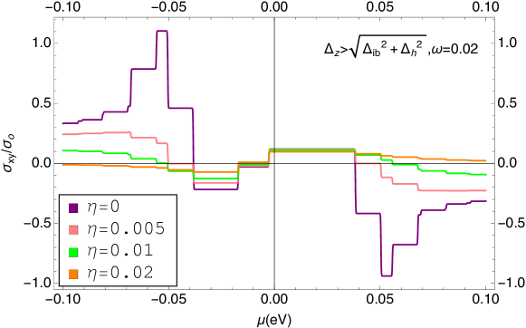
Figure 13: (a)Dc Hall conductivity for different values of $\eta$ in Quantum Hall phaase; $\Delta_{z}>\sqrt{\Delta_{ib}^{2}+\Delta_{h}^{2}}$. The structure associated with $n=0$ LLs remains while the steps for large $|n|$ diminish as $\eta$ is increased. (b) For optical Hall conductivity the $n=0$ LLs remains robust while for large $|n|$ the step-like structure diminishes more rapidly with increasing $\eta$ as compared to static case. Here $\omega$ is set at $0.02eV.$

The effects of broken inversion symmetry that are reflected in the LL spectrum and crossing of LLs are also revealed in the dc and optical Hall conductivity, which we now discuss. In Figs. (11,12,13) plots with blue color show the results for dc Hall conductivity ($\sigma_{xy}(\omega=0)$) with $B=2$T (perfect particle hole symmetry across $\mu=0$), $B=4.27$T (one $n=0$ LL is partially filled at $\mu=0$) and $B=5.8$T (one extra filled LL for negative value of $\mu$) at temperature 1K respectively. The results are presented as a function of the chemical potential $\mu$. The LL spectrum is also shown to emphasize the unusual behavior of steps and plateaus at specific magnetic fields. These steps and plateaus show clear deviation from previous results, 1n , which were in the presence of inversion symmetry. For $n\geq 1$ the plateau widths and step heights are symmetrical for both negative and positive values of $\mu,$ reflecting particle-hole symmetry in the system. However, widths and heights are not symmetrical within the same band because of LL crossings. The contribution of $n=0$ LLs to Hall conductivity pleateus shows interesting behavior. For chemical potential fixed at $\mu=0,$ the conductivity jumps from $0$ for $\Delta_{z}<\sqrt{\Delta_{ib}^{2}+\Delta_{h}^{2}}$ to a finite value for $\Delta_{z}>\sqrt{\Delta_{ib}^{2}+\Delta_{h}^{2}}$. This is an indication of phase transition from NI phase to TI phase as the magnetic field is increased. For $\Delta_{z}<\sqrt{\Delta_{ib}^{2}+\Delta_{h}^{2}}$ the $n=0$ doublet has one electron like ($u_{0}^{0-1}$) LL and one hole like ($u_{0}^{11}$). When magnetic field is increased such that $\Delta_{z}>\sqrt{\Delta_{ib}^{2}+\Delta_{h}^{2}}$ both $n=0$ LLs become hole like, thus increasing the Hall conductivity. For $n=0$ LLs the Hall conductivity jump depends on magnetic field according to $[sgn(\Delta_{z}-\sqrt{\Delta_{ib}^{2}+\Delta_{h}^{2}})+1]$. In Figs. (10,11,12) red plots represent optical Hall conductivity. The steps and plateaus are robust for low values of $n=(0,1)$ but as the value of $n$ increases, they no longer remain robust especially for $n>\pm 2.$ We note that as the value of magnetic field is increased the number of robust steps also increases, which is expected. The steps structure is symmetric across $\mu=0$ except for steps involving $n=0$ LLs. The steps corresponding to low value of $n$ are however robust unless frequency $\omega$ is close to a resonance. In the case of static hall conductivity these steps are always robust.

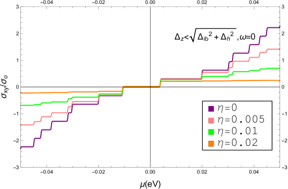
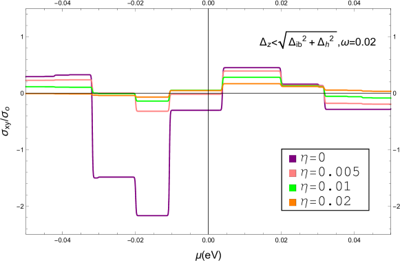
Figure 14: (a)Dc Hall conductivity for different values of $\eta$ in NI phaase; $\Delta_{z}<\sqrt{\Delta_{ib}^{2}+\Delta_{h}^{2}}$. The structure associated with $n=0$ LLs remains while the steps for large $|n|$ diminish as $\eta$ is increased. (b) For optical Hall conductivity the $n=0$ LLs remains robust while for large $|n|$ the step-like structure diminishes more rapidly with increasing $\eta$ as compared to static case. Here $\omega$ is set at $0.02eV.$

Next we examine the robustness of step-like structure in the optical Hall conductivity as function of disorder strength in both the phases of the system. The degree of disorder can be characterized by the scattering rate parameter $\eta$ 2d We present the results of our calculation for TI phase in Fig. (13). We can see that for dc hall conductivity the step-like structure remains for fairly large values of $\eta$. The step like structure for large $|n|$ begin to dminish when $\eta$ is increased. However the step corresponding to $n=0$ LLs always remains rebust. For ac Hall conductivity the step-like structure is less robust against increase in $\eta$. For $\eta\simeq\omega$ the plateaus are nearly washed out for large $|n|$, while the $n=0$ is again robust. For the case of NI phase a similar behavior is observed ; see Fig. (14).

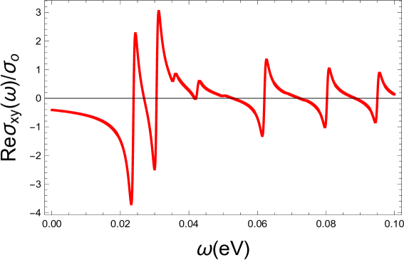
Figure 15: Optical Hall conductivity with $(\Delta_{z}<\sqrt{\Delta_{ib}^{2}+\Delta_{h}^{2}})$ for chemical potential $\mu=0.$

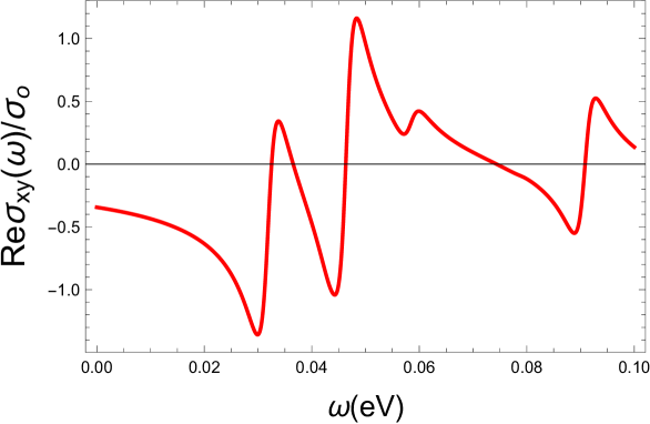
Figure 16: Optical Hall conductivity with $(\Delta_{z}>\sqrt{\Delta_{ib}^{2}+\Delta_{h}^{2}})$ for chemical potential $\mu=0$ $(i.e.$optical Hall conductivity in quantum Hall phase).

In Fig. (15) and Fig. (16) we show real part of $\sigma_{xy}(\omega)$ as a function of $\omega,$ we find that real part of $\sigma_{xy}(\omega)$ exhibits sharp cyclotron resonance peaks at transition energies for transition involving $n=0$ LL. These resonance peaks change sign near each allowed transition frequency. As for experimental realization, since the Faraday rotation angle is directly proportional to optical Hall conductivity, it is possible to observe the steps in optical Hall conductivity that are predicted here by performing Faraday rotation measurements 2d ; 2e ; 2f .

V Conclusions

To conclude, we have determined the LL spectrum, density of states and the magneto-optical conductivity tensor with in linear response regime for thin film topological insulators with finite hybridization between the surface states. We find that breaking of time reversal and inversion symmetry can have profound effects on the optical response. We have shown that inversion symmetry breaking, in addition to time reversal symmetry breaking and hybridization, significantly affects the spectrum, transition channels and magneto-optical response of the system. In the inversion symmetry broken TI thin films, we have found the following: The system can exist in Normal Insulating (NI) and Topological Insulating (TI) phases. The phase transition between these phases can be controlled by the degree of hybridization as well as by breaking symmetries: time reversal/inversion symmetry or both. The LL spectrum exhibits level crossings which were not present in the inversion symmetric system. New optical transition channels have been found which were previously forbidden. We show that there are observable signatures of the phase transition from NI to TI phase in both the longitudinal and optical Hall conductivity.

VI Acknowledgement

Kashif Sabeeh would like to acknowledge the support of the Higher Education Commission (HEC) of Pakistan through project No. 20-1484/R&D/09 and the Abdus Salam International Center for Theoretical Physics (ICTP) for support through the Associateship Scheme.

Figure 3: Density of states for thin film topological insulator in a magnetic field in units of $eB/h$. Upper (NI) Density of states in normal insulator phase $(\Delta_{z}<\sqrt{\Delta_{ib}^{2}+\Delta_{h}^{2}})$ . Lower Density of states in quantum Hall phase phase$(\Delta_{z}>\sqrt{\Delta_{ib}^{2}+\Delta_{h}^{2}})$.

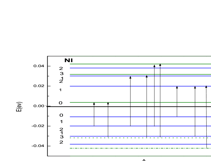
Figure 8: Schematic representation of the allowed transitions between Landau levels in normal insulator phase at $B=2$T.

References

• (1) T. Zhang, J. Ha, N. Levy, Y. Kuk, and J. Stroscio, Phys. Rev Lett. 111, 056803 (2013).
• (2) J. Linder, T. Yokoyama and A. Sudbo Phys. Rev. B 80 205401 (2009).
• (3) Y. Zhang, K. He, C.-Z. Chang, C.-L. Song, L.-L. Wang, X. Chen, J.-F. Jia, Z. Fang, X. Dai, W.-Y. Shanet al., Nat. Phys.6, 584 (2010).
• (4) H.-Z. Lu, W.-Y. Shan, W. Yao, Q. Niu, and S.-Q. Shen,Phys. Rev. B 81,115407 (2010).
• (5) C.-X. Liu, H. Zhang, B. Yan, X.-L. Qi, T. Frauenheim, X. Dai, Z. Fang, and S.-C. Zhang, Phys. Rev. B 81, 041307 (2010).
• (6) W.-Y. Shan, H.-Z. Lu, and S.-Q. Shen, New J. Phys. 12, 043048 (2010).
• (7) C.-Z. Chang, J. Zhang, X. Feng, J. Shen, Z. Zhang, M. Guo, K. Li, Y. Ou, P. Wei, L.-L. Wanget al., Science 340,167 (2013).
• (8) Hai-Zhou Lu, An Zhao, and Shun-Qing Shen Phys. Rev. Lett. 111, 146802 (2013).
• (9) Jing Wang, Biao Lian, Haijun Zhang, and Shou-Cheng Zhang Phys. Rev. Lett. 111, 086803 (2013).
• (10) R. Yu, W. Zhang, H-J. Zhang, S-C. Zhang, X. Dai and Z. Fang Science 329 61(2010).
• (11) M. Lasia and L. Brey Phys. Rev. B 90 075417 (2014).
• (12) A. A. Zyuzin, M. D. Hook, and A. A. Burkov, Phys. Rev. B 83, 245428 (2011).
• (13) A. A. Zyuzin and A. A. Burkov, Phys. Rev. B 83, 195413 (2011).
• (14) M. Tahir, K. Sabeeh, and U. Schwingenschlögl J. Appl. Phys. 113, 043720 (2013).
• (15) A. Ullah and K. Sabeeh. J. Phys. Condens. Matter 26 505303 (2014).
• (16) J. Wang, H. Mabuchi and X-L. Qi Phys. Rev.B 88 195127 (2013).
• (17) Zhang, S.B. et al. Sci. Rep. .5, 13277.
• (18) X.-L. Qi, T. L. Hughes, and S.-C. Zhang, Phys. Rev. B, 78, 195424 (2008).
• (19) Takahiro Morimoto, Yasuhiro Hatsugai, and Hideo Aoki, Phys. Rev. Lett. 103, 116803 (2009).
• (20) I. Crassee, J. Levallois, A. L. Walter, M. Ostler, A. Bostwick, E. Rotenberg, T. Seyller, D. van der Mareland, and A. B. Kuzmenko,Nat. Phys.7, 48 (2011).
• (21) R. Shimano, G. Yumoto, J. Y. Yoo, R. Matsunaga, S. Tanabe, H. Hibino, T. Morimotoand, and H. Aoki, Nat. Commun. 4, 1841 (2013).
Refer to caption
Refer to caption
Refer to caption
Refer to caption
Refer to caption
Refer to caption