Estimating the Counterparty Risk Exposure by using the Brownian motion local time

Abstract

In recent years, the counterparty credit risk measure, namely the default risk in Over The Counter (OTC) derivatives contracts, has received great attention by banking regulators, specifically within the frameworks of Basel II and Basel III. More explicitly, to obtain the related risk figures, one has first obliged to compute intermediate output functionals related to the Mark-to-Market (MtM) position at a given time $t\in[0,T]$, $T$ being a positive, and finite, time horizon. The latter implies an enormous amount of computational effort is needed, with related highly time consuming procedures to be carried out, turning out into significant costs. To overcome latter issue, we propose a smart exploitation of the properties of the (local) time spent by the Brownian motion close to a given value.

Keywords: Counterparty Credit Risk, Exposure at Default, Local times Brownian motion, Over the Counter Derivatives, Basel Financial Framework

1 Introduction

For some years now, due to the occurrence of events leading to the financial crisis between 2007 and 2008, regulators have forced financial institutions to adopt ad-hoc procedures to predict, and therefore prevent, defaults. In other words, banks have to be able to measure and manage their default risk. As concerns both the credit and the counterparty risk, in 2006 the Basel Committee for Banking Supervision has inserted in the well known Basel II reform, two rather general methodologies for calculating banks capital requirements, namely: the Standardized approach and the Internal approach. While the former one is based on the use of ratings from External Credit Rating Agencies,the latter envisages the evaluation of certain risk parameters, such as the Exposure at Default (EAD), [4].

An interesting perspective concerns the so-called Counterparty Credit Risk, (CCR), which represents the default risk linked to Over The counter (OTC) derivatives contracts. The latter case implies the computation, as intermediate outputs, of a large set of different functionals related to the Mark-to-Market, ($MtM$) of the position over a future time horizon, at a given time $t\in[0,T]$, where $T<+\infty$ is the time horizon. Standard techniques for the evaluation of such an exposure are based on classical Monte Carlo methods, which are characterized by a strong dependence on the number of considered assets and related high computational time costs, see, e.g., [38].

Other approaches have been also given, as an example the considering geometric point of view, see [45], or general ambit stochastic processes as in [21], or some optimal investment control problems, as in [17], even if, as a general benchmark, the Monte Carlo set of methods are the widest used. Nevertheless, as mentioned, Monte Carlo techniques are far from being computationally satisfactory, even in simple cases. For example, a medium bank requires $D=O(10^{4})$ derivative deals and $U=O(10^{3})$ risk factors, evaluated in $K=20$ time steps with $N=2000$ simulations, which allow for $K\cdot N\cdot U=4\cdot 10^{7}$ grid points for the risk factor simulation and $K\cdot N\cdot D=4\cdot 10^{8}$ tasks for deals evaluation.

To overcome latter drawbacks, the literature has recently proposed new techniques, e.g., the Vector Quantization [8, 12, 13, 14], or more enhanced hardware technologies, such in the case of grid computing and Graphics Processing Units (GPUs) capabilities, see, e.g., [16],[41] and references therein. In the context of American option pricing, other methods recently investigated are the martingale-based approach à la Rogers, see e.g. [34], and the simple least-squares approach, see [1],[26] for further details. A different solution can be achieved exploiting the so called polynomial chaos expansion approach, see, e.g., [6], [20] and references therein.

Another possibility consists in exploiting the properties of suitable mathematical tools, as for the case of derivatives pricing via Brownian local time. Given a probability space $(\Omega,\mathfrak{F},\mathbb{P}),$ we consider a standard Brownian Motion  $\{W_{t}\}_{t\geq 0}$ defined on it. Then, for $\omega\,\in\,\Omega$ and a level $a,$ an interesting point is to determine how much time the sample path $W_{t}(\omega)$ spends close to $a$. A possible answer dates back to the works written by Paul Lévy in 1948, where the author introduced the concept of Brownian Local Time, see [37].

The right approach consists in defining the Brownian Local Time, BLT from now on, as the following density:

$$L_{t}(a):=\frac{1}{2\epsilon}\lim_{\epsilon\longrightarrow 0}\mu\{x:|x-a|\leq\epsilon\}\;,$$ (1)

where $\mu$ represents the Lebesgue measure on the real line.

Remark 1.1.

It is worth to mention that there does not exist a standard notation to define the BLT, since some authors prefer to multiply the limit in Eq.  (1) by $\frac{1}{4\epsilon},$ instead of by $\frac{1}{2\epsilon},$ see, e.g., [32].

More formally, the local time  can be defined through the so-called occupation formula, see [32], namely by the following equation

$$\int_{0}^{t}f(W_{s})\mathrm{d}s=2\int_{\mathbb{R}}f(x)L_{t}(x)\mathrm{d}x\;,$$ (2)

where the left-hand side is a random measure, called occupation measure or sojourn measure, at fixed time $t$ and level $x\,\in\,\mathbb{R}$, while $f$ is a $L^{1}$ function, $f:\,\mathbb{R}\,\rightarrow\,\mathbb{R}.$ We refer to Section  3.2 for a more detailed discussion of the BLT properties. To what concerns the fine properties of the local time, e.g., the identification of both its distribution function and related density function and moments, we refer to [23], [32], [46], and references therein. It is also worth to mention that there exists an extended literature dealing with the theoretical applications of BLT such as an extension of Itô’s formula to convex functions, the definition of the density of the occupation measure for a Brownian Motion  with respect to the Lebesgue measure, see e.g. [8], etc.

On the other hand, a relatively limited literature has been devoted to concrete applications of BLT and its properties. The latter lack can be easily recognized in frameworks related to Economy and Finance. Nevertheless theoretical aspects of the BLT can be fruitfully exploited to analyze a wide range of financial tools, particularly with respect to the pricing of some kinds of exotic path-dependent options as in the case, e.g., of range accrual options and accumulators, where the payoff depends on the time spent by the underlying below or above a given level, resp. between two boundaries, resp. outside of them, see e.g. [39]. Moreover, the use of BLT is almost absent in the risk management field. The present work aims at filling latter gap by showing that the numerical integration of the BLT density function can be used to evaluate the risk exposure, hence obtaining results that are very compelling when compared with classical Monte Carlo benchmark algorithms.

The paper is organized as follows: in Section  2 we introduce the financial framework, focusing on the regulatory viewpoint, and with emphasis to the instructions for calculating the EAD and the Credit Value Adjustment (CVA), then, in Section  3, the mathematical setting is introduced also recalling the main properties of the BLT while, in section  4, we provide the local time approach to the aforementioned type of financial problems, also analyzing its performances compared to more standard techniques with respect to an EAD application; eventually, in Section  5, we state our main conclusions and we outline future line of research.

2 Counterparty Risk: the Financial Framework

2.1 The Credit Counterparty Risk in the Basel approach

In the Basel II framework, the Counterparty Credit Risk, CCR from now on, is a specific class of the broader credit risk category. Let us recall the definition of the Basel committee, shortly BCBS, as it is written in [4]:

Definition 2.1.

Counterparty Credit Risk (CCR) is the risk that the counterparty in a transaction could default before the final settlement of the transaction’s cash flows. An economic loss would occur if the transactions or portfolio of transactions with the counterparty has a positive economic value at the time of default.

Unlike a firm’s exposure to credit risk through a loan, CCR creates a bilateral risk of loss: the market value of the transaction is uncertain, it can be positive or negative to either counterparty and can vary over time with the movement of underlying market factors. A typical example is given by IRS. Several classes of financial transactions are considered in the regulatory perimeter, but most of the CCR arise from Over the Counter (OTC) derivatives, in the peer-to-peer relationships with a defaultable counterparty. From a practical perspective, the buyer of any option, or the holder of a derivative with positive $MtM$, both are facing a CCR. If the two counterparties agree upon a netting set,, e.g. a running compensation process in their deals, the current exposure will be given by the positive part of the algebraic sum of all deals.

As in the whole Basel setting, the risk must be dealt with by setting apart an amount regulatory capital of the bank which is linked to the risk measure called capital requirement, let us indicate it by $K$, and specified in [5], as follows

$$K =EAD\cdot 1.06\cdot LGD\left\{\Phi\left[\left(\frac{1}{1-\rho}\right)^{0.5}\Phi^{-1}(PD)+\left(\frac{\rho}{1-\rho}\right)^{0.5}\Phi^{-1}(0.999)\right]-PD\right\}\cdot c\;,$$ (3)

where:

• $EAD$ is the Exposure at Default, namely an estimation of the extent to which a bank may be exposed to a counterparty in case of default;

• $LGD$ is the Loss Given Default, namely an estimation of the percentage of the credit not recoverable in case of insolvency;

• $PD$ is the Probability of Default, namely an estimate of the likelihood that a default will occur;

• $\rho$ is the asset return correlation coefficient;

• $c$ is a constant which takes into account some maturity adjustment and can vary with respect to different regulatory portfolios, such as enterprise or retail loans;

• $1.06$ is a coefficient depending on the calibration procedure made by the Basel committee;

• $\Phi$ is the cumulative distribution function of a standard Gaussian random variable;

• $\Phi^{-1}$ is simply the inverse of $\Phi$, also referred to as the quantile function.

As well highlighted in the BCBS definition, see Def. (2.1), the EAD estimation makes the counterparty risk very different from the normal credit risk for loans and mortgages. In fact, the Basel formula  (3) requires a $1$ year measurement process, and the default time $\tau$ could be, or it could not to be, in any future time $t.$

For a mortgage, we know the future exposure profile, since it can be computed using the amortizing plan. Differently, in the CCR, the EAD estimation is fairly difficult, because of two different reasons: the future exposure is stochastic and, further, it depends on the market parameters via its specific evolution pricing model.

In other words, the CCR depends both on the credit parameters $(PD,LGD)$ and on the market influenced $EAD$ parameter in its magnitude, that is why it is also referred as the boundary risk. To summarize, the CCR has to be determined according to eq.  (3) for the credit risk, but its $EAD$ input estimation is itself a hard challenge, to which the Basel committee and the financial operators pay most of their attention.

2.2 Exposure and CVA calculation in the Basel II-III setting

In order to calculate the $EAD$ quantity in the CCR context by a robust and conservative way, the Basel II framework [4] defines two important different approaches: the Standard model and the Internal model, also called EPE-based approach.

In the standard model, we have $EAD=MtM+\mbox{\emph{Add-On}},$ where the Add-On is computed exploiting a table which depends on both the underlying asset class and on the time to maturity. In this case, the idea is that such an Add-On takes into account the future volatility by additive coefficients. As an example, for an equity option with maturity $M$ years and such that $1\leq M\leq 5$, we have that the Add-On is $8\%$ of the notional amount, while for an interest rate derivative it is just $0.5\%.$ In the EPE-based approach, to which the present work refers, some notation has to be pointed out.

• Given a derivative maturity time $0<T<+\infty$, we consider $K\in\mathbb{N}^{+}$ time steps $0<t_{1}<t_{2}<\cdots<t_{K},$ which constitute the so called buckets array, denoted by ${\bf B}^{T,K}$, where usually, but not mandatory, $t_{K}=T.$

• For every $t_{k}\in{\bf B}^{T,K}$, we denote by $MtM\left(t_{k},S_{k}\right):=MtM\left(t_{k},S_{t_{k}}\right)$ the fair value, Mark-to-Market, of a derivative at time bucket $t_{k},$ with respect to the underlying value $S_{k}$ considered at time $t_{k}$.

• For every $t_{k}\in{\bf B}^{T,K}$, we denote by $MtM\left(t_{k},S^{k}\right):=MtM\left(t_{k},S^{t_{k}}\right)$ the fair value (Mark-to-Market) of a derivative at time bucket $t_{k}$, with respect to the whole sample path $S^{k}:=\left\{S_{t}:0\leq t\leq t_{k}\right\},$ and with initial time $t_{0}=0.$

• Taking into account previous definitions, we indicate by $\varphi=\varphi\left(T-t_{k},S_{k},\Theta\right)$ the pricing function for the given derivative, where $\Theta$ represents the set of parameters from which such a pricing function may depend, e.g., the free risk rate $r$ or the volatility $\sigma.$

We give an account of the main amounts, as they are defined in Basel III [4], that will be used later on to estimate the EAD.

We denote the Expected Exposure of the derivative at time $t_{k}\,\in\,{\bf B}^{T,K}$ $(EE_{k})$, as follows

$$EE_{k}:=\frac{1}{N}\sum_{n=1}^{N}MtM\left(t_{k},S_{k,n}\right)^{+},\;N\,\in\,\mathbb{N}^{+}\;,$$ (4)

which is the arithmetic mean of the positive part of the $N$ Monte Carlo simulated MtM values, computed at the $k-$th time bucket $t_{k},$ with respect to the underlying $\mathrm{S}.$

Remark 2.2.

The positive part operator is effective if we are managing a symmetric derivative, such as an interest rate swap or a portfolio of derivatives. Nevertheless it is redundant if we consider a single option, as the fair value of the option is always positive from the buy side situation. We want to stress that the sell side does not imply counterparty risk, hence it is out of context.

We evaluate the Expected Positive Exposure (EPE) as follows

$$EPE:=\frac{1}{T}\sum_{k=1}^{K}EE_{k}\cdot\Delta_{k},$$ (5)

where $\Delta_{k}=t_{k}-t_{k-1}$ indicates the time space between two consecutive time buckets at the $k$-th level. If the time buckets $t_{k}$ are equally spaced, then the formula reduces to $EPE=\frac{1}{K}{\sum_{k=1}^{K}EE_{k}}$. Therefore, the EPE value gives the time average of the $EE_{k}$ and reflects the hypothesis that the default could happen, as a first approximation, at any time with the same probability.

We define the Effected Expected Exposure as follows

$$EEE_{1}:=EE_{1};\mbox{ and }EEE_{k}:=\max\left\{EE_{k},EEE_{k-1}\right\},\,k=1,\ldots,K\;,$$

observing that, due to its non decreasing property, $EEE_{k}$ takes into account the fact that, once the time decay effect reduces the MtM as well as the counterparty risk exposure, the bank applies a roll out with some new deals.

We also define the Effected Expected Positive Exposure (EEPE) by

$$EEPE:=\frac{1}{T}\sum_{k=1}^{K}EEE_{k}\cdot\Delta_{k}\;.$$

Remark 2.3.

In order to avoid too many inessential regulatory details, we will work on $EE_{k}$ and EPE, the others quantities being just arithmetic modifications of them.

In what follows we shall rewrite previously defined quantities in continuous time, and we add the index $A$ to indicate the adjusted definitions. Moreover we consider the dynamics of the underlying $S_{t}:=\left\{S_{t}\right\}_{t\in[0,T]}$, $T\in\mathbb{R}^{+}$ being some expiration date, as an Itô process, defined on some filtered probability space $\left(\Omega,\mathfrak{F},\mathfrak{F}_{t\in[0,T]},\mathbb{P}\right)$. As an example, $S_{t}$ is the solution of the stochastic differential equation defining the geometric Brownian motion, $\mathfrak{F}_{t\in[0,T]}$ being the natural filtration generated by a standard Brownian motion $W_{t}=(W_{t})_{t\in[0,T]}$ and with respect to a complete probability space $\left(\Omega,\mathfrak{F},\mathbb{P}\right)$, where $\mathbb{P}$ is often referred to as the so called real world probability measure, or an equivalent risk neutral measure under the martingale approach to option pricing, see, e.g., [32].

The Adjusted Expected Exposure $EE^{A}$ is given by

$$EE_{k}^{A} :=\mathbb{E}_{\mathbb{P}}\left[MtM\left(t_{k},S_{k}\right)^{+}\right]=\int\varphi\left(T-t_{k},S_{k},\Theta\right)d\mathbf{\mathbb{P}}$$

$$\cong\frac{1}{N}\sum_{n=1}^{N}MtM\left(t_{k},S_{k,n}\right)^{+}=\widehat{EE_{k}^{A}}\;.$$ (6)

Similarly, we define the Adjusted Expected Positive Exposure $EPE^{A}$ as follows

$$EPE^{A}:=\int EE_{t}^{A}\mathrm{d}t=\int\int\varphi\left(t,S_{k},\Theta\right)\mathrm{d}\mathbb{P}\mathrm{d}t\;.$$ (7)

With respect to latter formulation, the Basel definition is simply one of the many methods that can be used to estimate the expected fair value of the derivative in the future.

Remark 2.4.

We skip any comment about the choice of the most suitable probability measure $\mathbf{\mathbb{P}}$ to be used in the calculation of $EE_{k},$ the latter being beyond the aim of the present paper. For a detailed discussion on the role played by the risk neutral probability, resp. by the historical real world probability, see e.g. [10].

Remark 2.5.

Let us underline that the component usually indicated as discount factor, or numeraire, is missing in the EPE definition, the latter being a byproduct of the conservative approach used in the risk regulation.

Besides EAD, understood as a CCR measure, also the Credit Value Adjustment (CVA) may be specified. According to Basel guidelines [5], the $CVA$ represents the capital charge for potential MtM losses associated with a deterioration in the credit worthiness of a counterparty. Moreover, by introducing the CVA, the expression of the derivative payoff provides a new term, related to the value of the security emerging in case of default. In particular, we have

$$Payoff=\phi(\mathbf{m^{T}},\mathbf{c})\cdot\mathbbm{1}_{\{\tau>T\}}+RR\phi(\mathbf{m^{T}},\mathbf{c})\cdot\mathbbm{1}_{\{\tau\leq T\}}$$

where $\tau$ is the counterparty default time, $\phi(\mathbf{m^{T}},\mathbf{c})$ is the terminal payoff at maturity $T$, where $\mathbf{m^{T}}$, resp. $\mathbf{c}$, stands for the path of the market parameters in $[0,T]$, resp. for the contract clauses on which the payoff depends, while $RR:=1-LGD$ is the so called recovery rate, that is, the extent to which principal and accrued interest on a debt instrument that is in default can be recovered, expressed as a percentage of the instrument’s face value. Hence, the CVA metrics performs an average reduction of the MtM value and involves another form of risk, the CVA risk, characterizing the uncertainty of the future CVA evolution.

Remark 2.6.

Let us note that one of the major credit rating agency, namely Moody’s, estimates defaulted debt recovery rates using market bid prices observed roughly $30$ days after the date of default. Recovery rates are measured as the ratio of price to par value, see [40] for further details.

2.3 Computational Challenges

An interesting and challenging problem consists in the concrete implementation of both the EPE and the CVA. Because of the EPE (EAD) volatility, the counterparty risk must be monitored frequently, hence the standard requirement for an internal model validation is a daily frequency. To have an idea of the magnitude of the computational efforts for such a procedure, let us consider that, in a medium size banking group that aims to satisfy the regulators indications, we could observe $D=10000$ deals in the book, $N=2000$ simulations and $K=20$ time steps. If we indicate with $PT$ the number of pricing tasks for each CCR run, we easily get

$$PT=D\cdot N\cdot K=4\cdot 10^{8}\;.$$ (8)

Latter example easily shows how great is the required computational effort, even because a large part of the pricing algorithms are still represented by specific à la Monte Carlo techniques. Hence, although the pricing software and CPU features are adequate for front office purposes, they become unsatisfactory for CCR evaluation constraints. Considering the storage requirements, we define the new parameter $\alpha,$ i.e., the number of execution cases that have to be stored to allow traceability and auditability of the output results. We can fix $\alpha=13,$ if we suppose an end-of-month backup with 1 year memory. Of course, the storage is run on different record types, e.g., deal information, payoff information, simulation information, etc. For the sake of simplicity, we can think about the storage as a unique large record type, let us indicate it by RT, which takes into account all the relevant information, hence obtaining

$$RT=D\cdot N\cdot K\cdot\alpha=5.2\cdot 10^{9}\;.$$ (9)

As each record could easily require $1000$ bytes, hence we raise to $5.2$ terabytes of storage. In other words, the CCR computation involves the computational hard challenges related to the credit and market risk fields. In particular, the high frequency of monitoring implies a number of concrete practical implementation of efficient and robust CCR calculation. In order to address previous challenges, important results have been achieved exploiting techniques related to the so called BigData analysis as well as using graphical processing units (GPU), see, e.g., the numerical investigations provided in [16], [41]. Nevertheless, the solution to the computational challenges posed by the CCR evaluation are neither completely, nor satisfactory solved by the aforementioned software improvements. That is why there is a growing and wide interest in finding more effective theoretical techniques, and related applied algorithmic procedures.

Remark 2.7.

We would like to underline that while the Basel Committee generally defines frameworks and principles, it does not prescribe a mandatory model or some numerical technique that one has to apply. Hence, starting from the next section, we propose a novel method to perform the EPE calculation, in the broad CCR setting, by exploiting a BLT approach.

3 Mathematical setting

3.1 The Black-Scholes Market Model

In what follows we will refer to the celebrated Black and Scholes diffusion process, see [7], as a theoretical benchmark for our proposal’s verification. Let us consider a financial market, composed by a risk-less security $B,$ with constant return $r,$ and a risky asset $S,$ defined by means of a geometric Brownian motion, namely

$$\begin{cases}\mathrm{d}B_{t}&=rB_{t}\mathrm{d}t\\ \mathrm{d}S_{t}&=S_{t}\mu\mathrm{d}t+S_{t}\sigma\mathrm{d}W_{t}\\ \end{cases}\;,$$ (10)

where $\mu\,\in\,\mathbb{R},\;\sigma>0$ and $\{W_{t}\}_{t\geq 0}$ represents a standard Brownian motion.

The SDE representing the geometric Brownian motion in eq.  (10) admits the following unique solution

$$S_{t}=S_{0}\exp\left\{\left(\mu-\frac{\sigma^{2}}{2}\right)t+\sigma W_{t}\right\}\,,$$ (11)

which characterizes the dynamic of the underlying of a derivative, namely of a financial instrument that gives to its owner a terminal payoff $\phi=\phi(\mathbf{m^{T}},\mathbf{c})$ evaluated at the maturity $T.$ As to give an example, in the simple case represented by considering a European call option, we have $\phi:=(S_{T}-K)^{+},$, where the level $K$ is called the strike price of the option, since it provides a positive profit if and only if $S_{T}>K.$ Let us recall that the parameters $r$ and $\sigma$ represent the risk-free rate and the volatility of the underlying, respectively. The risk-free rate plays a key role in the evaluation process, that is, the definition of the fair value, FV from now on, at time $0.$ In other words, by an application of the Itô-Döblin Lemma, it is possible to show that, in the fair value evaluation, the actual drift $\mu,$ with $\mu>r,$ and the unknown risk aversion of the market, or utility function, both disappear, while the fair value can be simply calculated as the discounted expected payoff, where the risk-neutral drift $r$ can straightly replace the expected drift $\mu$ in Eq.  (11), see, e.g., [31] for further details. In the basic Black-Scholes  simplified model, where the risk-free rate $r$ is deterministic and constant over time, latter principle leads to a general evaluation strategy given by

$$FV_{t}=E[e^{-r(T-t)}\phi(\mathbf{m^{T}},\mathbf{c_{t}})]\;.$$

The Black-Scholes  model received several extensions and criticism, e.g. : sophistication in the payoff algebra, due to the natural innovation process in the financial markets. They allow to cover the effective requirements or to get new profits by issuing new appealing products.

Generally speaking, we can have several clauses, e.g., bundling of different strikes, barriers, memory effects, occupation time clauses, etc.c, or the dependence of $\phi$ on the whole sample path of $S_{t},$ as it happens when dealing with th so called Asian, look-back options; new models for the underlying, that arise from the different dynamics among the asset classes, e.g., considering interest rates versus equity versus forex, or from the need of a better calibration of the empirical data, e.g., volatility surface versus flat volatility. As a benchmark model for an interest rate underlying, the Vasiceck model, see [47], and the Hull-White model, see [30], usually replace the Black-Scholes model; an increase in the number of risk sources, e.g., by taking into account the stochastic behavior of volatility, as it happens in the Heston model, see [29]. For a complete review of models, resp. of pricing formulas, see [31], resp. [28].

Nevertheless, let us recall that, if dealing with a whole portfolio of financial instruments, independently from their features, the Mark-to-Market dynamics, can be adequately fitted by a log-normal process because of the compensation or aggregation effect among several single position returns. This is a common practice in the asset management sector, often referred to as the normal portfolio approach, see, e.g., [44].

Moreover, also in the risk management approach, the lognormal Black-Scholes  model is quite satisfactory, as pointed out, e.g., in [26] where a particular type of incremental risk charge (IRC) model has been proposed. We recall that, in the real world, one buys or sells a derivative for a given quantity, or notional, namely one takes a position. Hence, in the following, we will often replace the fair value by its related Mark-to-Market expression $(MtM),$ hence by the fair value equipped with a quantity and a sign.

3.2 Local time and occupation time

Let $\{W_{t}\}_{t\geq 0}$ be a standard Brownian Motion  defined over the probability space $(\Omega,\mathfrak{F},\mathbb{P}).$ The Local Time for the Brownian Motion  $W_{t},$, or equivalently the Brownian Local Time (BLT), first introduced by P. Lévy in [37], can be seen as a stochastic process indicating the amount of time spent by the Brownian motion process close to a given level $a\,\in\,\mathbb{R}.$ To quantify such a random time, in [37] the author introduced the following random field

$$L_{t}(a)=\frac{1}{2\varepsilon}\lim_{\varepsilon\,\rightarrow\,0}\mu\{0\leq s\leq t,\,:\,|W_{s}-a|\leq\varepsilon\}\;,$$

where $t\,\in\,[0,T],\,a\,\in\,\mathbb{R}$ and $\mu$ is the Lebesgue measure. $L_{t}(a)$ was defined as the mesure de voisinage, and Lévy proved its existence, its finiteness and its continuity, see [37]. More rigorously, let us recall the following useful definition

Definition 3.1.

The random field $\{L_{t}(x,\omega):(t,x)\in[0,T]\times\mathbb{R},\omega\in\Omega\}$ is called a Brownian Local Time if the random variable $L_{t}(x)$ is $\mathfrak{F}$-measurable, the function $(t,x)\,\longmapsto\,L_{t}(x,\omega)$ results to be continuous and

$$\Gamma_{t}(B,\omega):=\int_{0}^{t}\mathbbm{1}_{B}(W_{s})\mathrm{d}s=\int_{B}L_{t}(x,\omega)\mathrm{d}x\;,$$ (12)

with $0\leq t\leq\infty$ and $B\,\in\,\mathcal{B}(\mathbb{R})$.

Let us also recall that the quantity in the left-hand side of  (12) is known as the occupation time of the Brownian motion up to time $t.$ A crucial theoretical point consists in establishing the BLT existence. This is ensured by the Trotter Existence Theorem, see, e.g., [32, Thm 6.1.1, Ch. 3] for details. The Brownian Local Time satisfies several useful properties.For the sake of convenience, we report only the ones that we are going to use for our computational purposes, while we refer the interested reader to [32, Section 3.6], for a more comprehensive treatment of the subject as well as for the proofs of the results which we will exploit in what follows.

Proposition 3.2.

For every Borel-measurable function $f\,:\,\mathbb{R}\,\rightarrow\,[0,T],$ we have

$$\int_{0}^{t}f(W_{s}(\omega))\mathrm{d}s=\int_{\mathbb{R}}f(x)L_{t}(x,\omega)\mathrm{d}x\;,0\leq t\leq T\;.$$ (13)

As a consequence of Prop.  (3.2), we have

$$\int_{0}^{t}\mathbbm{1}_{\mathbb{R}}(W_{s})\mathrm{d}s=\int_{\mathbb{R}}L_{t}(x,\omega)\mathrm{d}x=t\;.$$ (14)

The following Proposition is known in the literature as the Tanaka-Meyer decomposition, see [32] for further details.

Proposition 3.3.

Let us assume that the BLT exists and let $a\,\in\,\mathbb{R},$ be a given number. Then, the process $\{L_{t}(a)\}_{0\leq t\leq T}$ is a nonnegative, continuous, additive functional which satisfies

$$L_{t}(a)=(W_{t}-a)^{+}-(z-a)^{+}-\int_{0}^{t}\mathbbm{1}_{(a,+\infty)}(W_{s})\mathrm{d}W_{s}\;,$$ (15)

for $0\leq t\leq T$ and for every $z\,\in\,\mathbb{R}.$

Remark 3.4.

It is worth to mention that the representation given in Prop.  3.3, can be generalized to a semimartingale.

The Brownian Motion  spends a random time over any set $A,$ hence it is important to be able to derive its density, namely, the probability that the BLT stands close to a given level $a$, for a time $\mathrm{d}y.$ Such a density is given by

$$g(y;t,a)=\sqrt{\frac{2}{\pi t}}e^{-\frac{(y+|a|)^{2}}{2t}}\;,$$ (16)

see [9, Eq. 1.3.4, p. 155].

4 The Local Time Proposal for the CCR

4.1 An application of Brownian Local Time in finance: the Accumulator Derivatives

In what follows we focus our attention on a particular type of derivatives, namely the Accumulator, which is a path-dependent forward enhancement without a guaranteed worst case. More precisely, an Accumulator is characterized by a contract, agreed upon two parties, which provides that the investor purchases/sells a pre-determined quantity of stock at a settled strike price $K,$ on specified observation days $t_{1},\ldots,t_{n},\,t_{n}\leq T,$ $T$ being the expiry of the contract. Usually, an Accumulator is linked to an underlying which is an exchange rate, but we have similar payoffs with different names, range accrual, in the broad interest rate derivatives frameworks. An example is given by the FTSE Income Accumulator, identified through the ISIN code XS1000869211, over the FTSE 100 Index, with plan start date on February, 14th 2014, plan end date on August, 14th 2020, and maturity date on August, 28th 2020. The plan is expected to pay every three months, the level depending on how the FTSE 100 Index has performed over the quarter. The maximum income is $6.75\%$ every year, paid if the underlying closes between $5000$ and $8000$ points on each weekly observation date. Otherwise, the income will proportionally be reduced, according to the time spent out of the range.

Although such a kind of derivative product exhibits some benefits, e.g., a noticeable improvement of the exchange rate, the lack of product costs and the existence of several tailor-made features, on the other hand there are some drawbacks. The latter allowed the accumulator derivatives to earn the nickname of “I will kill you later” products.

In order to permit more flexibility and to reduce hedging costs, the accumulator contracts may include one or two knock-out barriers, in order to restrict the maximum profit and/or the maximum loss by the investor. Basically, if at the end of the $i$-th observation day, the closing price $S_{i}$ of the underlying hits the barrier $H,$ for all $i=1,\ldots,n,$ then the option stops.

We distinguish among accumulator-out one-sided knock-out, accumulator-in one-sided knock-out, accumulator-out range knock-out, accumulator-in range knock-out, depending on whether the investor purchases (resp., sells) a one-sided or range knock-out call (resp., put) and sells (resp., purchases) a one-sided or range knock-out put (resp., call), with the same strike price, fixing dates and expiry date. Hence, the payoff $\mathscr{P}_{i}$ of an accumulator derivative at the observation day $t_{i},\,i=1,\ldots,n,$ is given by

$$\mathscr{P}_{i}=\begin{cases}0,&\mbox{if }\max\limits_{0\leq\tau\leq t_{i}}S_{\tau}\geq H\\ Q(S_{t_{i}}-K),&\mbox{if }\max\limits_{0\leq\tau\leq t_{i}}S_{\tau}<H,\;S_{\tau}\geq K\\ gQ(S_{t_{i}}-K),&\mbox{if }\max\limits_{0\leq\tau\leq t_{i}}S_{\tau}<H,\;S_{\tau}<K\\ \end{cases},$$ (17)

where $Q$ is the purchase quantity and $g$ is the gearing ratio, both fixed by contract, see, e.g., [33] for further details. For our purposes, we set $Q=1$ and $g=2$, hence implying that the fair value $FV$ is given by

$$FV_{i}=\sum_{j=1}^{N}\left[C_{t_{j}}-P_{t_{j}}\right]\cdot e^{-r(T-t_{i})}$$ (18)

where $C_{t_{j}}:=C(S_{0},K,T-t_{j},\sigma,H)$, resp. $P_{t_{j}}:=P(S_{0},K,T-t_{j},\sigma,H)$, represents the fair price of a knock-out call option, resp. of knock-out put one. We recall that, by assuming that the underlying evolves according to the Black-Scholes  model, the call price and the put price appearing in Eq.  (18) have a closed form, see, e.g., [33].

4.2 The Proposal for the EE evaluation

In what follows we show how the local time may be used as a handy tool in the evaluation of the Counterparty Credit Risk (CCR) for accumulator derivatives.

In the setting described by eqs.  (10)- (11), it is still possible to determine how long the geometric Brownian Motion  remains in the neighborhood of any point $a,$ for any given set. In other words, we could attain the density of local time with respect to a geometric Brownian Motion, see, e.g., [9] for further details. In particular, we have

$$P (L(t,a)\,\in\,\mathrm{d}y)=f(y;t,a,\sigma,\nu,S)=\sqrt{\frac{2}{\pi t}}\sigma a\left(\frac{a}{S}\right)^{\nu}e^{-\nu^{2}\sigma^{2}\frac{t}{2}-\frac{(\sigma^{2}ay+|\log(a/S)|)^{2}}{2\sigma^{2}t}}$$

$$+|\nu|\sigma^{2}a\left(\frac{a}{S}\right)^{\nu}\left[e^{-|\nu|(\sigma^{2}ay+|\log(a/S)|)}Erfc\left(\frac{\sigma^{2}ay+|\log(a/S)|}{\sigma\sqrt{2t}}-|\nu|\sigma\sqrt{\frac{t}{2}}\right)\right.$$

$$\left.-e^{|\nu|(\sigma^{2}ay+|\log(a/S)|)}Erfc\left(\frac{\sigma^{2}ay+|\log(a/S)|}{\sigma\sqrt{2t}}+|\nu|\sigma\sqrt{\frac{t}{2}}\right)\right]\;,$$ (19)

where $t$ represents the time up to which the local time is evaluated, $a$ is the underlying, $\sigma$ is the volatility parameter, $\nu:=-\frac{1}{2}+\frac{r}{\sigma^{2}}$, $r$ being the risk-free rate, $S$ represents the spot price, and $Erfc(z)$ is the complementary error function, namely

$$Erfc(z)=1-Erf(z)\;,Erf(z)=\frac{2}{\sqrt{\pi}}\int_{0}^{z}e^{-x^{2}}\mathrm{d}x\;.$$

For ease of convenience, from now on we will not consider the presence of knock-out barrier.

By recalling the expressions of the payoff and the fair value stated in eqs.  (17) and  (18), and supposing a high fixing frequency, we obtain

$$\mathcal{P}^{(LT)} =\sum_{j=1}^{N}[(S_{t_{j}}-K)^{+}-2(K-S_{t_{j}})^{+}]$$

$$\approx\int_{0}^{T}[(S_{t}-K)^{+}-2(K-S_{t})^{+}]\mathrm{d}t$$

$$=\int_{\mathbb{R}}L(T,x)[(x-K)^{+}-2(K-x)^{+}]\mathrm{d}x\;,$$ (20)

where the last equality in eq.  (20) follows exploiting eq.  (13), while $L(t,x)$ is the BLT up to maturity $T.$ As a consequence, we are able to evaluate the corresponding fair value for every observation day $t_{i},\,i=1,\ldots,n,$

$$FV_{t_{i}}^{(LT)} =e^{-r(T-t_{i})}\mathbb{E}\left(\int_{\mathbb{R}}L(T,x)[(x-K)^{+}-2(K-x)^{+}]\mathrm{d}x\right)$$

$$=e^{-r(T-t_{i})}\int_{\mathbb{R}}\mathbb{E}[L(T,x)]\left[(x-K)^{+}-2(K-x)^{+}\right]\mathrm{d}x$$

$$=e^{-r(T-t_{i})}\int_{\mathbb{R}}\int_{0}^{\infty}yf(y;T,x,\sigma,\nu,S)\left[(x-K)^{+}-2(K-x)^{+}\right]\mathrm{d}y\mathrm{d}x\;,$$ (21)

basically as an application of the Fubini Theorem, in the second equality, and by the very definition of the BLT density given in eq.  (4.2). Hence, as an intermediate first application, we use the above pricing formula for our Accumulator, and we compare three different pricing techniques for the Accumulator defined by $(C-2P),$ where $C$ and $P$ are the Call option price and the Put option price, namely: BSD, the straight BS evaluation, i.e. Eq.  (18); BSC, the continuous time version of BSD, described in Section  4.3; LT: the time proposal given by formula  (21). For a more detailed discussion of the aforementioned quantities, i.e. concerning BSD,BSC and LT, see the Section  4.3. The results have been reported in the table below and they have been obtained setting $S_{0}=1$, with $N=250$ fixing dates. We can see that the accuracy is very good, with just a small decay when the volatility parameter increases.

Table 1: Comparison among fair values obtained with the three methods.

r	K	$\boldsymbol{\sigma}$	FV BSD	FV BSC	FV LT	$\boldsymbol{\Delta(LT,BSD)}$
0,01	0,9	15%	0,0961	0,0961	0,0961	0,00%
0,01	0,9	25%	0,0783	0,0784	0,0781	-0,26%
0,01	1	15%	-0,0323	-0,0322	-0,0322	-0,31%
0,01	1	25%	-0,0587	-0,0585	-0,0576	-1,87%
0,02	0,9	15%	0,1008	0,1008	0,1008	0,00%
0,02	0,9	25%	0,0837	0,0837	0,0839	0,24%
0,02	1	15%	-0,0248	-0,0247	-0,0247	-0,40%
0,02	1	25%	-0,0509	-0,0508	-0,0501	-1,57%

We are interested in evaluating $EE$ and $EPE$ introduced in Section  2.2, hence, for all $t_{i},\,i=1,\ldots,n,$ we have

$$EE_{t_{i}}^{(LT)} =\mathbb{E}\left(FV_{t_{i}}^{(LT)}\right)$$ (22)

$$EPE_{t_{i}}^{(LT)} =\frac{1}{T}\int_{0}^{T}\int_{\mathbb{R}}e^{-r(T-t)}\mathbb{E}(L(T,x))[(x-K)^{+}-2(K-x)^{+}]\mathrm{d}x\mathrm{d}t\;.$$ (23)

Remark 4.1.

By recalling that the expectation functional $\mathbb{E}$ imply an integration task, it results that $EPE$ requires the evaluation of a triple integral. So that, we have two further integration steps with respect to the usual $MtM$ current evaluation of the deal, against the expectation with respect to the market parameters scenarios and the time average, respectively.

Remark 4.2.

We wonder which probability measure is better to use, when the expectation functional is evaluated. In other terms, we are interested in choosing the most appropriate distribution at any time $t$ and for all market parameters, which represent the input data for the pricing function. As it is well-known in the literature, there are two alternatives, namely the risk neutral distribution, or the historical one. Since we mainly focus on computation issues, we believe that the latter is not a relevant point. Anyway, in agreement with the majority of the authors, we follow the convention of adopting the historical distribution. In the Black-Scholes  framework, the latter implies that there is a real world drift $\mu$ different from the risk-free rate $r,$ and such that $\mu>r.$

4.3 Application and Numerical Results

To the extent of testing the goodness of the our local time proposal to estimate the $EE$ as well as the$EPE,$ we compare the algorithm described in the previous Subsection with a benchmark à la Black and Scholes (BSD). First of all, let us fix the number of simulations, indicating them by $Nsim.$ Then, for every simulation,

• we consider $Nday=250$ business days, indicated by $t_{i},\;i=1,\ldots,Nday,$ for each of which $t_{i},$ we simulate the price of the underlying by using the following discretization procedure

  $$S_{t_{i}} =S_{t_{i-1}}e^{\left\{\left(r-\frac{\sigma^{2}}{2}\right)\Delta t_{i}+\sigma\sqrt{\Delta t_{i}}\cdot\mathcal{N}(0,1)\right\}}\;,$$

  where $\Delta t_{i}=t_{i}-t_{i-1}=\frac{1}{Nday}\,,\,\forall i=1,\ldots,Nday.$

• then we compute the Accumulator price by means of the following formula

  $$FV_{t_{i}}^{(BSD)} =\Delta\left(\sum_{j=1}^{i}[(S_{j}-K)^{+}-2(K-S_{j})^{+}]+\sum_{k=i+1}^{Nday}[C_{t_{k}}-2\cdot P_{t_{k}}]\right)\cdot e^{-r(T-t_{i})}\;,$$ (24)

  where $\Delta:=\frac{T}{Nday}$ and $C_{t_{k}}=C(S_{0},K,r,\sigma,T-t_{k}),\,P_{t_{k}}=P(S_{0},K,r,\sigma,T-t_{k})$ are the call, resp. the put, price.

In order to evaluate the Counterparty Credit Risk, we choose $10$ time steps, one every $25$ business days, then we determine the Expected Exposure $EE^{(BSD)}$ and the Expected Positive Exposure $EPE^{(BSD)}$ by using eq.  (4), resp eq. (5). Since an Accumulator derivative is characterized by a daily, at least, fixing frequency, then we could take into account a continuous version of the derivative fair value, hence we consider

$$FV_{t}^{(BSC)}\cong\int_{0}^{T}e^{-r(T-t)}(C_{t}-2P_{t})\mathrm{d}t\;,$$ (25)

where $C_{t}=C(S_{0},K,r,\sigma,T-t),\,P_{t}=P(S_{0},K,r,\sigma,T-t)$ are the call, resp. the put, price, computed as before. Eq.  (25) allows us to consider a continuous version of the benchmark, let us indicate it by BSC. In order to compare the LT and the BSC approaches, we carry out a time discretization approximating the BSC by retracing the steps of the BSD algorithm and by considering $10^{4}$ fixing dates, namely $40$ observations per day, instead of one. Finally, we are able to appraise the Expected Exposure $EE^{(BSC)}$, resp. the Expected Positive Exposure $EPE^{(BSC)}$, again by exploiting eq.  (4), resp. eq.  (5). As regards the local time algorithm, we use a numerical integration, and, in order to have such an integration as efficient as possible, we fixed convenient lower and upper bounds.

Numerical results

To show how the local time techniques behave compared to classical approaches, we provide the results reported in Table  2 which contains the EPE values obtained with methods introduced in the previous Sections. More precisely, we run all the algorithms for several strike, volatility and risk-free parameters, according to the following choices: spot price $S_{0}=5.7$ ; strike price: $K=[4.78,\,3.75,\,2.98]$; volatility: $\sigma=[0.15,\,0.2,\,0.3]$ risk-free rate: $r=[0.01,\,0.02]$ We have analyzed the aforementioned three methods, whose values are described in columns 2,3 and 4, focusing on the changes $(\Delta)$ of EPE values in columns 5,6,7. Every row is characterized by a triplet $(K_{i},\sigma_{j},r_{h}),\,i=1,\ldots,3,\;j=1,\ldots,3,\;h=1,2,$ to specify which values of strike price, volatility and risk-free rate we refer.

Table 2: Expected Positive Exposure of an accumulator derivative.

$\boldsymbol{(K,\sigma,r)}$	BSD	BSC	LT	$\boldsymbol{\Delta(BSD,BSC)}$	$\boldsymbol{\Delta(BSC,LT)}$	$\boldsymbol{\Delta(BSD,LT)}$
$(4.78,0.15,0.01)$	0,9303454395	0,9303714275	0,9303781163	-0,00279%	0,00072%	0,00351%
$(4.78,0.2,0.01)$	0,9049015095	0,9049413280	0,9048279190	-0,00440%	-0,01253%	-0,00813%
$(4.78,0.3,0.01)$	0,8251642939	0,8251928714	0,8247838254	-0,00346%	-0,04957%	-0,04611%
$(3.75,0.15,0.01)$	1,9686102762	1,9686111645	1,9686848833	-0,00005%	0,00374%	0,00379%
$(3.75,0.2,0.01)$	1,9675941521	1,9676004514	1,9676336107	-0,00032%	0,00169%	0,00201%
$(3.75,0.3,0.01)$	1,9547899122	1,9548275248	1,9547735333	-0,00192%	-0,00276%	-0,00084%
$(2.98,0.15,0.01)$	2,7348505526	2,7348507540	2,7349168463	-0,00001%	0,00242%	0,00242%
$(2.98,0.2,0.01)$	2,7348375084	2,7348378657	2,7348585689	-0,00001%	0,00076%	0,00077%
$(2.98,0.3,0.01)$	2,7336498018	2,7336570672	2,7336545073	-0,00027%	-0,00009%	0,00017%
$(4.78,0.15,0.02)$	0,9556220367	0,9556450742	0,9558308683	-0,00241%	0,01944%	0,02185%
$(4.78,0.2,0.02)$	0,9318141129	0,9318494415	0,9318254905	-0,00379%	-0,00257%	0,00122%
$(4.78,0.3,0.02)$	0,8548444479	0,8548671968	0,8542861489	-0,00266%	-0,06797%	-0,06531%
$(3.75,0.15,0.02)$	1,9871484085	1,9871500602	1,9873803563	-0,00008%	0,01159%	0,01167%
$(3.75,0.2,0.02)$	1,9862637277	1,9862700504	1,9864841609	-0,00032%	0,01078%	0,01110%
$(3.75,0.3,0.02)$	1,9743416072	1,9743766907	1,9744396571	-0,00178%	0,00319%	0,00497%
$(2.98,0.15,0.02)$	2,7496039372	2,7496047313	2,7497784936	-0,00003%	0,00632%	0,00635%
$(2.98,0.2,0.02)$	2,7495932160	2,7495941376	2,7497625846	-0,00003%	0,00613%	0,00616%
$(2.98,0.3,0.02)$	2,7485174039	2,7485245347	2,748661624	-0,00026%	0,00499%	0,00525%

Remark 4.3.

Let us underline the meaning of the three $\Delta$ comparisons in the right part of the above Table. $\Delta(BSC,BSD)$ does not take into account our proposal, but it measures the difference between the real world (BSD), where the fixing is discrete over time, and its continuous version, namely the BSC one. $\Delta(BSC,LT)$ has a double role. On one hand, it measures the rightness of our algorithm implementation, as the two methods are theoretically equivalent. Once we verify that the difference is small, with a more practical perspective it allows us to monitor the numerical accuracy of the tools we used to perform the various numerical integration involved in both the techniques. Finally, $\Delta(BSD,LT)$ considers both the previous effects and measures the global accuracy of our BLT proposal, where we proxy, by continuous time, the real world problem by a new, local time based, technique.

In order to complete the comparison between the different methods proposed, we draw a parallel between the execution times of the individual methods, which is reported in Table  3. In particular, we invite the reader to dwell on the last two columns, for which the computational effort is comparable. We observe that the elapsed time of the local time algorithm is less then the elapsed time of the BSD approach and, on average, the former is about half of the latter.

Table 3: Average elapsed time of the three algorithms, measured in seconds.

BSC	BSD	LT
18.314768	4.98831	2.12311

Finally, we exhibit a couple of graphs comparing the errors of the algorithm LT and BSC, with respect to the exact case BSD, once the strike price and the free risk rate have been set, while the volatility $\sigma$ changes. We observe that the relative error in very good for small volatilities. To this extent, we will investigate further the software implementation details. Anyway, referring to the computational time in the Table  3 above, we think that in the usual trade-off (accuracy,time) the LT approach undoubtedly dominates the BSC approximation, and it can compete with the true BSD model.

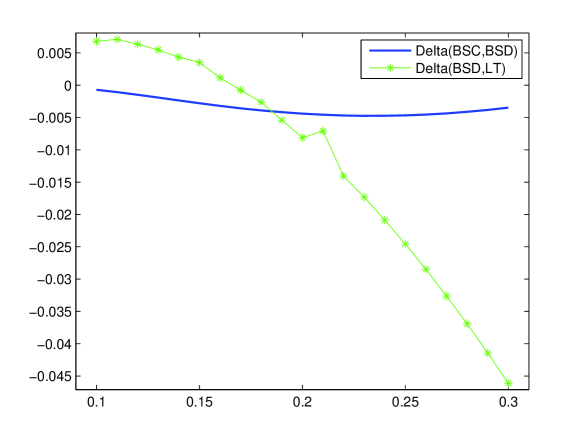
Figure 1: Comparison between EPE changes for fixed risk-free rates. $\Delta(BSD,BSC)$ vs $\Delta(BSD,LT)$ with $r=1\%$ and $K=3.75.$ The volatility parameter varies between $10\%$ and $30\%.$

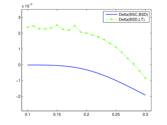
Figure 2: Comparison between EPE changes for fixed risk-free rates. $\Delta(BSD,BSC)$ vs $\Delta(BSD,LT)$ with $r=1\%$ and $K=4.78$ The volatility parameter varies between $10\%$ and $30\%.$

4.4 Some remarks about computational complexity

Once a new methodology or algorithm has been proposed, one would like to picture a general analysis of the computation complexity of the new method compared to its more traditional competitors; similarly for the accuracy and convergence rate. In the simplest and naive case, one has just one parameter, let it be N, e.g., the number of simulations, the number of deals in the portfolio, the number of time steps, etc., and the computational complexity could be stylized by a single “order” such as $O\left(N\right),\>O\left(N^{2}\right)$ and so on.

Despite this elegant theoretical approach, concrete applications are characterised by extra difficulties as, e.g.: (1) the proposal, or the set of competitors, could depend on some different parameters, and $N$ could not be a proper summary of the technique set up; (2) for each atomic algorithmic task, namely for any simulation of a loop of N simulations, the different competitors could contain calculations with very different levels of complexity and elapsed time, let them be $t_{1}$ and $t_{2}$. Hence it can happen that for small or medium values of the parameter N the actual computational time of the two algorithms do not match the asymptotic order ranking, e.g., it could be that $t_{1}\cdot N>t_{2}\cdot N^{3/2}.$ (3) finally, the observed computational times depend on many implementation details: the numerical integration method, bounded or not bounded integration, efficiency of the libraries embedded in the exploited programming languages.

Coming back to the above tables of execution times for BSD, BSC and LT, also focusing on the evaluation of the EE and EPE values, loops behave similarly with cross-method in increasing the number of calculations, and we observe that the BSC involves a time integration of the rather complicated BS formula, while the BSD has a complexity given by the $BS\cdot t_{n},$, the second term being the number of fixing times, and eventually the LT has a complexity given by time-space integration of a quite simple function which is the payoff itself.

Moreover, we optimized the latter by bounding both the inf and the sup of the space integral. Therefore, even without an exhaustive comparison, also considering different techniques implementations, we can conclude that the LT proposal allows for a good Accuracy versus Effort trade-off. We also underline that extensions to other market parameters, clauses and payoffs are needed.

5 Conclusions and Further Research

We have addressed the issue of the CCR assessment for the so-called accumulator derivatives, within the Black-Scholes  financial framework with one risky asset. Since the corresponding payoff depends on the time spent by a geometric Brownian Motionnear a given value, we have exploited the notion of BLT which turns to play a crucial role in the derivative pricing step for CCR evaluation.

However, it is possible to involve BLT also in the risk factors simulation step: roughly speaking, for each time bucket $t_{k},$ we could employ BLT to build up the grid $(t_{k},S_{t_{k},n})$ and the corresponding probabilities, and evaluate the $k$-th Expected Exposure $EE_{k}$ as the sum of weighted probability masses. We have proposed an original approach founded on the possibility of expressing the BLT in terms of its probability density. The associated implementation with regard to EPE evaluation leads to numerical results that significantly improve those obtained by standard procedures à la Black-Scholes. A smaller execution time and a better EE appraisal accuracy, makes our method a competitive tool, suggesting to extend the local time approach to more general derivatives, such as barrier options or Asian options. Next step consists in comparing our results with those derived in [18, 19].

Moreover, we also plan to use the results presented in [46], namely a generalization of the well-known Lévy’s Arc-sine Law, see also [36], which provides the distribution of the occupation time given in eq.  (12). In fact, we intend to use the related Takacs formula as an alternative expression for the probability density stated in  (4.2) which has been extensively used in this paper.

Finally, we are aware that the one-dimensional case turns out to be unrealistic, though relatively easy to implement, albeit to work in the $1$-dimension framework is a very acceptable proxy for derivatives of banks with corporate customers, i.e. small and medium size enterprises; in these cases the $i$-th customer has a very small number of deals, with main dependence on a single risk factor, e.g. the EUR interest rate curve. After all, a large number of risk factors entails a very hard estimation of correlations.

To overcome such drawbacks, financial institutions resort to some heuristic and easy-to-extend methods. For example, in the $2$-dimensional case it is common practice to consider $\left\langle\mathrm{d}W_{t}^{(1)},\mathrm{d}W_{t}^{(2)}\right\rangle=0$ between the asset classes, e.g. interest rate, forex or equity, and $\left\langle\mathrm{d}W_{t}^{(1)},\mathrm{d}W_{t}^{(2)}\right\rangle=\mathrm{d}t$ within the asset class. Such a procedure could be easily extended to the $N$-dimensional case, with $N>>1.$ This is clearly a complicated issue. From a theoretical point of view, the literature provides contributions related to the study of multidimensional BLT, see e.g. [11] and references therein.

References

- [1] Antonov A., Issakov S. and Mechkov S. (2015) Backward induction for future values, Numerix Research paper.
- [2] Banca d’Italia (2006) Circolare n. 263 - Nuove disposizioni di vigilanza prudenziale per le banche.
- [3] Banque de France (2007) Arrêté du 20 février 2007 relatif aux exigences de fonds propres applicables aux établissements de crédit et aux entreprises d’investissement.
- [4] Basel Committee on Banking Supervision (2006) Basel II: International Convergence of Capital Measurement and Capital Standards: A Revised Framework - Comprehensive Version, BCBS Paper 128.
- [5] Basel Committee on Banking Supervision (2011) Basel III: A global regulatory framework for more resilient banks and banking systems - revised version, BCBS Paper 189.
- [6] Bernis G. and Scotti S. (2017) Alternative to beta coefficients in the context of diffusions, Quant. Finance 2(17), 275–288.
- [7] Black F. and Scholes M. (1973) The pricing of options and corporate liabilities, Journal of political economy 3(81).
- [8] Bonollo M., Di Persio L., Oliva I. and Semmoloni A. (2015) A Quantization Approach to the Counterparty Credit Exposure Estimation, Available at SSRN: http://ssrn.com/abstract=2574384.
- [9] Borodin A.N. and Salminen P. (2002) Handbook of Brownian Motion: Facts and Formulae Birkhauser Verlag GmbH – Operator Theory, Advances and Applications.
- [10] Brigo D., Morini M. and Pallavicini A. (2013) Counterparty Credit Risk, Collateral and Funding: With Pricing Cases For All Asset Classes Wiley, Chichester.
- [11] Brydges D., Van Der Hofstad R. and Konig W. (2007) Joint density for the local times of continuous-time Markov chains, Ann. Prob. 4(35) 1307–1332.
- [12] Callegaro G., Fiorin L. and Grasselli M. (2015) Quantized calibration in local volatility, Risk (Cutting hedge: Derivatives pricing) April 56–67.
- [13] Callegaro,G., Fiorin L. and Grasselli M. (2017) Pricing via quantization in stochastic volatility models, Quant. Finance forthcoming.
- [14] Callegaro G. and Sagna A. (2013) An application to credit risk of a hybrid Monte Carlo-Optimal quantization method, J. Comput. Financ. 4(16) 123–156.
- [15] Carr P.P. and Jarrow R.A. (1990) The Stop-Loss Start-Gain Paradox and Option Valuation: A New Decomposition into Intrinsic and Time Value, Review of Financial Studies 3(3) 469–492.
- [16] Castagna A. (2013) Fast Computing in the CCR and CVA measurement, IASON Working paper.
- [17] Chevalier E., Ly Vath V. and Scotti S. (2013) An optimal dividend and investment control problem under debt constraints, SIAM J. Financ. Math. 4 297–326.
- [18] Cordoni F. and Di Persio L. (2014) Backward stochastic differential equations approach to hedging, option pricing and insurance problems, Int. j. stoch. anal., Vol. 2014.
- [19] Cordoni F. and Di Persio L. (2016) A bsde with delayed generator approach to pricing under counterparty risk and collateralization, Int. j. stoch. anal., Vol. 2016.
- [20] Di Persio L., Pellegrini G. and Bonollo M. (2015) Polynomial chaos expansion approach to interest rate models, J. Probab. Stat. (Online), Vol. 2015.
- [21] Di Persio L. and Perin I. (2015) An Ambit Stochastic Approach to Pricing Electricity Forward Contracts: The Case of the German Energy Market, Journal of Probability and Statistics, Vol. 2015.
- [22] Dellacherie C. and Meyer P.-A. (1979) Probabilities and Potential, Elsevier.
- [23] Doney R.A. and Yor M. (1998) On a Formula Of Takacs For Brownian Motion With Drift Journal of Applied Probability, 35 272–280.
- [24] Fujita T., Petit F. and Yor M. (2004) On the local time of the Brownian motion, Journal of Applied Probability 41(1) 1–18.
- [25] Fusai G. and Tagliani A. (2000) Pricing of occupation time derivatives: continuous and discrete monitoring, Journal Of Computational Finance, 5(1) 1–37.
- [26] Glasserman P. (2012) Risk Horizon and Rebalancing Horizon in Portfolio Risk Measurement Mathematical Finance 22(2) 215–249.
- [27] Gordy M.B. (2003) A risk-factor model foundation for rating-based bank capital rules, Journal of Financial Intermediation 12(3) 199–232.
- [28] Haug E.G. (1998) The Complete Guide to Option Pricing Formulas, McGraw-Hill Professional Publishing.
- [29] Heston S.L. (1993) A closed-form solution for options with stochastic volatility with applications to bond and currency options Review of Financial Studies 6 327–343.
- [30] Hull J. and White A. (1990) Pricing interest-rate derivative securities The Review of Financial Studies 3(4) 573–92.
- [31] Hull J. (1999) Options, futures, and other derivatives, Pearson Education India.
- [32] Karatzas I.A. and Shreve S.E. (1991) Brownian motion and stochastic calculus, Review of Financial Studies, Springer London, Limited.
- [33] Lam K., Yu P.L.H. and Xin L. (2009) Accumulator Pricing, CIFEr ’09. IEEE Symposium.
- [34] Lelong J. (2016) Pricing American options using martingale bases, Available at https://hal.archives-ouvertes.fr/hal-01299819.
- [35] Lévy P. (1939) Sur un problème de M. Marcinkiewicz. C. R. Acad. Sci. Paris Sèr. I Math. 208 318–321; errata 208 776.
- [36] Lévy P. (1939) Sur certains processus stochastiques homogènes. Compositio Math. 7 283–339.
- [37] Lévy P. (1965) Processus stochastiques et mouvement brownien, Gauthier-Villars, Paris.
- [38] Liu Q. (2015) Calculation of Credit Valuation Adjustment Based on Least Square Monte Carlo Methods, Mathematical Problems in Engineering, Vol. 2015.
- [39] Mijatovic A. (2010) Local time and the pricing of time-dependent barrier options, Finance Stoch 14 13–48.
- [40] Moody’s Global Corporate Finance, Corporate Default and Recovery Rates, 1920-2008, Moody’s Investors Service (Feb. 2009).
- [41] Pagés G. and Wilbertz B. (2011) Gpgpus in computational finance: Massive-parallel computing for American style options. Prebublications Labotatoire de Probabilite, Paris VI-VII.
- [42] Pykhtin M. and Zhu S. (2006) Measuring Counterparty Credit Risk for Trading Products under Basel II, Bank of America Working Paper.
- [43] Pykhtin M. and Zhu S. (2007) A Guide to Modelling Counterparty Credit Risk, GARP Association Review.
- [44] Saita F. (2007) Value at Risk and Bank Capital Management, Elsevier.
- [45] Sinkala W. and Nkalashe T.F. (2015) Lie Symmetry Analysis of a First-Order Feedback Model of Option Pricing, Advances in Mathematical Physics, Vol. 2015 (2015).
- [46] Takacs L. (1995) On the local time of the Brownian motion, Annals of Applied Probability 5(3) 741–756.
- [47] Vasicek O. (1977) An equilibrium characterization of the term structure Journal of Financial Economics, 5(2) 177–188.
- [48] Zhou Z. and Gao X. (2016) Numerical Methods for Pricing American Options with Time-Fractional PDE Models, Mathematical Problems in Engineering, Vol. 2016.